Sampling the conformational space of the catalytic subunit of human γ-secretase
- MRC Laboratory of Molecular Biology, United Kingdom
- Tsinghua University, China
Figures
Figure 1
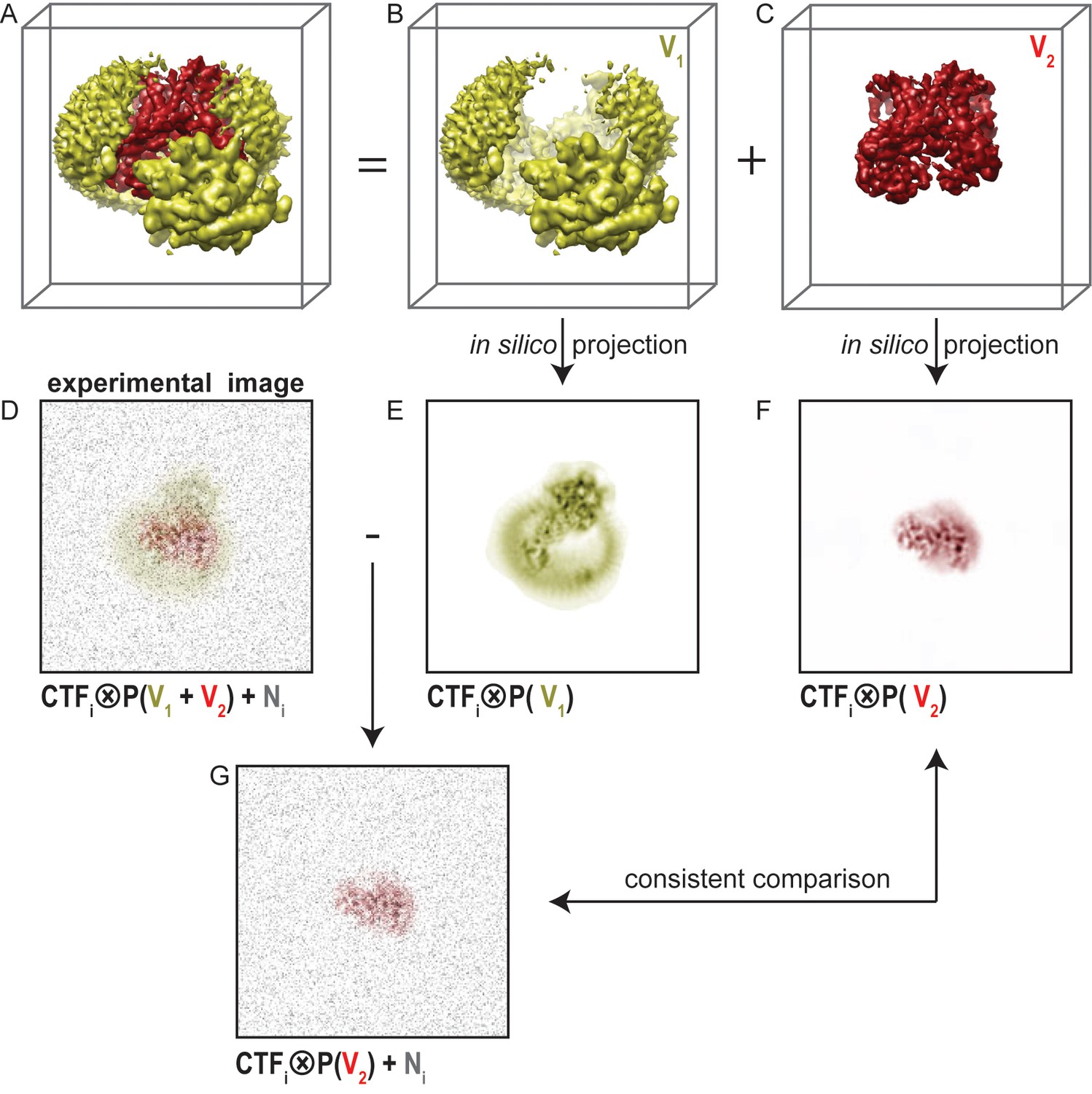
Masked classification with residual signal subtraction.
(A) A 3D model of a complex of interest. (B) The part of the complex one would like to ignore in masked classification (V1) is shown in yellow. (C) The part of the complex one would like to focus classification on (V2) is shown in red. (D) An experimental particle image is assumed to be a 2D projection of the entire complex in panel A that is affected by the contrast transfer function (CTF), and to which experimental noise (N, shown in grey) has been added. (E) A CTF-affected 2D projection of V1. (F) A CTF-affected 2D projection of V2. Previous approaches to masked classification in RELION (Amunts et al., 2014; Wong et al., 2014) compared experimental particles (panel D), with reference projections of only V2 (panel F). This results in inconsistent comparisons. (G) In the modified masked classification approach, one subtracts the CTF-affected 2D projection of V1 (panel E) from the experimental particle (panel D). This results in a modified experimental particle image that only contains experimental noise and the CTF-affected projection of V2, so that comparison with the reference projection in panel F becomes consistent.
Figure 2 with 4 supplements
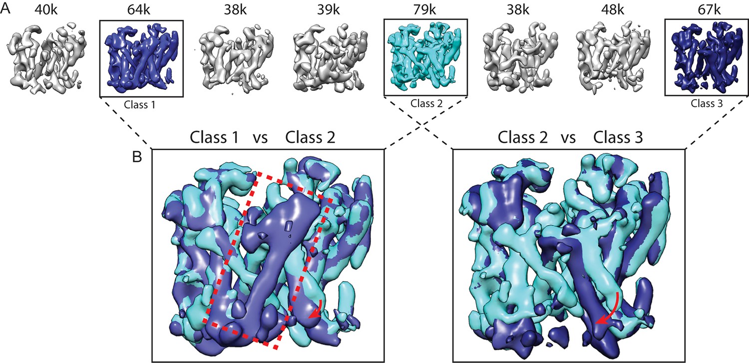
Masked classification with signal subtraction on PS1.
(A) From a masked 3D classification run on the PS1 subunit, the three largest classes (in cyan and blue, labeled class 1–3) showed good density. The five smallest classes (in grey) were ignored in further analyses as they showed suboptimal density. (B) Superposition of classes 1 and 2 and of classes 2 and 3 reveals the different orientations of TM6 in all three classes (indicated with red arrows), and the fact that TM2 (indicated with a red dashed box) is only ordered in class 1.
Figure 2—figure supplement 1

Cross-refinement of the masked classification results.
A 10Å low-pass filtered version of the map from class 3 (left) was refined against the particle subset identified for class 1. The resulting map (right) is undistinguishable from the original map from class 1, indicating that artifacts due to model bias did not play a role.
Figure 2—figure supplement 2
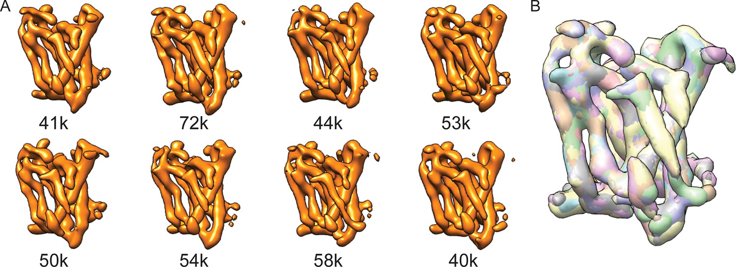
Masked classification on Aph-1.
(A) From a masked 3D classification run on the Aph-1 subunit with subtraction of the residual signal, all eight classes look very similar. (B) A superposition of all eight maps.
Figure 2—figure supplement 3
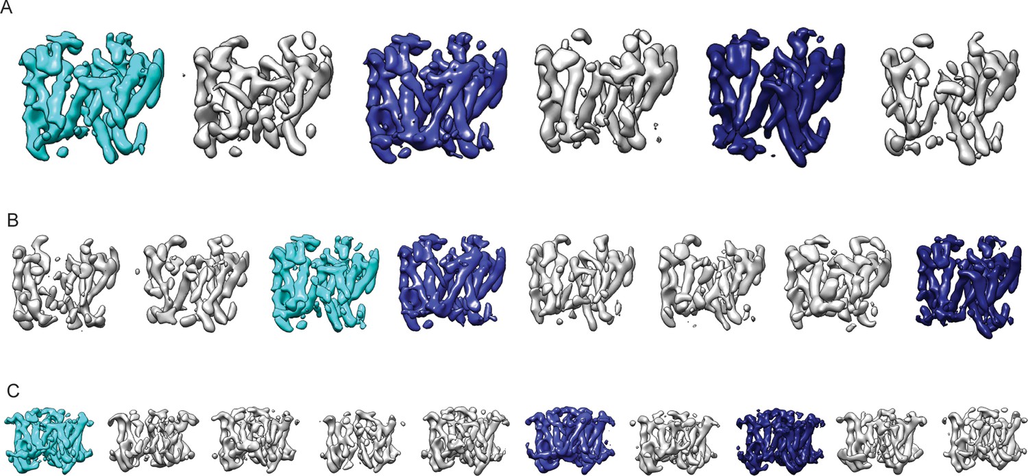
Reproducibility of masked classification on PS1.
Resulting maps from masked classifications on PS1 with subtraction of the residual signal using (A) six instead of eight classes; (B) a different random seed; and (C) ten classes and a slightly different mask from the run shown in Figure 2. The classes similar to the three largest classes shown in Figure 2 are highlighted in the same cyan and blue colors.
Figure 2—figure supplement 4
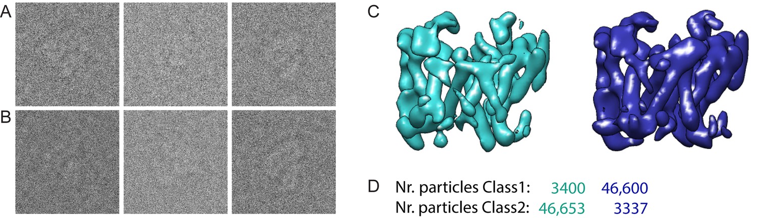
Masked classification with simulated data.
(A) Three examples of experimental particle images. (B) Three examples of simulated particle images. In total, 50,000 images of particles from Class 1 and 50,000 images of particles from Class 2 were simulated (also see Methods). (C) Resulting maps for a masked classification with signal subtraction on the catalytic subunit using two references. (D) Distribution of the simulated particles in the resulting classes: 93% of the particles were clustered correctly.
Figure 3 with 1 supplement
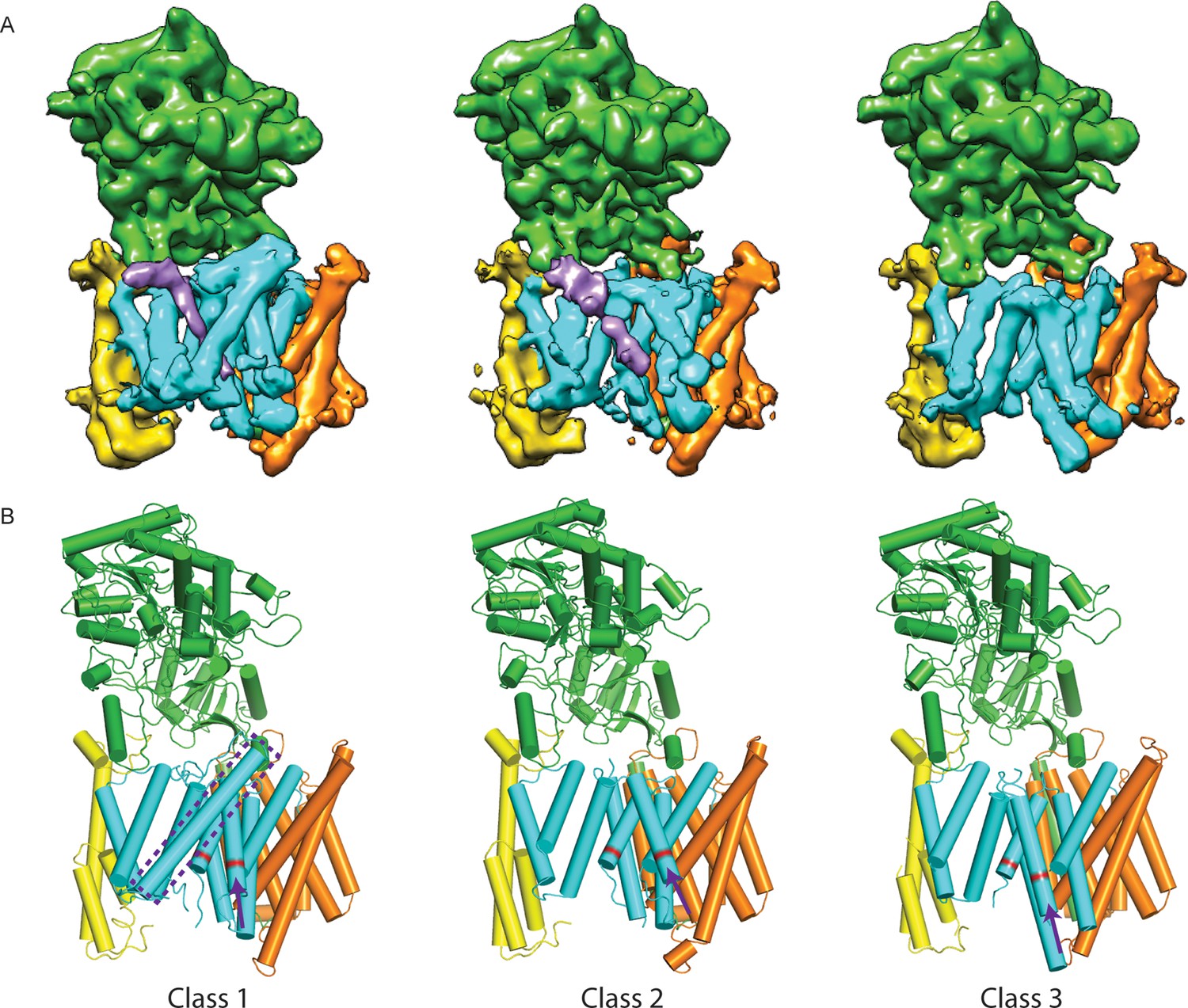
Three classes from the apo-state ensemble.
(A) The reconstructed density for the three classes. Nicastrin is shown in green, Aph-1 in orange, PS1 in cyan, and Pen-2 in yellow. α-Helical density that is unaccounted for by the γ-secretase model is shown in purple. The same color code is used throughout this paper. (B) Schematic representation of the γ-secretase atomic models. TMs of PS1 are numbered. The active site aspartates are shown in red. The purple dashed box highlights TM2 of PS1, which is only ordered in class 1. The purple arrows indicate the orientation of TM6, which is different in each class.
Figure 3—figure supplement 1
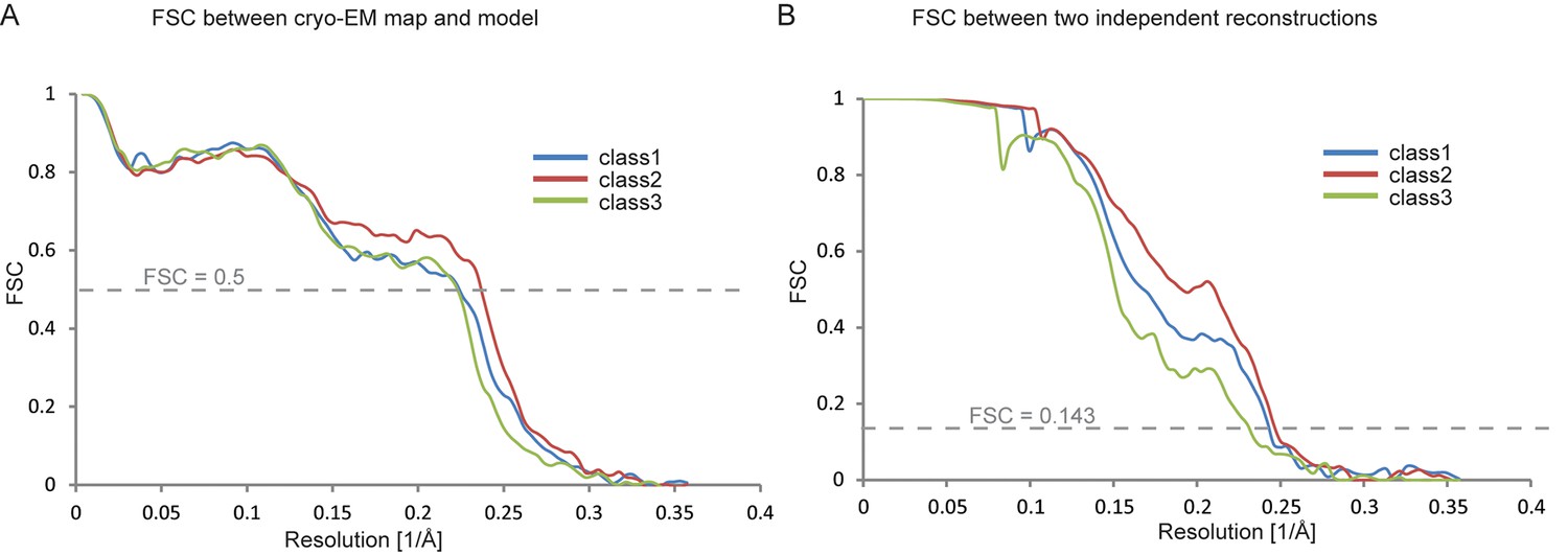
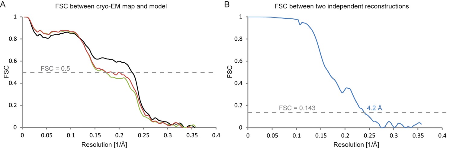
Fourier shell correlations for the three apo-state classes.
(A) FSC between the refined atomic models and the maps. (B) FSC between reconstructions from independently refined halves of the data sets.
Figure 4 with 1 supplement

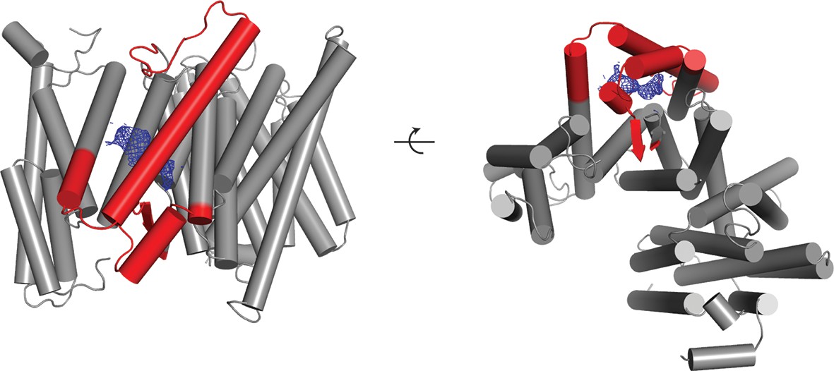
Helical density in class 1 of the apo-state ensemble.
(A–C) Three different views of the map and the atomic model are shown. The kinked α-helix that is unaccounted for by the γ-secretase model is shown in purple. PS1 residues that interact with this helix are labeled.
Figure 4—figure supplement 1

Mass spectrometry and Western blot analyses.
(A) The lower part of a Coomassie blue-stained SDS-PAGE gel of the γ-secretase sample that was also used for cryo-EM imaging was cut out and submitted for mass spectrometric analysis. Besides known γ-secretase components (bold text), several proteins with a single predicted transmembrane helix were also identified. (B) Western blot analyses confirmed the presence of at least three of the identified proteins in the sample. Arrowheads indicate their expected molecular weights.
Figure 5 with 4 supplements
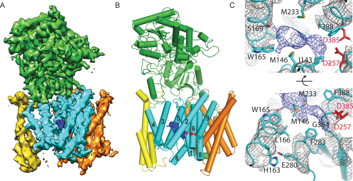
Cryo-EM structure of γ-secretase in complex with DAPT.
(A) The reconstructed density for the entire complex. Density attributed to DAPT is shown in blue. (B) Schematic representation of the atomic model. TMs of PS1 are numbered. (C) Two approximately orthogonal close-ups of the DAPT-binding site. Residues that interact with DAPT, as well as His163 and Glu280 are labeled.
Figure 5—figure supplement 1
Fourier shell correlations for the DAPT-bound structure.
(A) FSC curves of the refined atomic model versus the map it was refined against (in black); of a model refined in the first of the two independently refined half-maps versus that same map (in red); and of a model refined in the first of the two independent half-maps versus the second half-map (in green). (B) FSC between the two independently refined half-maps.
Figure 5—figure supplement 2

Masked classification with signal subtraction on the DAPT-bound data.
Using either masks around the PS1 subunit (top row) or the entire transmembrane domain (bottom row), masked classification with signal subtraction revealed only a single majority class (pink) that showed good density for the transmembrane helices (corresponding to 23% and 26% of the particles, respectively). In these maps, no helical-like density was observed in the cavity between TM2, TM3 and TM5 of PS1
Figure 5—figure supplement 3
Newly ordered elements in the DAPT-bound structure.
Two orthogonal views of a cartoon representation of the transmembrane domain of the DAPT-bound structure are shown. Those parts of the atomic model that were built in this structure but were disordered in the high-resolution consensus structure of the apo-state are shown in red. The density attributed to the DAPT molecule is shown in blue.
Figure 5—figure supplement 4

Similarity between the DAPT-bound structure of PS1 and class 1.
Two orthogonal views of an overlay of the DAPT-bound PS1 structure (in cyan) and class 1 of the apo-state ensemble (in grey) are shown. The catalytic aspartates in the DAPT-bound structure are shown in red.
Figure 6 with 1 supplement
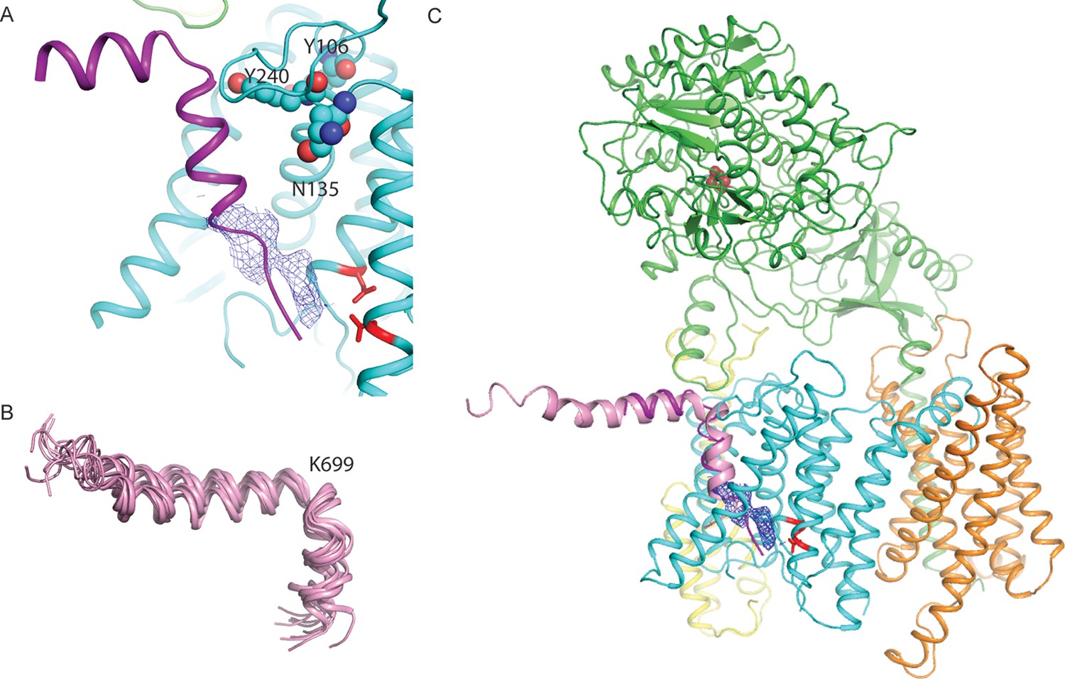
A hypothesis for substrate binding.
(A) A superposition of the kinked α-helix from class 1 and the DAPT-density and atomic model for PS1 from the DAPT-bound structure. The lower end of the kinked helix and the DAPT density overlap. The recently identified residues that interact with a phenylimidazole-like γ-secretase modulator are shown with spheres. (B) Ensemble of NMR-models for an Aβ42 peptide in an aqueous solution of fluorinated alcohols. (C) Hypothetical model for how APP (one of the NMR models is shown in pink) binds to γ-secretase.
Figure 6—figure supplement 1
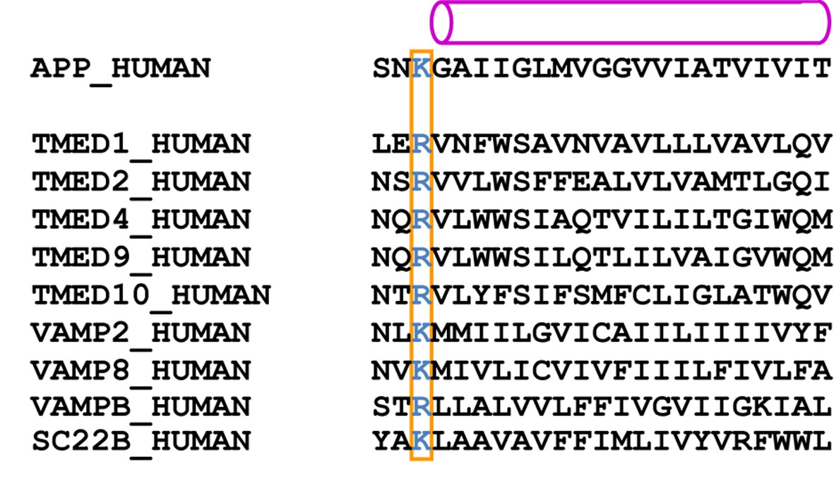
Predicted transmembrane regions.
APP and proteins that were identified by mass spectrometry to be present in the cryo-EM sample contain a large, positively charged residue (boxed) next to the N-terminus of their predicted transmembrane helix (indicated with a purple cylinder). TMP21 is the product of the TMED10 gene; P24a is the product of the TMED2 gene. The products of the TMED1, TMED4, TMED9, VAMP2 and VAMPB genes were observed after additional mass-spectrometric analysis of specific gel bands.
Videos
Video 1
A morph between the atomic models from class 1 and 2 of the apo-state ensemble.
https://doi.org/10.7554/eLife.11182.012
Video 2
A morph between the atomic models from class 2 and 3 of the apo-state ensemble.
https://doi.org/10.7554/eLife.11182.013Tables
Table 1
Refinement and model statistics
| Class1 | Class2 | Class3 | DAPT | |
|---|---|---|---|---|
| Data collection | ||||
| Particles | 63,873 | 79,263 | 66,720 | 51,366 |
| Pixel size (Å) | 1.4 | 1.4 | 1.4 | 1.4 |
| Defocus range (μm) | 0.7–3.2 | 0.7–3.2 | 0.7–3.2 | 0.6–2.8 |
| Voltage (kV) | 300 | 300 | 300 | 300 |
| Electron dose (e-/Å−2) | 40 | 40 | 40 | 40 |
| Map features | ||||
| Density TM2 | + | - | - | + |
| Cα-Cα distance D257– D385 (Å) | 9.5 | 12.7 | 9.1 | 8.0 |
| Conformation Pen-2 | in | in | out | in |
| α-helical density | + | + | - | - |
| Model composition | ||||
| Non-hydrogen atoms | 10,443 | 9,922 | 9,916 | 10,543 |
| Protein residues | 1,315 | 1,245 | 1,247 | 1,329 |
| Refinement | ||||
| Resolution (Å) | 4.1 | 4.0 | 4.3 | 4.2 |
| Map sharpening B-factor (Å2) | −100 | −100 | −130 | −130 |
| Fourier Shell Correlation | 0.8236 | 0.8818 | 0.8050 | 0.8602 |
| Rfactor | 0.2917 | 0.3028 | 0.2816 | 0.3426 |
| Rms deviations | ||||
| Bonds (Å) | 0.0112 | 0.0095 | 0.0120 | 0.0093 |
| Angles (°) | 1.7352 | 1.6083 | 1.7922 | 1.6186 |
| Model geometry | ||||
| Molprobity score | 3.17 | 2.89 | 3.16 | 3.22 |
| Clashscore (all atoms) | 17.35 | 9.31 | 13.26 | 18.15 |
| Good rotamers (%) | 89.6 | 90.9 | 86.6 | 88.9 |
| Ramachandran plot | ||||
| Favored (%) | 85.1 | 84.4 | 84.2 | 84.3 |
| Allowed (%) | 10.9 | 12.3 | 11.5 | 11.8 |
| Outliers (%) | 4.0 | 3.3 | 4.3 | 3.9 |
Download links
A two-part list of links to download the article, or parts of the article, in various formats.
Downloads (link to download the article as PDF)
Open citations (links to open the citations from this article in various online reference manager services)
Cite this article (links to download the citations from this article in formats compatible with various reference manager tools)
Sampling the conformational space of the catalytic subunit of human γ-secretase
eLife 4:e11182.
https://doi.org/10.7554/eLife.11182


