A new view of transcriptome complexity and regulation through the lens of local splicing variations
- University of Pennsylvania, United States
Figures
Figure 1
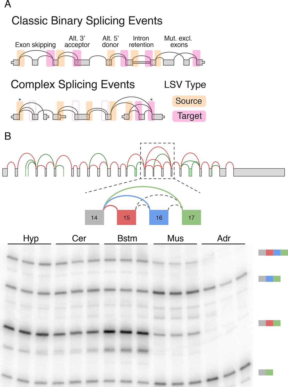
LSV formulation and prevalence.
(A) LSVs can be represented as splice graph splits from a single source exon (yellow) or into a single target exon (pink). LSV formulation captures previously defined, 'classical', binary alternative splicing cases (top) as well as other variations (bottom). An asterisk denotes complex variations involving more than two alternative junctions; dash line denotes redundant LSVs that are a subset of other LSVs (see Materials and methods). (B) Example of a complex LSV in the Camk2g gene. The gene’s splice graph (top) includes known splice junctions from annotated transcripts (red) and novel junctions (green) detected from RNA-Seq data. The splice graph includes a complex LSV involving exons 14–17 (middle). RT-PCR validation of the LSV in brainstem, cerebellum, hypothalamus, muscle, and adrenal is shown at the bottom. Several isoforms are preferentially included in brain and muscle.
Figure 2 with 2 supplements
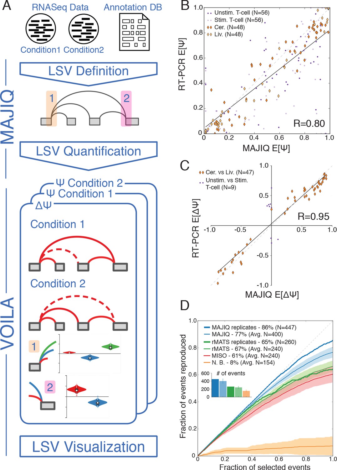
LSV analysis using MAJIQ.
(A) MAJIQ’s analysis pipeline. RNA-Seq reads are combined with an annotated transcriptome to create splice graphs and detect LSVs for each gene, then LSVs are quantified and compared between conditions. The visual output (VOILA) lists LSVs with violin plots representing estimates of percent inclusion index (PSI, Ψ) or changes in inclusion (dPSI, ΔΨ). Two cases are illustrated, for a single source three way LSV (orange), and a single target two way LSV (pink). (B) Correspondence between E[Ψ] by MAJIQ and Ψ by RT-PCR. R is the correlation coefficient. Colors and shapes represent different experimental conditions: mouse cerebellum and liver (dark and light orange diamonds, respectively); human unstimulated and stimulated T-Cells (dark and light purple dots, respectively). Total n = 208. (C) Correspondence between E[ΔΨ] by MAJIQ and ΔΨ by RT-PCR, where |ΔΨRT|>0.2. R is the correlation coefficient. Changes in inclusion were measured between liver and cerebellum mouse tissues (diamonds, n = 45); stimulated and unstimulated T-Cells (dots, n = 9). (D) Reproducibility ratio (RR) of high confidence differentially included LSVs, i.e. LSVs for which P(|ΔΨ|> 0.2) > 0.95), when comparing RNA-Seq from two conditions. A differentially included LSV is considered replicated if it maintains a rank at least as high as N in biological replicates, where N is the set size. LSVs are ranked by E[ΔΨ] and filtered for overlap. Twelve replicate pairs from Keane et al. (2011) were used to compute the histogram’s std (light blue). Other lines show MAJIQ’s RR with replicates (thick blue), RR for AS events detected by rMATS w/wo replicates (light and dark green), MISO (red), and RR for LSVs using Naïve Bootstrapping (orange). The inset bar chart shows the number of LSVs or AS events (N) derived by each method and used in the RR plots (see Materials and methods for more details).
Figure 2—figure supplement 1
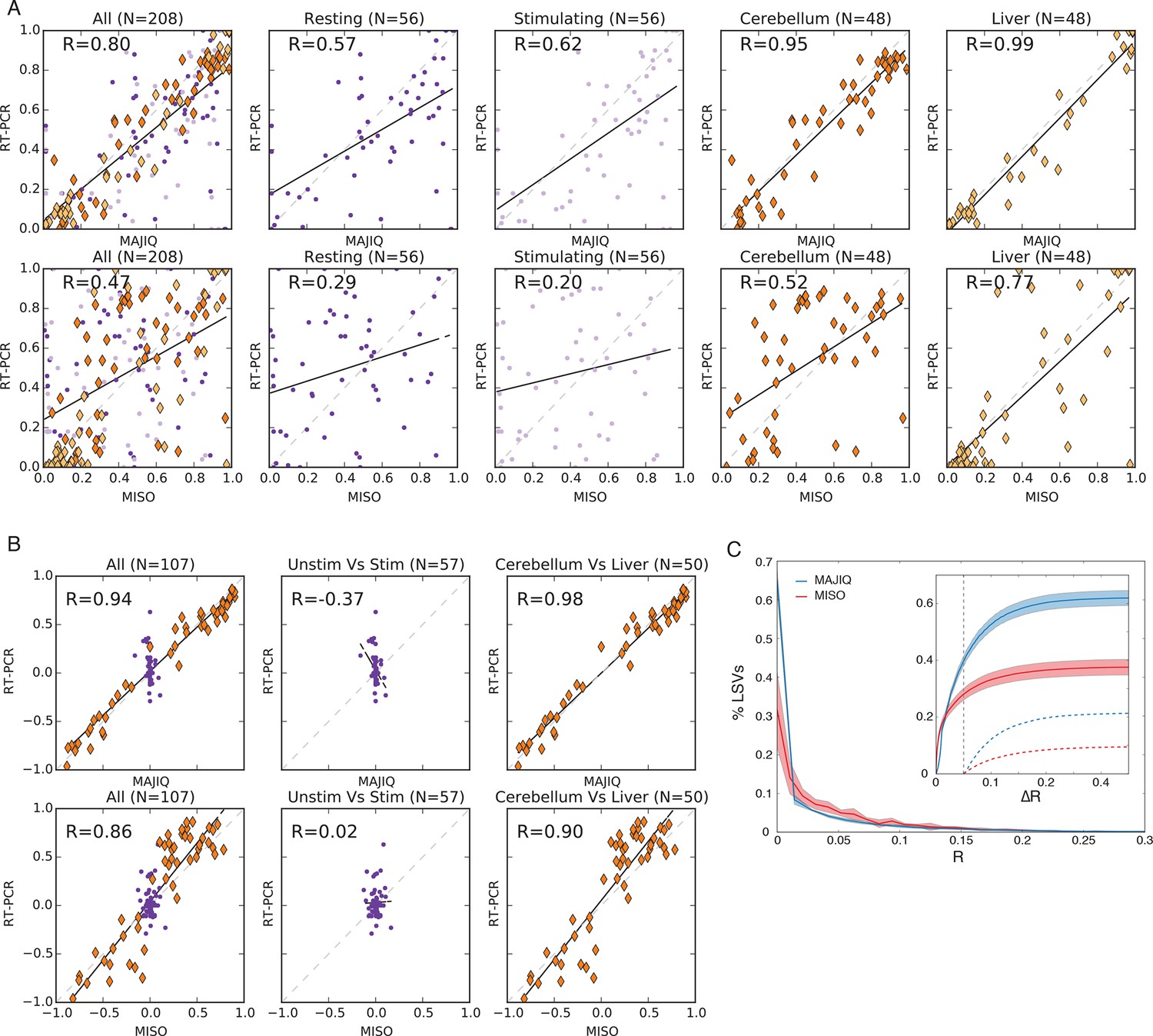
Quantifying PSI and dPSI accuracy.
(A) Correspondence between E[Ψ] by MAJIQ (top) or MISO (bottom) and Ψ by RT-PCR across four different experimental conditions. (B) The same set of LSVs used to measure correspondence between E[ΔΨ] by MAJIQ (top) and MISO (bottom) and ΔΨ by RT-PCR. Changes in inclusion were measured between cerebellum and liver mouse tissues (diamonds, right panel, n = 50); stimulated and unstimulated T-Cells (dots, center panel, n = 57). Setting a threshold of ΔΨRT =20% for a significant change MAJIQ has no false positives and fewer false negatives compared to MISO. (C) Histogram of Ψ reproducibility, computed as the absolute difference between biological replicates of hippocampus and liver (R = E[Ψr1]-E[Ψr1] ). Overall, 81.2% of the junctions in quantifiable LSVs were reproducible within 5% (R(Ψ) < 5%. Average n = 8058. Twelve replicate pairs were used to compute the histogram’s std (light color). Inset graph: comparing MAJIQ and MISO reproducibility for paired junction (ΔR = RMISO - RMAJIQ). Plot shows the cumulative distribution over ΔR>0 (blue) and ΔR<0 (red) and over the subset with significant difference ( ΔR >0.05, dashed lines). Overall MAJIQ improved Ψ reproducibility for approximately two thirds of the LSVs (P(ΔR = RMISO- RMAJIQ)> 0 = 61.7%) and over two fold more showed a significant improvement (P(ΔR>0.05) = 21.2%), P(ΔR< -0.05) = 10.1%).
Figure 2—figure supplement 2
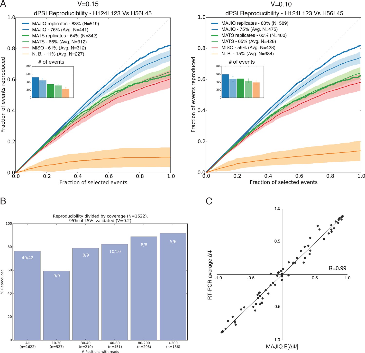
Quantifying differential splicing reproducibility.
(A) Effect of the threshold applied to the significance of splicing changes on the number of LSVs identified as changing (N) and the reproducibility ratio (RR). Both MAJIQ and rMATS estimate (P(ΔΨ) > α) > β) for an inclusion difference α with confidence level β. In the paper we used a strict β = 95% to control for false positives and a conservative α = 20% to call differentially spliced LSVs. Here, the results with a relaxed criteria of α = 15% (left) and α = 10% (right) are shown. The plots are otherwise identical to Figure 2D. (B) Breakup by coverage level (x-axis) of the high confidence differentially spliced LSVs depicted in Figure 2D. Y-axis denotes reproducibility ratio by RNA-Seq from biological replicates and the numbers at the top of each bar denote reproducibility by RT-PCR (|ΔΨRT|>0.2) of a randomly chosen subset of LSVs from that bin. The overall reproducibility is represented by the far left bin. (C) Correlation between MAJIQ E[ΔΨ] and average ΔΨ by RT-PCR among 3 biologic replicates for the most changing junction in validated complex LSVs examined in this paper between various pairs of tissues (n = 78). Of the junctions predicted to change between tissues (|E[ΔΨ]| > 20%), 55/56 validated (98.2%) by RT-PCR with an average |ΔΨ| > 20%.
Figure 3
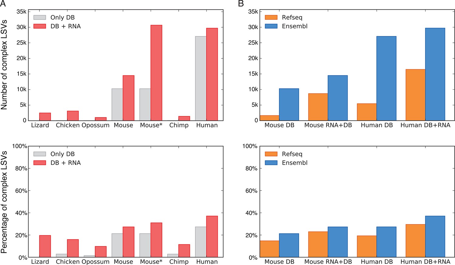
LSV prevalence across diverse metazoans.
(A) Number of LSVs (top) and fraction of complex LSVs (bottom) when using Ensembl annotated transcripts only (grey) or combining it with RNA-Seq from 5–6 similar tissues (red). Mouse* is the dataset from Zhang et al. (2014). (B) Number of LSVs (top) and fraction of complex LSVs (bottom) when using RefSeq (orange) and Ensembl (blue). The RNA-Seq dataset is the same as in (A).
Figure 4 with 1 supplement
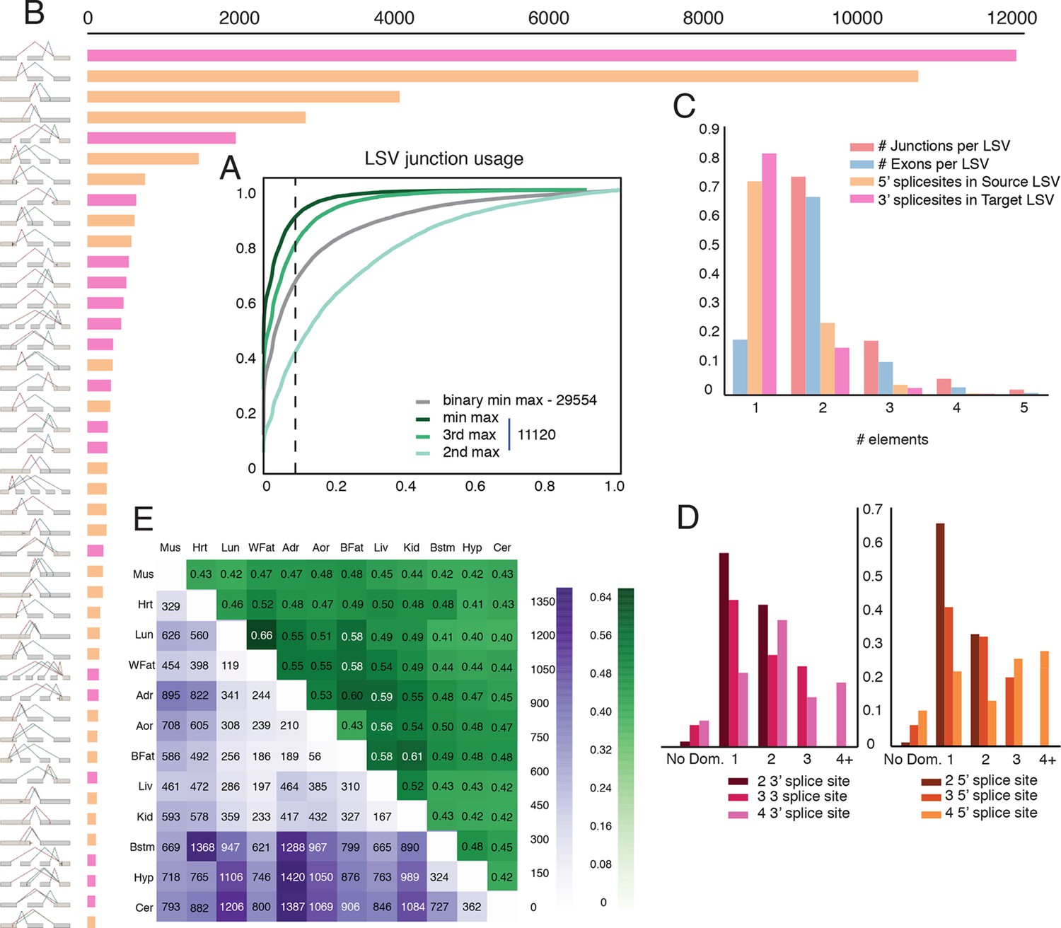
Genome wide view of exonic LSVs across twelve mouse tissues.
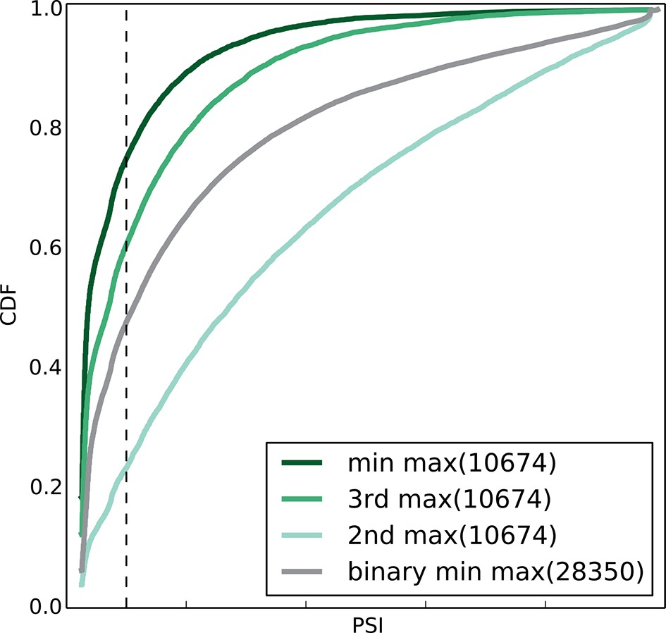
(A) Cumulative distribution (CDF) for maximal junction inclusion (PSI) across tissues. Plot includes the least used junction in binary LSV (grey), the second, third and least used junction in complex LSVs (light, medium, dark green). Dashed vertical line denotes 10% inclusion. (B) Histogram of the most common exonic LSV types. (C) Histogram of the number of exons, junctions, 3’ and 5’ splice sites in all identified LSV. (D) Histogram of which 3’ (left) or 5’ (right) splice site are found to be dominant across all tissues and all LSVs. X-axis denotes the order of the splice site. Dominance is defined as E[Ψ] > 0.6. Cases with no dominant junction are represented by the bars on the far left. (E) The fraction of complex LSVs (green, top right) from the total number (purple, bottom left) of differentially spliced LSVs (|E[ΔΨ]| >0.2) between pairs of tissues.
-
Figure 4—source data 1
dPSI values for all pairs of tissues.
- https://doi.org/10.7554/eLife.11752.009
Figure 4—figure supplement 1
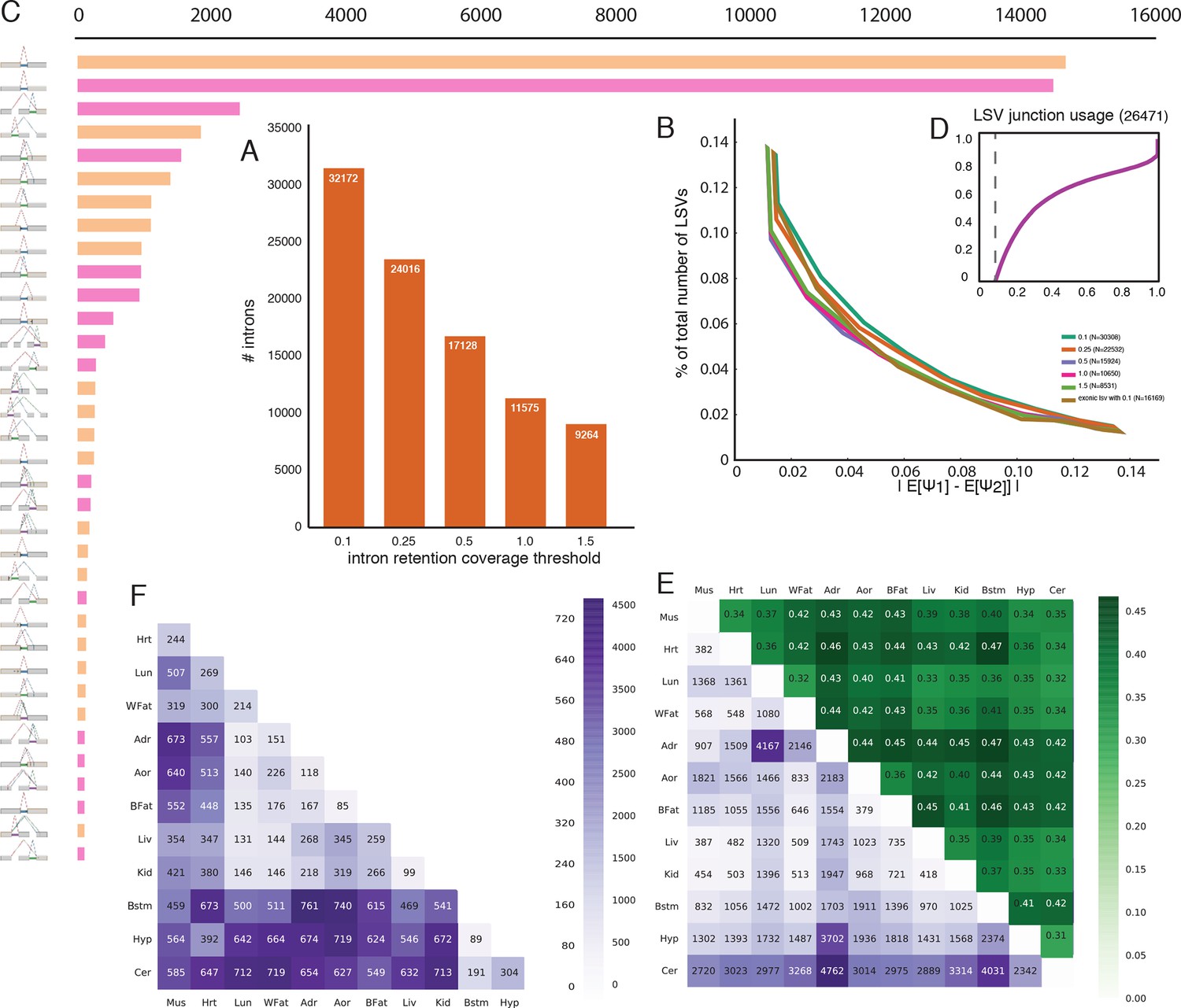
Intronic LSV detection and quantification.
(A) Effect of intronic average coverage on the number of detected introns in LSVs. (B) Histogram of mean Ψ reproducibility as in Figure 2—figure supplement 1C but for intronic LSV. Ψ Reproducibility is computed as the absolute difference between biological replicates (R = |E[Ψr1]-E[Ψr1]| ). Twelve replicate pairs were used to compute each histogram’s mean. The histograms’ std was too small to be plotted clearly. Colors correspond to different thresholds on average intronic coverage. Numbers in the legend represent average number of introns quantified in experiment pairs. Based on the tradeoff between reproducibility and overall detection shown in (A) subsequent evaluations and figures were executed using average intronic coverage threshold of 0.5. (C) Histogram of the most common intronic LSV types. Only non-redundant LSVs are included (See Materials and methods). (D) Cumulative distribution function for the fraction of the introns in intronic LSVs as a function of the minimal intronic Ψ observed across the twelve mouse tissues. Vertical dashed line corresponds to Ψ=10%. (E) Bottom left (purple): Each entry A(i,j) is the number of intron containing LSVs where the intron is differentially spliced between tissue i and tissue j. Upper right (green): Each entry A(i,j) is the fraction of complex LSVs from the LSVs listed in the matching bottom left rectangle entry A(j,i). Diagonal (red): Each entry A(i,i) is the total number of unique differentially spliced intron containing LSVs in tissue i compared to all other tissues where the intron is differentially spliced. (F) Bottom left (purple): Each entry A(i,j) is the number of intron containing LSVs where an exonic junction (and not the intron) is differentially spliced between tissue i and tissue j. Note that in this case the upper right (green) triangle that gives the fraction of complex LSVs from the LSVs listed in the matching bottom left rectangle is by definition 100% and is therefore not shown.
Figure 5 with 1 supplement
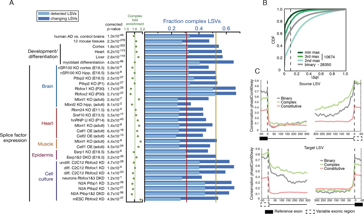
Meta analysis of complex LSVs.
(A) Fold enrichment (green dots) of complex LSVs calculated by comparing the fraction of complex LSVs among differentially spliced LSVs (dark blue bars) to their relative proportion (light blue bars) in 32 datasets. The corrected p-value column on the left measures significance of the fold enrichment (binomial test, Bonferroni corrected p-value) Medians are displayed for fold enrichment (green line, 1.63), fraction of complex LSVs among changing LSVs (orange line, 0.52), and fraction of complex LSVs among all detected LSVs (red line, 0.31). Human AD versus healthy brain data corresponds to the cohort from (Bai et al., 2013). See Figure 5—source data 1 for more information. (B) Empirical cumulative distribution function (CDF) of the maximal change of junction inclusion ( ΔΨ ) across all mouse datasets in Figure 5A. Only the LSVs detected in the twelve mouse tissues (Figure 4) are included. The plot includes junctions in binary LSVs (grey), and the second, third, and least changing junction in complex LSVs (light, medium, dark green). Dashed vertical line denotes ΔΨ of 10%. (C) Per nucleotide average conservation score (phastCons60 track) in regions proximal to single source (top) and single target (bottom) LSVs that were differentially spliced between any pair of tissues shown in Figure 4. The average is plotted for the subsets of complex (green) LSVs and binary (grey) LSVs as well as around a randomly selected set of constitutively spliced junctions (red, see Materials and methods for details).
-
Figure 5—source data 1
LSV enrichment meta analysis table.
- https://doi.org/10.7554/eLife.11752.012
Figure 5—figure supplement 1
Empirical cumulative distribution function (CDF) of the maximal junction inclusion (E[Ψ]) across all mouse datasets in Figure 5A.
Only the LSVs detected in the twelve mouse tissues (Figure 4) are included. This plot is equivalent to the ΔΨ plot in Figure 5B and includes junctions in binary LSVs (grey), as well as the second, third, and least included junction in complex LSVs (light, medium, dark green). Dashed vertical line denotes 10% inclusion.
Figure 6 with 2 supplements

Identification of a novel, brain-specific, PTC-introducing, developmentally-regulated exon in Ptbp1.
(A) Top: Splice graph representation of a complex target LSV containing a previously unannotated, PTC-introducing exon in Ptbp1 (exon 14, green). Stop signs indicate multiple conserved premature termination codons. Bottom: UCSC Genome Browser tracks of RNA-seq reads from adrenal (red) and cerebellum (blue), and conserved Rbfox binding sites ([U]GCAUG) found within the bounds of this LSV. (B) Top panel: RT-PCR validation of RNA from replicate cerebellar and adrenal tissues with isoforms illustrated on the left. Asterisk denotes a background band that migrates non-specifically. Bottom panel: E[Ψ] violin plots of MAJIQ quantification for the colored junctions in (A). Matching isoforms are indicated on the left. (C) Top: RNA-seq reads from mouse cortices (Yan et al., 2015). Developmental time points indicated on the right with exons colored as in (A). Bottom: Ψ violin plots for the PTC-introducing exon 14 across brain development. (D) Top panel: Top regulatory motifs predicted by AVISPA to influence the neuronal-specific splicing of exon 14. Stacked bars represent the normalized feature effect (NFE) for each motif. Colors indicate the contribution of the corresponding motif in the region indicated in the inset. (E) MAJIQ Ψ quantification of the LSV shown in (A), using RNA-seq from one month old wild type whole brain (left) and nestin-specific Rbfox1 KO littermates (right).
Figure 6—figure supplement 1
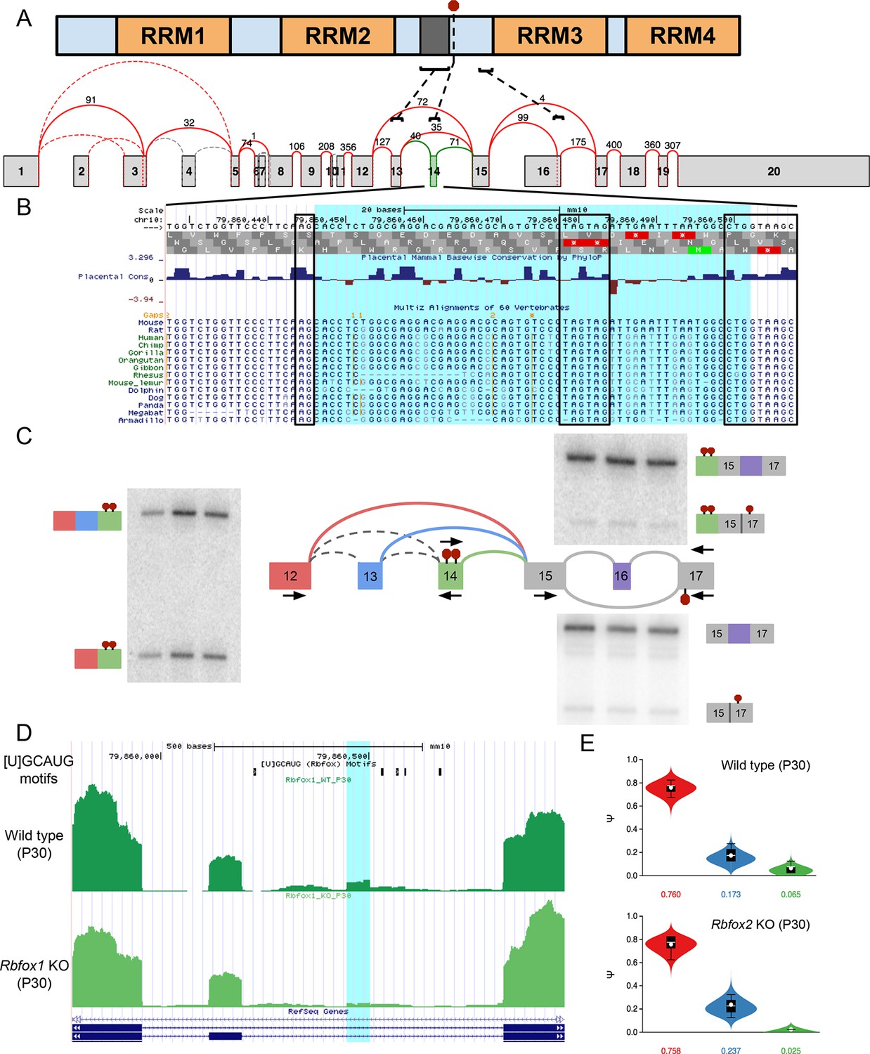
Novel exon and PTCs in Ptbp1 are conserved, independent from known PTC event, and regulated by Rbfox1 and 2.
(A) PTBP1 domain structure (top) and splice graph from cerebellum data (bottom) highlighting approximate locations of known alternatively spliced linker region (dark grey) encoded by exon 13 (exon 9 in the literature), the novel PTC introducing exon 14 (red stop sign in protein, green exon in splice graph), and the known PTC upon exclusion of exon 16 (exon 11 in the literature). (B) UCSC genome browser view with sequence alignment and placental mammalian conservation. Novel exon 14 is highlighted in blue and boxed regions correspond to conservation of 3’ and 5’ splice sites and the in frame PTCs. (C) Locations of additional primers with RT-PCR from replicate cerebellum RNA. (D) UCSC genome browser view showing conserved Rbfox binding sites ([U]GCAUG) and brain RNA-seq reads from wild type one month old mice (top) and Rbfox1 KO littermates (bottom) corresponding to experiments quantified in Figure 6E. Exon 14 location is highlighted in blue. (E) MAJIQ Ψ quantification of junctions as illustrated in (C) from one month old wild type mice (top) and Rbfox2 KO littermates (bottom).
Figure 6—figure supplement 2
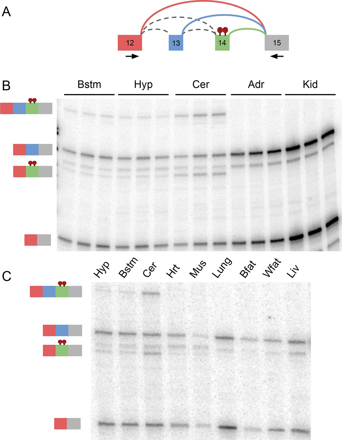
RT-PCR validation of complex Ptbp1 LSV across 11 mouse tissues.
(A) Representation of Ptbp1 target LSV analyzed with primers indicated by arrows. (B) RT-PCR from replicates across tissues indicated with isoforms indicated on the left. (C) Representative RT-PCR from tissues indicated with isoforms indicated on the left. [Bstm: brainstem; Hyp: hypothalamus; Cer: cerebellum; Adr: adrenal gland; Kid: kidney; Hrt: heart; Mus: muscle; Bfat: brown adipose; Wfat: white adipose; Liv: liver]
Figure 7 with 7 supplements
Camk2d LSV exhibits complex developmental dynamics and is misregulated in Alzheimer’s disease.
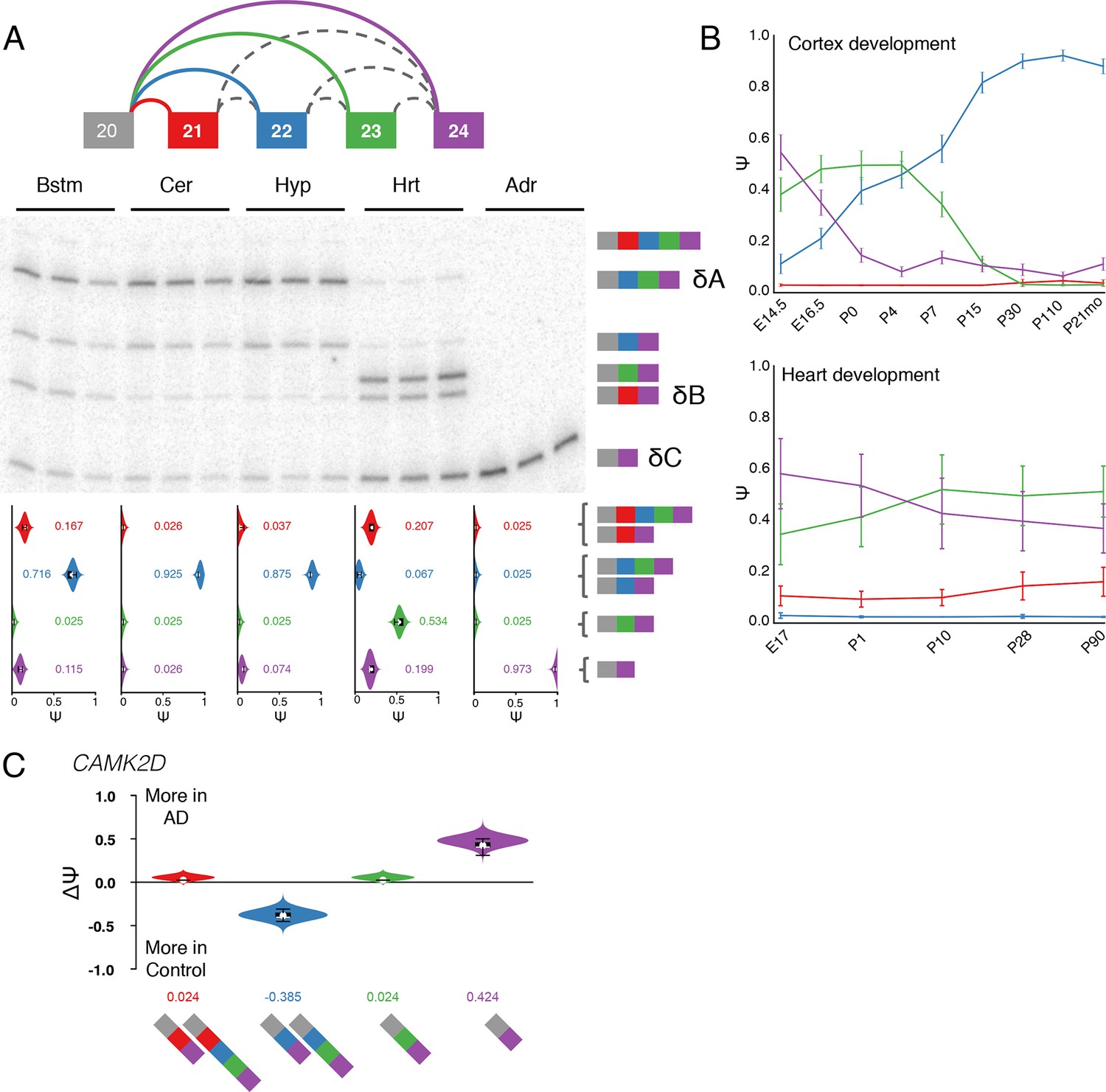
(A) Representation of complex source LSV in Camk2d with matching RT-PCR validation in five tissues (brainstem, cerebellum, hypothalamus, heart, and adrenal). Colored arcs represent the junctions quantified by MAJIQ for this LSV while dashed arcs correspond to junctions in the RNA-seq data that are not part of the quantified LSV. Violin plots on the bottom display Ψ quantifications (x-axis) for each of the colored junctions (y-axis) across the five tissues with appropriate isoforms from the gel on the right. Isoforms with known tissue-specific splicing patterns are labeled as in the literature (B) Line graphs of MAJIQ E[Ψ] quantification (y-axis) of junctions as in (A) across time points (x-axis) through cortex development (top) and heart development (bottom). Points represent mean Ψ and error bars represent one standard deviation in E[Ψ]. (C) ΔΨ quantification comparing changes between control and Alzheimer’s patient brains of the homologous junctions illustrated in (A).
Figure 7—figure supplement 1
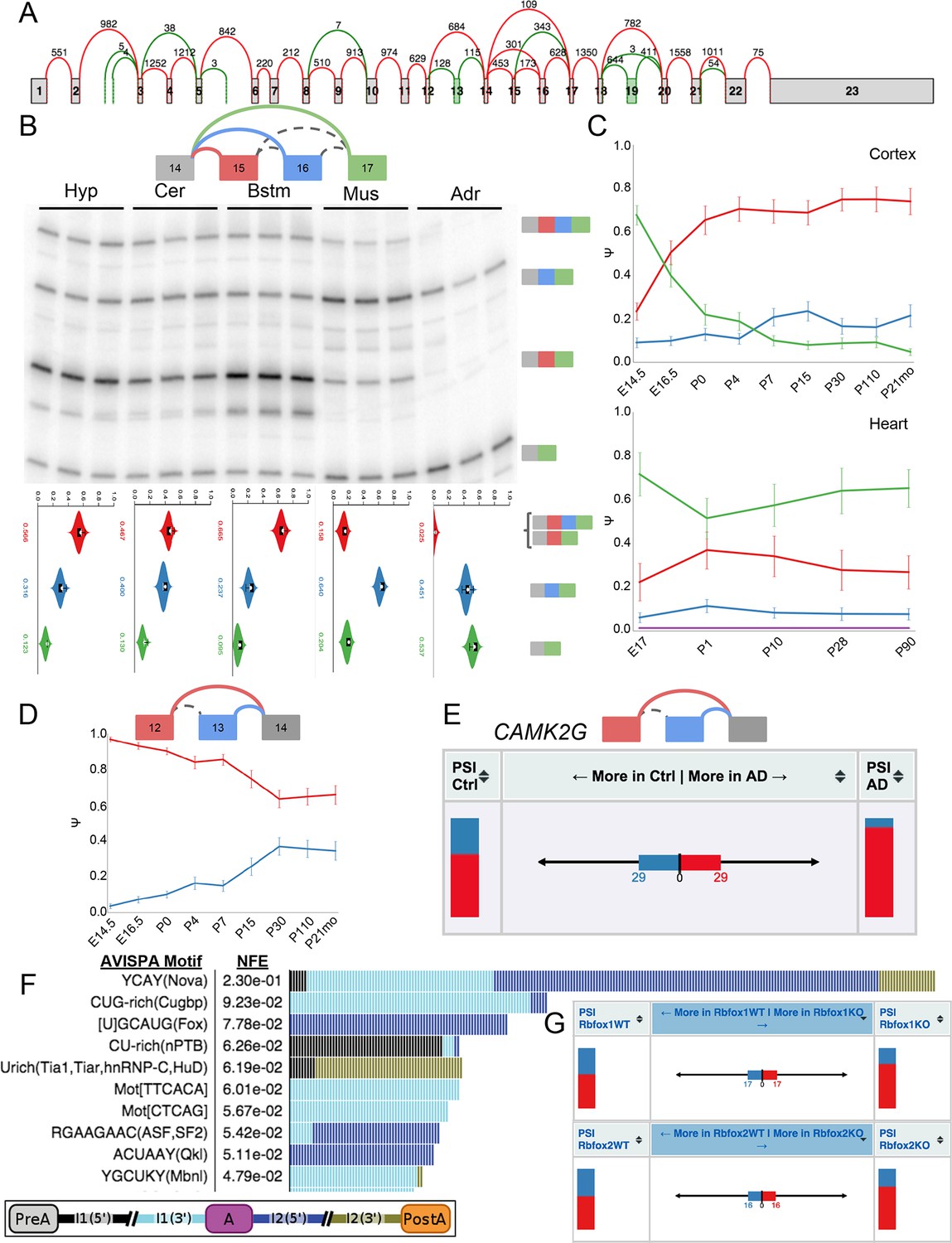
Complex and de novo LSVs in Camk2g are developmentally regulated and dysregulated in Alzheimer’s disease.
(A) Splice graph representation of Camk2g in the cerebellum. Green junctions and exons denote de novo detection from RNA-seq data. Numbers represent number of raw reads across the junction. (B) Representation of complex source LSV in Camk2g (top) with matching RT-PCR validation in five tissues (brainstem, cerebellum, hypothalamus, heart, and adrenal, middle). Colored arcs represent the junctions quantified by MAJIQ for this LSV while dashed arcs correspond to junctions in the RNA-seq data, but not directly quantified by the LSV. Violin plots on the bottom display E[Ψ] quantifications (x-axis) for each of the colored junctions (y-axis) across the five tissues with appropriate isoforms from the gel on the right. (C) Line graphs of MAJIQ Ψ quantification (y-axis) of junctions as in (B) across time points (x-axis) through cortex development (top) and heart development (bottom). Points represent mean Ψ and error bars represent one standard deviation. (D) Representation of de novo exon 13 detected in mouse (top) and MAJIQ Ψ across mouse cortex development, points represent mean Ψ and error bars represent one standard deviation (bottom). (E) VOILA ΔΨ visualization of LSV from (D) that is conserved in human showing E[Ψ] values (stacked bar chart, sides) and E[ΔΨ] (center) for each junction between control and Alzheimer’s disease brains. (F) Top regulatory motifs predicted by AVISPA to influence the CNS splicing patterns of exon 13. Stacked bars represent the normalized feature effect (NFE) for each motif as in (Barash et al., 2013). Colors indicate the contribution of the corresponding motif in the region indicated in the inset. (G) VOILA ΔΨ visualization LSV from (B) showing E[Ψ] values (stacked bar chart, sides) and E[ΔΨ] (center) between wild type and Rbfox1 (top) or Rbfox2 (bottom) KO mice.
Figure 7—figure supplement 2

LSV in Camk2a is developmentally regulated oppositely in the brain and heart.
(A) Splice graph representation of Camk2a across three tissues indicated. Dashed box indicates region containing cassette exon that inserts a consensus NLS. (B) MAJIQ E[ΔΨ] between cerebellum and muscle for inclusion (green) and exclusion (blue) isoforms. Red junction corresponds to an alternative 5’ss not highly used in any tissue. (C) Line graphs of MAJIQ Ψ quantification (y-axis) of junctions as in (B) across time points (x-axis) through cortex development (left) and heart development (right). Points represent mean Ψ and error bars represent one standard deviation.
Figure 7—figure supplement 3

Developmentally controlled, complex LSV in Camk2b is regulated by Ptbp2.
(A) VOILA thumbnail representation of complex target LSV in Camk2b detected from cortex development data including a alternative transcription start in exon 21 (green junction) that is not highly utilized and NAGNAG alternative 3’ splice sites of reference exon 22. (B) Line graphs of MAJIQ Ψ quantification (y-axis) of junctions as in (A) across time points (x-axis) through cortex development show known increase in exon 20 inclusion through development, coupled with a novel switch from proximal NAG 3’ss (red) to almost exclusive use of distal NAG 3’ss (orange) by adulthood. Points represent mean Ψ and error bars represent one standard deviation. (C) UCSC genome browser view of mapped reads from cortex of embryonic 16.5 mouse (top, purple) or postnatal 21-month mouse (bottom, blue). Dashed box highlights nucleotides corresponding to conserved NAGNAG alternative 3’ss that is developmentally regulated. (D) Top regulatory motifs predicted by AVISPA to influence the CNS splicing patterns of exon 20. Stacked bars represent the normalized feature effect (NFE) for each motif. Colors indicate the contribution of the corresponding motif in the region indicated in the inset. (E) Violin plots representing MAJIQ Ψ for wild type E18.5 mice (top) and Ptbp2 KO littermates (bottom) shows embryonic Ptbp2 represses adult specific inclusion of exon 20, as previously reported (Li et al., 2014), in addition to the switch in NAGNAG 3’ splice site use.
Figure 7—figure supplement 4
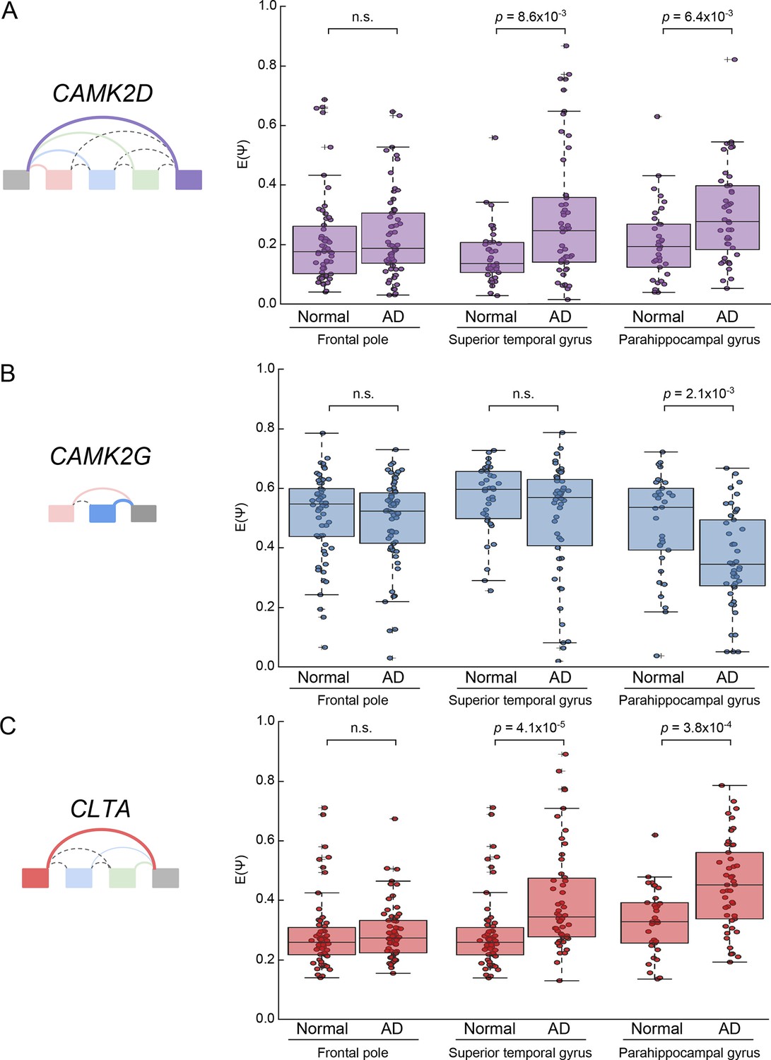
Analysis of CAMK2D, CAMK2D, and CLTA LSVs in an independent Alzheimer’s cohort.
(A) Boxplot showing distribution of E[Ψ] values and all E[Ψ] values (dots) for the most changing junction in the CAMK2D event examined in Figure 7 from a larger, independent cohort of normal and AD patients in the given brain sub regions. Two-tailed rank sum p-values are shown. (B) Same as (A) but for CAMK2G event examined in Figure 7—figure supplement 1. (C) Same as (A) but for CLTA event examined in Figure 7—figure supplement 6. Total samples analyzed for frontal pole normal and AD are 58 and 62; superior temporal gyrus normal and AD, 37 and 50; parahippocampal gyrus normal and AD, 33 and 45.
Figure 7—figure supplement 5
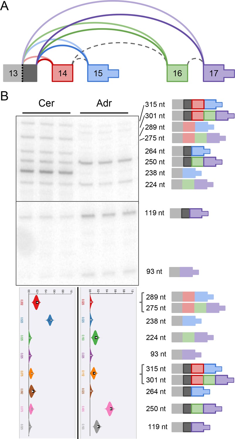
Complex alternative end of Alzheimer’s-associated Klc1.
(A) Splice graph representation of a complex alternative end LSV of Klc1. Dark grey represents a 26 nt alternative 5’ss of exon 13. (B) Top panel: RT-PCR validation with RNA from replicate cerebellar and adrenal tissues with isoforms illustrated on the left. Dark outlined isoforms are those that include the 26 nt alternative 5’ss of exon 13. Bottom panel: PSI violin plots of MAJIQ quantification of junctions as colored in (A).
Figure 7—figure supplement 6

Clta splicing is developmentally regulated and dysregulated in Alzheimer’s Disease.
(A) Splice graph for Clta and representation of target LSV. (B) Top panel: RT-PCR validation with RNA from replicate tissues with isoforms illustrated on the left. Bottom panel: PSI violin plots of MAJIQ quantification of junctions as colored in (A). (C) Line graphs of MAJIQ Ψ quantification (y-axis) of junctions as in (A) across time points (x-axis) through cortex development. Points represent mean Ψ and error bars represent one standard deviation. (D) ΔΨ quantification comparing changes between control and Alzheimer’s patient brains of the homologous junctions illustrated in (A).
Figure 7—figure supplement 7
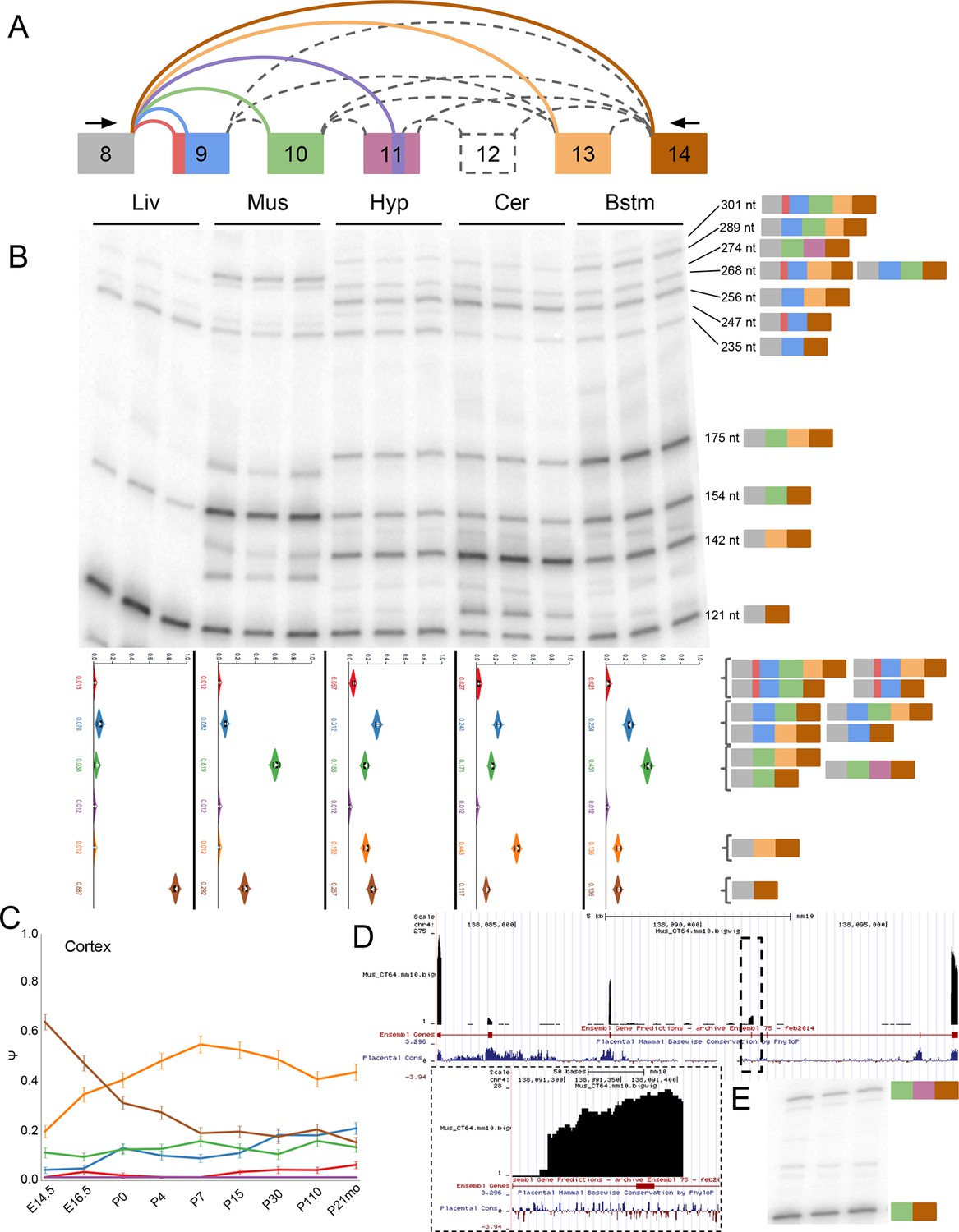
Eif4g3 splicing shows brain subregion-specificity and a novel exon in muscle.
(A) Representation of complex source LSV in Eif4g3. Red junction, red portion of exon 10 correspond to a novel alternative 3’ss detected in the brain. Purple junction, purple portion of exon 12, and dashed exon 13 correspond to Ensembl annotated tandem cassette exons with no support in any experiment. Larger, pink portion of exon 12 corresponds to 120 nt, unannotated exon that is included with exon 11 in muscle. (B) Top panel: RT-PCR validation with RNA from replicate tissues with isoforms and expected product sizes illustrated on the left. Bottom panel: PSI violin plots of MAJIQ quantification of junctions as colored in (A). (C) Line graphs of MAJIQ Ψ quantification (y-axis) of junctions as in (A) across time points (x-axis) through cortex development. Points represent mean Ψ and error bars represent one standard deviation. (D) UCSC genome browser view of the bounds of this LSV with mapped reads from representative muscle sample. Inset shows zoomed area of dashed lines corresponding to the location of the novel bounds of exon 11 . (E) RT-PCR from replicate muscle RNA using an additional primer set from exon 10 to 14.
Additional files
-
Supplementary file 1
Protein features enrichment analysis results.
- https://doi.org/10.7554/eLife.11752.025
-
Supplementary file 2
List of primers used for experimental validation.
- https://doi.org/10.7554/eLife.11752.026
Download links
A two-part list of links to download the article, or parts of the article, in various formats.
Downloads (link to download the article as PDF)
Open citations (links to open the citations from this article in various online reference manager services)
Cite this article (links to download the citations from this article in formats compatible with various reference manager tools)
A new view of transcriptome complexity and regulation through the lens of local splicing variations
eLife 5:e11752.
https://doi.org/10.7554/eLife.11752


