A stochastic neuronal model predicts random search behaviors at multiple spatial scales in C. elegans
Figures
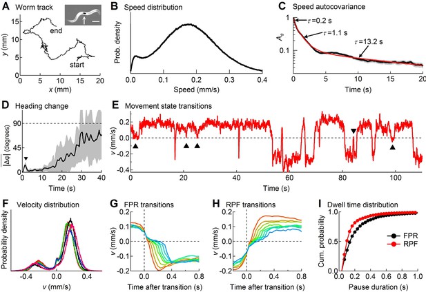
Descriptive statistics of wild type worm tracks.
(A) -coordinates of a worm during 10 min of foraging. Inset: Image of a worm showing the black spot (arrow) used for optical tracking (scale bar = 200 µm). (B) The speed distribution computed from the distance moved between successive video frames had a peak at 180 µm/s, which includes both forward and reverse locomotion. A second peak at 14 µm/s corresponds to pauses. The decreased probability of observing speeds <14 µm/s (<0.47 μm/frame) is due to noise in the position measurement. (C) At least three time constants were required to fit (red) the speed autocovariance function (black; grey shading shows ± 1 sem). (D) The worm’s heading remained nearly constant for ~10 s except for a transient peak at 1.4 s (▼), which corresponds to the period of one half cycle of undulation during sinusoidal locomotion. The dashed line shows random reorientation; shading shows ± 1 sem. (E) Example of showing periods of forward locomotion, reverse locomotion and pauses of various durations. Upward triangles (▲) mark forward-pause-forward (FPF) events; the downward triangle (▼) marks a reverse-pause-reverse (RPR) event. (F) Velocity distributions for the 5 wild type cohorts (5 colors) analyzed in this study. (G) Ensemble-averaged velocity during FPR transitions. All FPR transitions in all wild type cohorts were aligned at the end of forward movement, grouped according to the duration of the pause (2–9 frames), and averaged. Such transitions were defined using a threshold criterion of < 50 μm/s to identify state P (Rakowski et al., 2013). Pauses lasting ≤ 1 frame are not shown because of ambiguity in state identification; pauses lasting ≥ 10 frames are omitted for clarity. (H) Identical to G except RPF transitions are shown. (I) Cumulative probability distributions for dwell time in the pause state defined as in G and H for all FPR and RPF transitions of duration >1 frame in wild type worms.
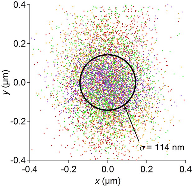
Optical tracking error.
Position data recorded for 1 min each from 4 dead worms spotted by the usual procedure. Under these conditions the stage is stationary. Data from each worm are shown in a different color. The circle encloses 1 standard deviation of the combined 2-D distribution. Optical tracking is more precise than the resolution of the stage position encoder, and thus does not limit the overall resolution of the position measurement.

The worm’s search behavior closely resembles a Brownian random walk on time scales longer than 10 s, but not on shorter time scales.
(A) the velocity autocorrelation function () averaged across the 5 wild-type cohorts shows that movements become uncorrelated after ~10 s, primarily as a result of random reorientation during transitions from reverse to forward motion. The period of the damped oscillations in corresponds to the period of sinusoidal undulations during locomotion. (B) The observed linear increase in mean-squared distance travelled with time (black; mean ± sem, averaged data from all wild-type worms) shows that on this time scale search behavior approximates a Brownian random walk. (C) At shorter times the observed (black) relation curves upward because worms travel in relatively straight lines during runs. Assuming that the behavior is stationary over the 10 min observation period, the dependence of on can be calculated from the velocity autocorrelation function (red curves in B and C):
where denotes statistical expectation (eq. 2.5.12 of Boon and Yip, 1980). Thus, the worm’s movements approximate Brownian motion on a time scale that is longer than the persistence of the velocity autocorrelation, but not at shorter times.
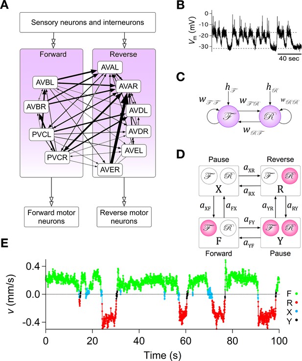
Assumptions with supporting data for the Stochastic Switch Model.
(A) Connectivity of forward and reverse command neurons. Arrows with single heads are monosynaptic connections inferred from the C. elegans connectome (White et al., 1986; Varshney et al., 2011) line thickness is proportional to the number of presynaptic specializations seen in the reconstruction of each pairwise connection. Open, double-headed arrows indicate synaptic pathways from or to the indicated pool of neurons outside the network. (B) Voltage recording from the command neuron AVA in the absence of injected current. In this neuron, quasi-stable membrane potentials are seen at -17 and -32 mV. These results differ from previously published AVA recordings, which were made in the presence of hyperpolarizing current (5–10 pA) that kept the membrane potential near -55 mV (Lindsay et al., 2011). (C) Neuronal representation of the Stochastic Switch Model. Forward and reverse command neurons are represented as single binary neuron-like units and , respectively. Arrows depicting cross connections (, ) represent functional (net mono- and polysynaptic) connections between forward and reverse units. Self-connections (, ) represent synaptic connections between neurons comprising a given unit, voltage dependent currents in these neurons, and polysynaptic recurrent pathways involving non-command neurons. Downward arrows (, ) represent the combined effects of input from presynaptic neurons, including sensory neurons, and neuromodulation. (D) Markov model representation of the command neuron network. The color of a unit indicates its state of activation (red on, white off). In addition to the forward state F and the reverse state R, there are two pause states, X and Y. Arrows, with their associated rate constants, indicate transitions in which a single unit changes state. Transitions in which two units change state simultaneously have probability zero because single-unit transitions are assumed to be statistically independent. (E) The most likely sequence of states in the hidden Markov model (computed using the Viterbi algorithm) for a representative data segment.
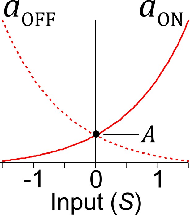
Effects of synaptic input on transition rates in stochastic units and .
Rate constants are exponential functions of the unit’s net synaptic input S. Excitatory input increases the on rate and decreases the off rate, whereas inhibitory input has the opposite effect. When synaptic input equals zero, the unit switches stochastically between on and off states with rate constant A.
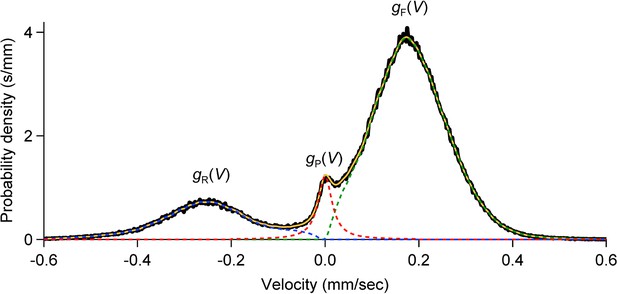
Velocity distributions in forward, reverse and pause states.
For each cohort, the velocity distribution (black; binwidth 2 µm/s) was smoothed by 10 passes of a 1-2-1 binomial smoothing algorithm, then separated into three overlapping velocity distributions: (dashed green), (dashed blue), (dashed red).
For we used a Cauchy distribution (half width 18 µm/s) scaled to fit . We estimated and by subtracting from and restricting the F and R distributions to positive and negative velocities, respectively. The sum is shown in solid orange.

Cumulative dwell time distributions in states F, R, X and Y.
Comparisons between cumulative dwell time distributions (solid lines) and the exponential distributions predicted by the hidden Markov model (, where is the mean dwell time in state ; Table 1). The observed dwell times were tabulated from the most likely sequence of states obtained using the Viterbi algorithm. The origin on the time axis corresponds to one frame.

Fate diagram of the model.
The system typically cycles clockwise through states F, X, R, Y, with state F frequently interrupted by FXF transitions, leading to state sequences of the form …(FX)nRY(FX)nRY…. Nearly unidirectional transitions out of a given state are shown by red arrows; blue arrows indicate nearly equiprobable transitions. The width of the arrows and the numbers beside them show the probability that the transition out of the state at the tail of the arrow is into the state at the head. The area of each circle is proportional to the probability of the corresponding state (Table 1, column A).
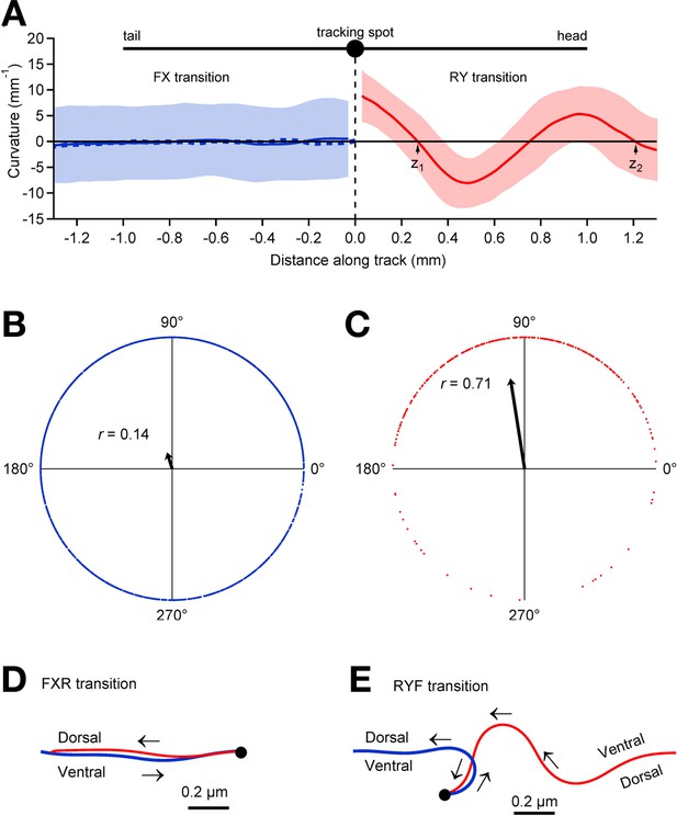
Relationship between pauses and posture.
(A) Average track curvature upon entry in to the pause state in wild type worms. Prior to computing curvature, tracks of individual worms were mirror-imaged as needed such that positive curvature corresponds to a ventral bend. Tracks in the vicinity of pause events were aligned according to the location of the tracking spot in the pause state, converted to curvature, then averaged over all FX transitions (solid blue line; n = 1907), and all RY transitions (red; n = 295) for which the track length was >1.5 mm; shading shows ± 1 S.D. The trace depicts the curvature of the worm posterior to the tracking spot at the end of forward movement (FX transitions) and anterior to the tracking spot at the end of reverse movement (RY transitions). The dashed blue line shows the average curvature at FXR transitions (i.e., excluding FXF stutters). (B) Locomotory phases at which FX transitions occurred, plotted as blue dots on the unit circle. The phase at each FX transition was computed as , where and are the positions of the two downward zero crossings of curvature preceding the pause as indicated in panel A, right. The uniform distribution of points around the circle, and therefore the small magnitude of the vector strength (; arrow), shows that there was only a small (but statistically significant) phase preference at the end of forward motion (; Rayleigh test). (C) Same as B, but for RY transitions. Vector strength is large (), indicating a strong tendency to end reverse runs at a particular phase (), with a ventral bend in the middle of the body. (D) Average posture at FXR transitions, calculated by integrating the average curvature, computed over all tracks that persisted for >1.5 mm in state F before the pause and >1 mm in state R after the pause. Arrows indicate direction of motion along the track (blue, forward; red, reverse). FXR transitions were typically a simple reversal along the same track. (E) Same as D but for RYF transitions that persisted for >1.5 mm in state R before the pause and >1 mm in state F after the pause. RYF transitions at the end of reverse runs that persisted for >1.5 mm were usually associated with a ventral bend that resulted in a ~180° change of direction as previously described (Gray et al., 2005).
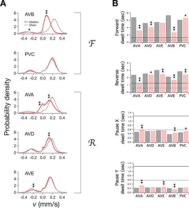
Ablation of command neurons.
(A) Velocity distribution of ablated cohorts (red) compared to sham operated controls (grey) when the indicated command neuron was killed. Stars indicate significant reduction in velocity for the indicated peak (p<0.05 without () or with () correction for multiple comparisons; Table 3). (B) Dwell times in F, R, and P in ablated (red) and sham operated animals (grey). Stars indicate significant differences from sham (as defined in Table 4). Horizontal lines indicate the estimated range of , the dwell time in the uncoupled state. Each group of ablated animals was tested in parallel with a distinct set of sham operated controls to minimize the effects of variation between populations. Error bars for dwell times are not shown because statistical significance was calculated using the likelihood ratio test (see Table 4 legend), which does not generate sem estimates, and calculation of confidence intervals would have required an excessive amount of computation time. Stars indicate p<0.05 without () or with () correction for multiple comparisons (Table 4).
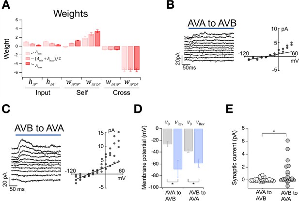
The Stochastic Switch Model correctly predicts the sign and strength of synaptic connections.
(A) Synaptic weights (mean ± sem, n = 5 cohorts) from maximum likelihood fits to velocity data from wild type worms. (B, C) Left, synaptic current in AVB or AVA when the indicated presynaptic neuron was photoactivated (blue line). Right, mean synaptic current during the first 100 ms of the stimulus plotted against holding potential in the postsynaptic neuron (I-V curve). Lines show linear fits to the data at negative holding potentials which were used to estimate . (D), Zero-current holding potential and reversal potential of synaptic currents (mean ± sem) in the indicated postsynaptic neuron (paired t-tests: AVA to AVB, p= 0.043, n = 9; AVB to AVA, p= 0.019, n = 17). (E), Scatter plot of synaptic currents recorded at a holding potential of -15 mV (unpaired t-test: p= 0.010, n ≥ 25).
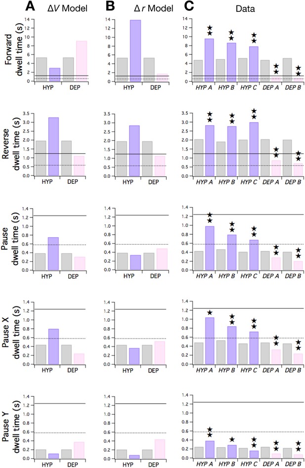
Predicted and observed effects of HYP and DEP mutations on dwell times.
(A) Predicted effects of changes in membrane potential. (B ) Predicted effects of changes in input resistance. (C) Dwell times in F, R, and P for cohorts of HYP mutants, DEP mutants, and wild type animals. Stars indicate significant change in dwell time (p<0.05 without () or with () correction for multiple comparisons; Table 6). In A-C wild type dwell times are indicated by gray bars. Horizontal lines indicate the estimated range of , the dwell time in the uncoupled state. In the ΔV model, terms were made more negative to model HYP mutants and more positive to model DEP mutants by subtracting or adding a constant = 0.6; qualitatively similar results were obtained for 0 < ≤ 0.8. In the Δr model, and terms were scaled by (1 + f) to model HYP mutants and by (1 - f) to model DEP mutants, with f = 0.6; qualitatively similar results were obtained for 0 < f ≤ 1. Strains, HYP A: DA572 eat-4(ad572); HYP B: MT6308 eat-4(ky5); HYP C: KP4 glr-1(n2461); DEP A: VM1136 lin-15(n765); akIs9 [lin-15(+), Pglr-1::GLR-1(A/T)]; DEP B: VM188 lin-15(n765); akEx52[lin-15(+), Pnmr-1::GLR-1(A/T)].
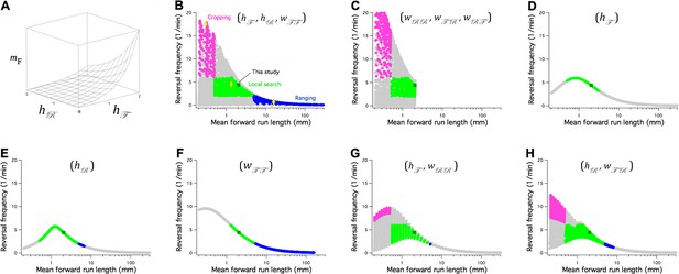
The Stochastic Switch Model accounts for the three main modes of random search in C. elegans.
(A) Plot of mean forward run length versus the weights and , illustrating a minimal model of search-scale regulation. (B-H) Calculated effects on search mode of the weights indicated in parentheses. The frequency of reversals () is plotted against while these three weights are scanned from -6 to 6 weight units in steps of 0.4. Each point was categorized as cropping (magenta), local search (green), ranging (blue), or indeterminate (grey) according to value of and , and whether or not the associated value of (not shown) indicated a short or long reversal; see Materials and methods for definitions of search modes. Yellow diamonds mark the scanned points modeled in Figure 8—figure supplement 1. = 1 Hz; similar results were obtained for and (Table 7).
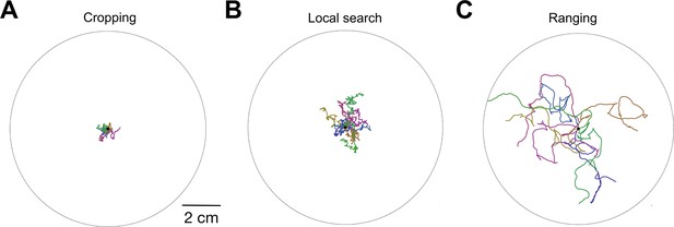
Simulated worm tracks illustrating cropping, local search, and ranging as defined in the model.
( A-C ) Simulated time is 600 sec with four replicated per panel, each in a different color. ; similar results were obtained for .
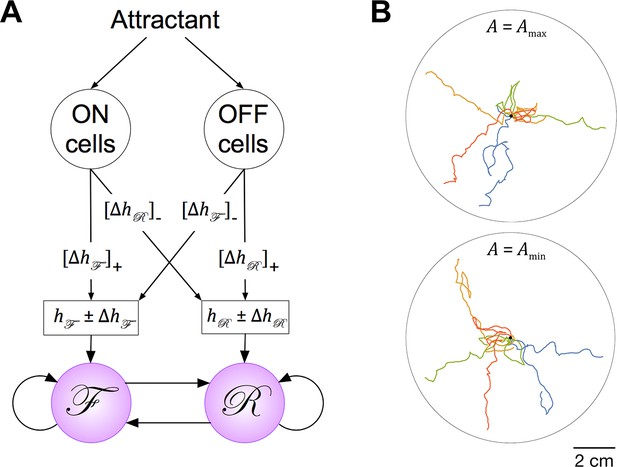
Extension of the Stochastic Switch Model to chemotaxis.
(A) Circuitry. Behavioral state (F, R, or P) was determined by a modified version of the Stochastic Switch Model in which on and off chemosensory neurons regulated the values of the inputs to the network. During movement up the gradient, the activation states of the on and off cells were set to 1 and 0, respectively, such that and , where and are the values of the inputs to the network during local search (Table 2). Conversely, during movement down the gradient, the on and off activation states, and the signs of , were reversed. In the tracks shown, and were 2.6, the value that optimized chemotaxis performance given the speed of the model worm and standard deviation of the gradient. (B) Simulated chemotaxis. The concentration gradient of chemical attractant was modeled as a two dimensional Gaussian (std. dev. = 1.6 cm) originating at the center of a circular arena. Similar tracks were obtained across the full range of values of A, the fundamental time scale of the model.
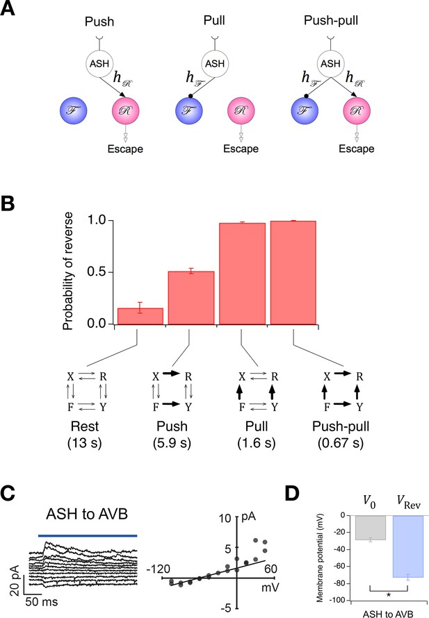
Extension of the Stochastic Switch Model to deterministic behaviors.
(A) Three functional circuit motifs for deterministic escape behavior initiated by the nociceptive neuron ASH. (B) Predicted steady-state probability of reversal behavior in the resting state and the activated state of the three motifs shown in A. Plotted values are means across the five wild type cohorts shown in Figure 1F. Error bars are ± sem. Numbers in parenthesis are predicted mean first latency to a reversal response. (C) Left, synaptic current in AVB when ASH was photoactivated (blue line). Right, mean synaptic current during the first 100 ms of the stimulus plotted against holding potential in AVB. The line is fit to the data at negative holding potentials. (D) Mean zero-current holding potential and mean reversal potential of synaptic currents (± sem) in AVB (paired t-test: p= 0.013, n = 4).
Videos
Forward-Pause-Forward transition.
The worm is crawling on a foodless agar plate. The microscope stage moves continuously to keep the tracking spot near the center of the frame. Stage movement can be assessed by monitoring the white streaks in the background, which are segments of the worm's track at earlier times. Behavioral state is indicated in the upper left corner of the frame. The indicated behavioral transition is shown at normal speed, and slowed down by a factor of 5. The worm is paused when the tracking spot is stationary relative to the streaks.
Reverse-Pause-Reverse transition.
https://doi.org/10.7554/eLife.12572.007Forward-Pause-Reverse transition.
https://doi.org/10.7554/eLife.12572.008Reverse-Pause-Forward transition.
https://doi.org/10.7554/eLife.12572.009Tables
Maximum likelihood fits of transition rates in wild type C. elegans.
Each cohort was fitted separately; values are expressed as mean ± sem (n = 5 cohorts). Data from wild type cohorts were obtained on the same days as the experimental cohorts for which they served as controls (Tables 3 and 4), but experimental cohorts in this study were separated by weeks to months. All transition rates were constrained to be ≥0. Transition rates that were calculated using the synaptic constraints (Equation 35) are shaded orange; other constrained values are shaded grey. Mean dwell times and state probabilities were calculated from the transition rates. Column A shows fits using the standard model, which has 8 rate constants with two synaptic constraints, resulting in 6 free parameters that determine the 6 synaptic weights (Figure 2C,D; Materials and methods Equations 31–35). Column B shows fits to a model that has only one pause state (X); this model was derived from the standard model by imposing two more constraints: , yielding 4 free parameters. To allow comparison of models A and B by the likelihood ratio test, which requires tht model B be a special case of model A, and were set slightly >0 (10-10 s-1), thereby avoiding infinite values for and when applying the synaptic constraints, while maintaining a vanishingly small probability of being in state Y ( 10-18). The loge likelihood (summed over the 5 cohorts) for model B was 1854 less than for model A, with 30 degrees of freedom for model A (6 per cohort × 5 cohorts) and 20 degrees of freedom for model B (4 per cohort × 5 cohorts). Applying the likelihood ratio test, the difference was highly significant (p<10-100; p=Chi-squared(2L, df), where L = 1854 and df = 30–20 =10. Model C is the most general 3-state (F, R, P) model, which allows all six transitions between the three states. The fitted transition rates for model C were nearly identical to model B. Likelihood values are relative to model A.
| A | B | C | |
|---|---|---|---|
| 2 pause states6 free parameters | 1 pause state4 free parameters | 1 pause state6 free parameters | |
| Δ loge likelihood | 0 | -1854 | -1836 |
| Degrees of freedom | 30 | 20 | 30 |
| mean ± sem (n = 5) | mean ± sem (n = 5) | mean ± sem (n = 5) | |
| (s-1) | 1.201 ± 0.099 | 1.019 ± 0.085 | 1.008 ± 0.090 |
| (s-1) | 1.115 ± 0.087 | 1.915 ± 0.152 | 1.914 ± 0.152 |
| (s-1) | 0.025 ± 0.008 | 0.507 ± 0.013 | 0.507 ± 0.013 |
| (s-1) | 0.490 ± 0.015 | 10-10 | |
| (s-1) | 0.182 ± 0.007 | 0.198 ± 0.009 | 0.196 ± 0.008 |
| (s-1) | 0.007 ± 0.002 | 10-10 | |
| (s-1) | 0.411 ± 0.019 | >109 | |
| (s-1) | 4.575 ± 0.533 | >109 | |
| (s-1) | 0.001 ± 0.001 | ||
| (s-1) | 0.000 ± 0.000 | ||
| (s) | 5.329 ± 0.245 | 5.096 ± 0.235 | 5.135 ± 0.227 |
| (s) | 1.945 ± 0.043 | 1.975 ± 0.049 | 1.976 ± 0.049 |
| (s) | 0.441 ± 0.032 | 0.349 ± 0.026 | 0.351 ± 0.027 |
| (s) | 0.208 ± 0.019 | <10-9 | |
| 0.762 ± 0.015 | 0.7641 ± 0.015 | 0.764 ± 0.014 | |
| 0.158 ± 0.007 | 0.158 ± 0.007 | 0.155 ± 0.007 | |
| 0.063 ± 0.006 | 0.081 ± 0.008 | 0.080 ± 0.008 | |
| 0.017 ± 0.002 | <10-18 |
Synaptic weights derived from the transition rate constants.
The rate constants were taken from Table 1, column A. Two values of the fundamental switching time, A, corresponding to the minimum (0.40 Hz) and maximum (0.86 Hz) values consistent with the ablation results were used in Materials and methods, Equations 36–38 to calculate the corresponding synaptic weights.
| 0.4 Hzmean ± sem (n = 5) | 0.86 Hzmean ± sem (n = 5) | |
|---|---|---|
| 1.01 ± 0.08 | 0.25 ± 0.08 | |
| 1.09 ± 0.08 | 0.32 ± 0.08 | |
| -5.40 ± 0.43 | -5.40 ± 0.43 | |
| -0.81 ± 0.06 | -0.81 ± 0.06 | |
| -0.22 ± 0.06 | 1.31 ± 0.06 | |
| 1.90 ± 0.33 | 3.43 ± 0.33 |
Effects of command neuron ablations on undulation frequency, forward velocity and reverse velocity.
Values were computed separately for each worm and are shown as mean ± sem (n = 19–29 ). Undulation frequency was estimated as one-half of the reciprocal of the time of the first local minimum in the heading autocorrelation function. All p-values are from two-tailed t-tests and are shown without correction for multiple comparisons. Blue denotes significance at p<0.05. Red denotes significance at p<0.05 after Bonferroni correction for 15 comparisons.
| Undulation frequency (Hz) | Forward velocity (μm/s) | Reverse velocity (μm/s) | ||||||||
|---|---|---|---|---|---|---|---|---|---|---|
| Neuron | Class | Sham | Ablated | p < | Sham | Ablated | p < | Sham | Ablated | p < |
| AVB | Forward | 0.355 ± 0.009 | 0.230 ± 0.007 | 236 ± 6 | 109 ± 4 | -327 ± 7 | -302 ± 8 | |||
| PVC | Forward | 0.283 ± 0.011 | 0.290 ± 0.010 | 0.5 | 187 ± 7 | 192 ± 7 | 0.7 | -253 ± 8 | -248 ± 6 | 0.7 |
| AVD | Reverse | 0.270 ± 0.008 | 0.236 ± 0.008 | 173 ± 6 | 141 ± 5 | -243 ± 4 | -229 ± 5 | 0.06 | ||
| AVA | Reverse | 0.302 ± 0.005 | 0.254 ± 0.009 | 195 ± 5 | 155 ± 7 | -293 ± 7 | -69 ± 3 | |||
| AVE | Reverse | 0.264 ± 0.007 | 0.256 ± 0.008 | 0.6 | 165 ± 4 | 160 ± 5 | 0.5 | -235 ± 4 | -211 ± 6 | |
Effects of command neuron ablations on model parameters.
The sign of the change (Δ) caused by the ablation is shown as “+” if the value moved away from 0, “–” if the value moved towards 0. Significance was determined using the likelihood ratio test (Weisstein, Eric W. "Likelihood Ratio." From MathWorld--A Wolfram Web Resource. http://mathworld.wolfram. com/LikelihoodRatio.html), which is based on the reduction in likelihood caused by constraining one of the parameters to have the same value in both the ablated cohort and the corresponding sham cohort. The unconstrained fit thus had 12 free parameters (6 for each of the 2 cohorts being compared), while the constrained fit had 11 free parameters. For example, to test the significance of the change in the mean dwell time in the pause state ( caused by ablation of the AVA neuron pair, two cohorts (ablated and sham) were grown and tested under identical conditions. The ln likelihood with 12 free parameters was found to be 894794.075. When was constrained to be the same for both cohorts, the ln likelihood for the 11 parameter fit was found to be 894784.676. The test statistic was assumed to come from a chi-squared distribution with one degree of freedom, which yielded (shown in the table as ). The constrained fitting process was repeated in turn for each ablation/sham pair for each of the 9 rows shown in the table. All p-values are shown without correction for multiple comparisons. Blue denotes significance at p<0.05. Red denotes significance at p<0.05 after Bonferroni correction for 27 comparisons
| REVERSE | FORWARD | |||||||||||||||||||
|---|---|---|---|---|---|---|---|---|---|---|---|---|---|---|---|---|---|---|---|---|
| AVE | AVD | AVA | AVB | PVC | ||||||||||||||||
| Sham | Ablate | ∆ | p< | Sham | Ablate | ∆ | p< | Sham | Ablate | ∆ | p< | Sham | Ablate | ∆ | p< | Sham | Ablate | ∆ | p< | |
| (s) | 5.455 | 5.221 | – | 0.2 | 5.158 | 4.081 | – | 6.730 | 3.143 | – | 7.289 | 2.642 | – | 6.058 | 6.558 | + | ||||
| (s) | 3.019 | 2.436 | – | 2.540 | 2.367 | – | 2.359 | 1.243 | – | 2.127 | 1.681 | – | 2.842 | 2.396 | – | |||||
| (s) | 0.548 | 0.548 | – | 1 | 0.514 | 0.520 | + | 0.6 | 0.480 | 0.582 | + | 0.370 | 0.437 | + | 0.457 | 0.508 | + | |||
| (s) | 0.229 | 0.263 | + | 0.229 | 0.241 | + | 0.07 | 0.214 | 0.331 | + | 0.197 | 0.144 | – | 0.220 | 0.226 | + | 0.5 | |||
| (s) | 0.495 | 0.496 | + | 1 | 0.460 | 0.468 | + | 0.5 | 0.437 | 0.510 | + | 0.331 | 0.416 | + | 0.410 | 0.457 | + | |||
| 0.720 | 0.747 | + | 0.723 | 0.689 | – | 0.809 | 0.704 | – | 0.818 | 0.745 | – | 0.749 | 0.787 | + | ||||||
| 0.192 | 0.158 | – | 0.188 | 0.203 | + | 0.122 | 0.137 | + | 0.129 | 0.120 | – | 0.2 | 0.181 | 0.139 | – | |||||
| 0.073 | 0.078 | + | 0.07 | 0.072 | 0.088 | + | 0.058 | 0.113 | + | 0.041 | 0.125 | + | 0.056 | 0.061 | + | 0.2 | ||||
| 0.014 | 0.017 | + | 0.017 | 0.020 | + | 0.011 | 0.046 | + | 0.012 | 0.010 | – | 0.014 | 0.013 | – | 0.5 | |||||
Effects of mutations on mean undulation frequency, mean forward velocity and mean reverse velocity.
Values were computed separately for each worm and are shown as mean ± sem (n = 25–31). Undulation frequency was estimated as one-half of the reciprocal of the time of the first local minimum in the heading autocorrelation function. All p-values are from two-tailed t-tests and are shown without correction for multiple comparisons. Blue denotes significance at p<0.05. Red denotes significance at p<0.05 after Bonferroni correction for 15 comparisons.
| Undulation frequency (Hz) | Forward velocity (μm/s) | Reverse velocity (μm/s) | ||||||||
|---|---|---|---|---|---|---|---|---|---|---|
| Genotype | Class | Wild type | Mutant | p < | Wild type | Mutant | p < | Wild type | Mutant | p < |
| eat-4(ad572) | HYP A | 0.272 ± 0.011 | 0.222 ± 0.007 | 156 ± 5 | 122 ± 4 | -228 ± 5 | -236 ± 9 | 0.5 | ||
| eat-4(ky5) | HYP B | 0.317 ± 0.011 | 0.256 ± 0.009 | 184 ± 7 | 143 ± 6 | -262 ± 10 | -271 ± 7 | 0.5 | ||
| glr-1(n2461) | HYP C | 0.294 ± 0.008 | 0.291 ± 0.010 | 0.9 | 158 ± 5 | 166 ± 6 | 0.3 | -236 ± 6 | -236 ± 5 | 1 |
| glr-1::glr-1(A/T) | DEP A | 0.272 ± 0.011 | 0.642 ± 0.029 | 156 ± 5 | 112 ± 5 | -228 ± 5 | -143 ± 5 | |||
| nmr-1::glr-1(A/T) | DEP B | 0.294 ± 0.008 | 0.695 ± 0.037 | 158 ± 5 | 138 ± 5 | -236 ± 6 | -144 ± 5 | |||
Effects of mutations on model parameters.
Significance was determined using the likelihood ratio test as described in Table 4. The sign of the change (Δ) caused by the mutation is shown as “+” if the value moved away from 0, “–” if the value moved towards 0. All p-values are shown without correction for multiple comparisons. Blue denotes significance at p<0.05. Red denotes significance at p<0.05 after Bonferroni correction for 27 comparisons.
| HYP | DEP | |||||||||||||||||||
|---|---|---|---|---|---|---|---|---|---|---|---|---|---|---|---|---|---|---|---|---|
| HYP A: eat-4(ad572) | HYP B: eat-4(ky5) | HYP C: glr-1(n2461) | DEP A: glr-1::glr-1(A/T) | DEP B: nmr-1::glr-1(A/T) | ||||||||||||||||
| Control | Mutant | p < | Control | Mutant | ∆ | p< | Control | Mutant | ∆ | p< | Control | Mutant | ∆ | p< | Control | Mutant | ∆ | p< | ||
| (s) | 4.771 | 9.564 | + | 4.956 | 8.643 | + | 5.181 | 7.871 | + | 4.771 | 0.940 | – | 5.181 | 0.742 | – | |||||
| (s) | 2.043 | 2.821 | + | 1.910 | 2.769 | + | 2.018 | 3.004 | + | 2.045 | 0.875 | – | 2.018 | 0.709 | – | 9 | ||||
| (s) | 0.481 | 1.040 | + | 0.529 | 0.844 | + | 0.459 | 0.727 | + | 0.482 | 0.328 | – | 0.460 | 0.235 | – | |||||
| (s) | 0.247 | 0.382 | + | 0.238 | 0.290 | + | 0.221 | 0.164 | – | 0.247 | 0.097 | – | 0.221 | 0.079 | – | |||||
| (s) | 0.428 | 0.982 | + | 0.466 | 0.793 | + | 0.409 | 0.677 | + | 0.428 | 0.286 | – | 0.409 | 0.204 | – | |||||
| 0.729 | 0.839 | + | 0.734 | 0.832 | + | 0.755 | 0.785 | + | 0.728 | 0.410 | – | 0.755 | 0.407 | – | ||||||
| 0.177 | 0.062 | – | 0.167 | 0.079 | – | 0.161 | 0.135 | – | 0.177 | 0.389 | + | 0.161 | 0.404 | + | ||||||
| 0.073 | 0.090 | + | 0.077 | 0.081 | + | 0.3 | 0.067 | 0.073 | + | 0.073 | 0.164 | + | 0.067 | 0.151 | + | |||||
| 0.022 | 0.009 | – | 0.021 | 0.008 | – | 0.018 | 0.007 | – | 0.022 | 0.037 | + | 0.018 | 0.037 | + | ||||||
Regulation of search mode.
The weights in each subspace were scanned from -6 to 6 weight units in steps of 0.4 with or . The letter x means that the indicated search mode was present for at least one point in the subspace when and when ; the letters y and z mean that the mode was present only when or , respectively. See Materials and methods for definitions of search modes. Control-point weights as defined by the theoretical relationship between weights and search scale (Equation 5) are shown in bold. Only the three-weight subspaces are sufficient for producing all three search modes and full coverage of the plane defined by reversal frequency and plane as shown in Figure 8.
| Subspace | Ranging | Coverage | ||
|---|---|---|---|---|
| ⋅ ⋅ ⋅ | ||||
| x | ⋅ ⋅ ⋅ | |||
| x | ⋅ ⋅ ⋅ | |||
| . . . | ||||
| . . . | ||||
| . . . | ||||
| , | . . . | |||
| , | . . . | |||
| , | . . . | |||
| , | . . . | |||
| , | . . . | |||
| , | . . . | |||
| , | . . . | |||
| , | . . . | |||
| , | . . . | |||
| , | . . . | |||
| , | . . . | |||
| , | . . . | |||
| , | ....... | |||
| , | . . . | |||
| , | ....... | |||
| , , | ....... | |||
| , , | ....... | |||
| , , | ....... | |||
| , , | ....... | |||
| , , | ....... | |||
| , , | ....... | |||
| , , | ....... | |||
| , , | ....... | |||
| , , | ....... | |||
| , , | ....... | |||
| , , | ....... | |||
| , , | ....... | |||
| , , | ....... | |||
| , , | ....... | |||
| , , | ....... | |||
| , , | ....... | |||
| , , | ....... | |||
| , , | ....... | |||
| , , | ....... | |||
| , , | ....... |


