Dynamic curvature regulation accounts for the symmetric and asymmetric beats of Chlamydomonas flagella
- Max Planck Institute for the Physics of Complex Systems, Germany
- Yale University, United States
Figures
Figure 1
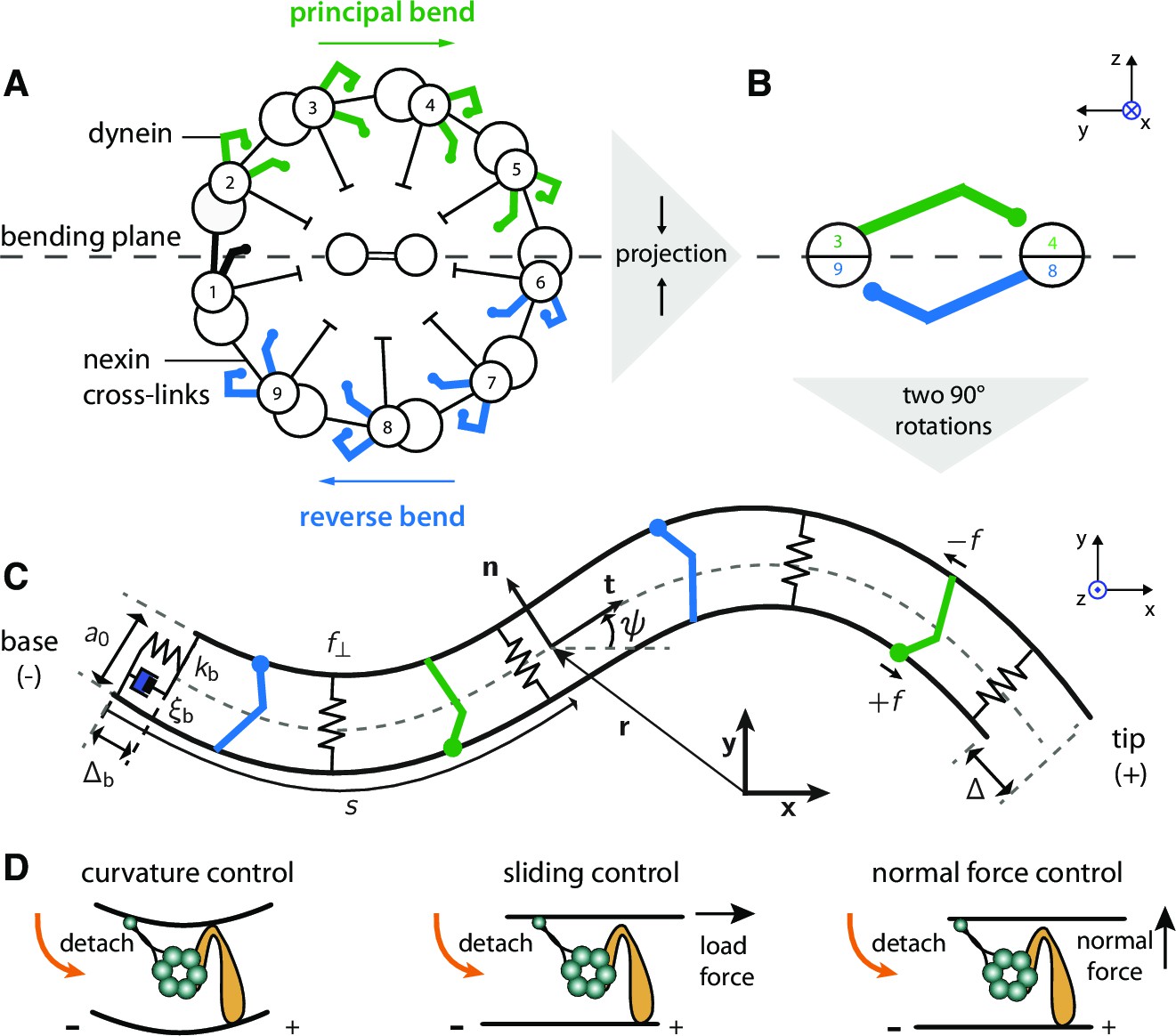
Two-dimensional model of the axoneme and mechanisms of dynein regulation.
(A) Cross-section of an axoneme, as seen from the basal end looking towards the distal tip. The numbering of the doublets follows the convenstion for Chlamydomonas (Hoops and Witman, 1983). The green dyneins bend the axoneme such that the center of curvature is to the right. (B) The projection of the cross section onto two filaments to form the two-dimensional model. The green and blue motors bend the filament pair in opposite directions. (C) Two-dimensional model of the axoneme, as seen in the bending plane, . The two filaments are constrained to have spacing . The point at arc-length has position vector (relative to the origin), tangent vector , normal vector , and tangent angle with respect to the horizontal axis of the lab-frame . Dyneins on the upper filament (green) have microtubule-binding domains (MTBs, denoted by filled circles) that walk along the lower filament towards the base and produce a (tensile) force density on the lower filament. This force slides the lower filament towards the distal end. The dyneins on the opposite filament (blue) create sliding (and bending) forces in the opposite direction. The local sliding displacement is given by , and the sliding at the base is . The sign convention is defined in Figure 10 and Appendix 4. The springs between the filaments oppose filament separation by the normal force, . The spring and dashpot at the base consitute the basal compliance, with stiffness and friction coefficient . (D) Schematic of dynein regulation mechanisms. In curvature control the dynein MTB detaches due to an increase in curvature. In sliding control detachment is enhanced by a tangential loading force, and in normal force control the normal force, which tends to separate the filaments, enhances detachment. Signs indicate doublet polarity.
Figure 2
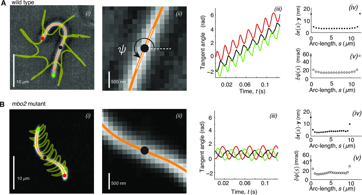
High precision tracking of isolated, reactivated axonemes.
Panel A corresponds to Chlamydomonas wild type axonenes, panel B to mbo2 mutant axonemes. (A) (i) Inverted phase-contrast image of a wild type axoneme. The orange curve represents the tracked centerline. The points depict the basal end (red), the distal end (green) and the center position (black) of the axoneme. The yellow line depicts the trajectory of the basal end, which is the leading end during swimming (Geyer, 2012). (ii) Same image as in Ai, magnified around the center region. The tangent angle is defined with respect to the lab frame. (iii) Tangent angle at three different arc-length positions (depicted in Ai) as a function of time. The linearly increasing tangent angle corresponds to a counter-clockwise rotation of the axoneme during swimming. Mean uncertainty measured over 1000 adjacent frames of the position (iv) (the error gives a similar result) and the tangent angle in (v). (B) is analogous to (A), but for mbo2 mutant axonemes.
Figure 3
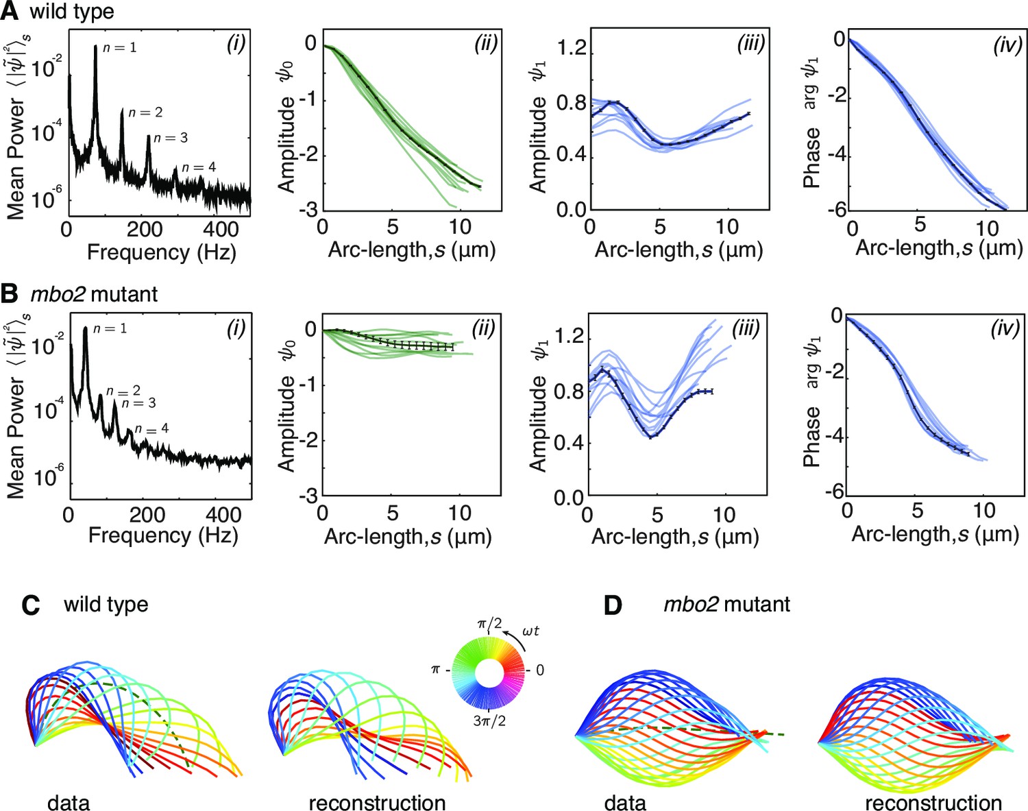
Fourier decomposition of the beat.
Panel A shows the Fourier decomposition of the waveform of wild type axonemes, panel B the decomposition of the mbo2 axoneme waveform. (A) (i) Power spectrum of the tangent angle averaged over arc-length. The fundamental mode () and three higher harmonics () are labeled. (ii) Angular representation of the static () mode as a function of arc-length. The approximately constant slope indicates that the static curvature is close to constant . (iii) The amplitude and phase (argument) of the fundamental mode are shown in iii and iv, respectively. The approximately linear decrease in phase indicates steady wave propagation. The data of a representative axoneme is highlighted in the panels ii–iv, with error bars indicating the standard error of the mean calculated by hexadecimation. (B) Equivalent plots to (A) for mbo2 axonemes. (C) Beat shapes of one representative beat cycle of the wild type axoneme highlighted in panel A (left panel, data) and shapes reconstructed from the superposition of the static and fundamental modes, neglecting all higher harmonics. The progression of shapes through the beat cycle is represented by the rainbow color code (see inset). (D) Same as (C) for an mbo2 mutant axoneme.
Figure 4

Comparison of theoretical and experimental beating patterns.
(A) Comparison of the theoretical (lines) and experimental (dots) beating patterns of a typical wild type axoneme. The real and imaginary part of the first mode of the tangent angle is plotted for beats resulting from sliding control, curvature control, and normal force control. (B) Analogous to (A) for mbo2. Note that here also curvature control and normal force control provide good agreement, but not sliding control. (C) and (D) Theoretical and experimental shape reconstruction in position space for the wild type and mbo2 beats under curvature control.
Figure 5
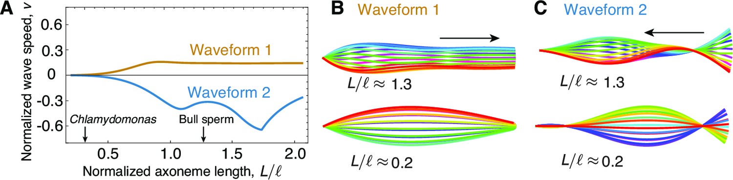
The role of length in sliding-regulated beats.
(A) Wave speed versus relative length of the first two unstable waveforms of a freely swimming axoneme regulated by sliding. For short lengths, in the range of Chlamydomonas, the modes lose directionality and become standing waves. Long axonemes have directional waves that can travel either forward, as in waveform 1,or backwards, as in waveform 2. (B) Two examples of waveform 1 for long (top) and short (bottom) axonemes. Note that the short axonemes have standing waves. See (Sartori, 2015) for more details. (C) Beating patterns of waveform 2 for a long (top) and short (bottom) axonemes. In B and C arrows denote direction of wave propagation.
Figure 6
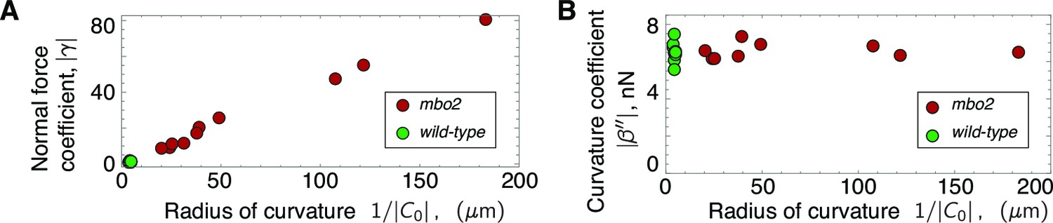
Scaling of response coefficients with static curvature.
(A) Because the normal force is proportional to the static curvature , the normal force response coefficient is inversely proportional to the curvature. Red symbols are mbo2 and green symbols are wild type. (B) The curvature control response coefficient is independent of the static curvature, and remains constant even for a fifty-fold change in static curvature.
Figure 7
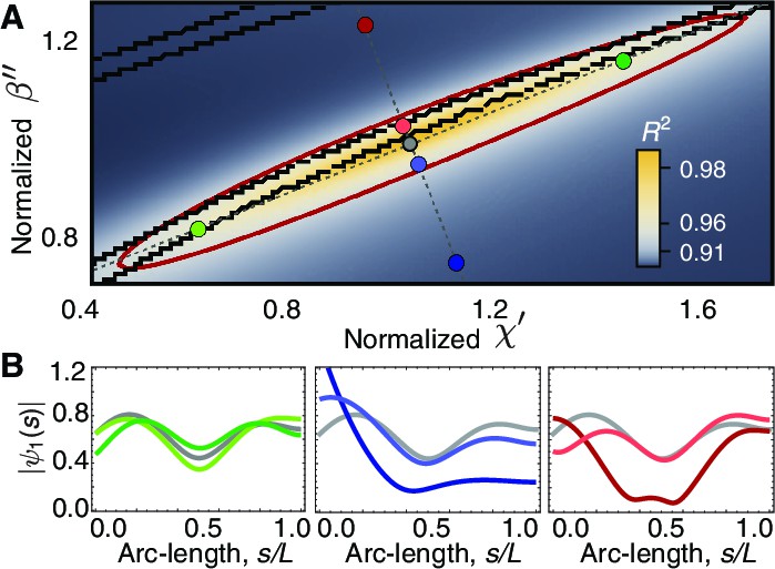
Phase space of curvature control.
(A) Heat map of the mean-square distance between the theoretical and a reference experimental beat as a function of the sliding response coefficient and the curvature response coefficient . The ellipsoid delimits the region with . Each pair of nearby black lines delimits a region with a passive base. Moving along the long axis (green circles) affects the amplitude dip in the midpoint of the axonemem, left panel in (B). Moving along the short axis towards the region of active base results in waveforms with a large amplitude at the base (blue and red circles), central and right panels in B. The axis in A is normalized by the reference fit, such that corresponds to the highest value of .
Figure 8
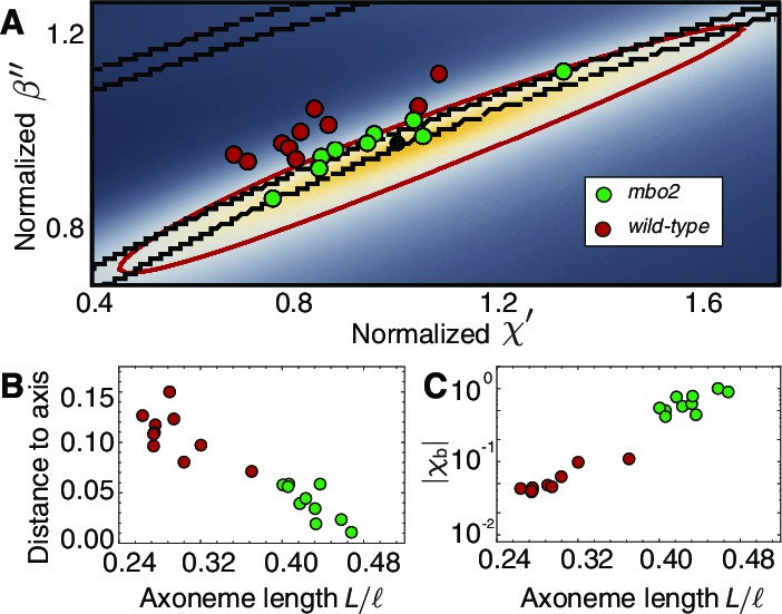
Axonemal variability in phase space.
(A) Circles represent values obtained from fits for each of the axonemes, green corresponds to wild type and red to mbo2. In the background we have the same heat map as in Figure 7. Note that mbo2 points lie away from wild type circles in the direction of the short axis of the ellipse. All values are normalized by those of the reference fit used also to normalize the heat map axis. (B) The distance of the circles to the long axis of all fits shows a clear correlation with normalized axonemal length. Note also that mbo2 axonemes are systematically shorter than wild type axonemes. (C) The basal compliance () also correlates with the normalized length, resulting in a high value for wild type axonemes, which are longer. The values are normalized by the value for a reference axoneme.
Figure 9
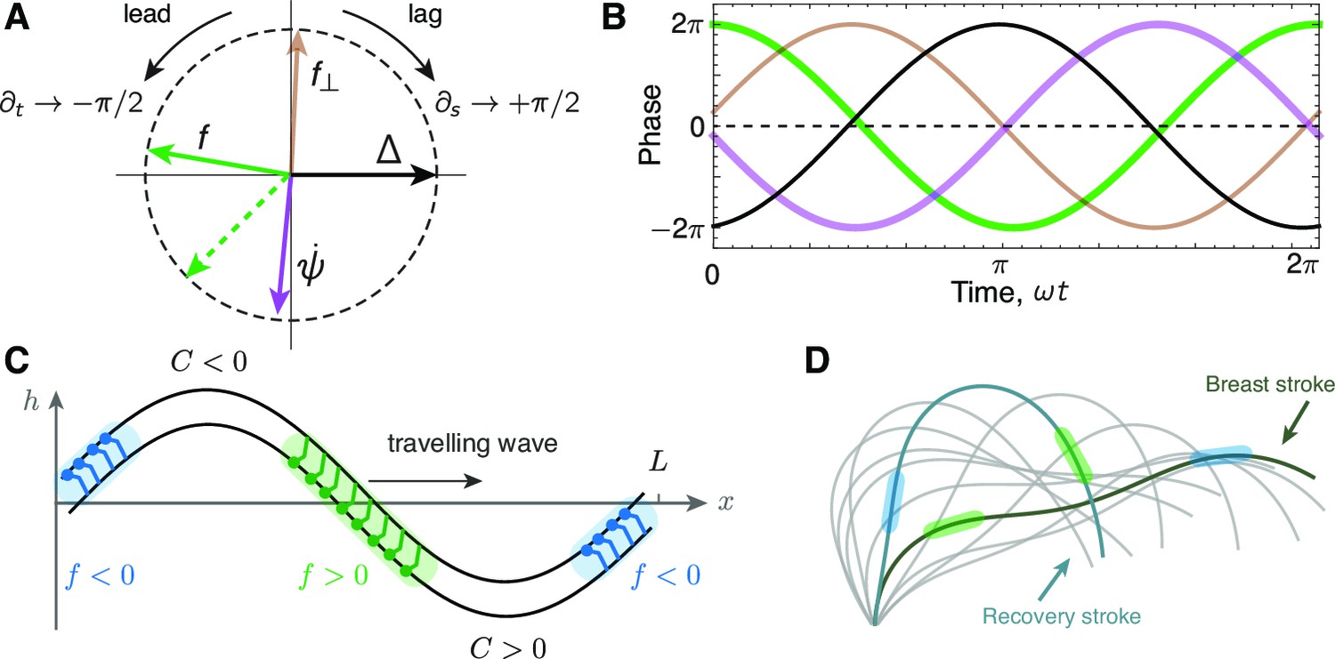
Phase delays and active force distribution on the axoneme.
(A) Polar representation of the phases of sliding , curvature , normal force and the sliding force for a beating axoneme regulated by curvature. For a plane wave, , a time derivative rotates the phase counter-clockwise through radians, while a spatial derivative rotates the phase clockwise by radians. Deviations from the compass points (E, S, W, N) are due to deviations of the axonemal beat from a plane wave. Machin’s prediction for an optimum flagellum is shown as the red dashed line. (B) Time evolution of the quantities in A.(C) Illustration of the local sliding force for a shape of a symmetrically beating axoneme (e.g. mbo2). The regions of motor activity on the upper and lower filament are highlighted in blue and green respectively. (D) Asymmetrically beating wild type axoneme with two shapes highlighted during the breast and recovery strokes. The arrows represent direction of motion of the axoneme, and the colored patches represent the local sliding force on the respective filaments (see panel C and Figure 1).
Figure 10

Sign convention for motors that step towards the base.
See text for details
Author response image 1
Tables
Table 1
Parameters for beat generation in wild type axonemes.
| Sliding control | Curvature control | Normal-force control | ||
|---|---|---|---|---|
| Coefficient of determination | ||||
| Sliding coefficient | ||||
| Curvature coefficient | 0 | 0 | ||
| Normal-force coefficient | 0 | 0 | ||
| Basal impedance | ||||
| Basal sliding (0th mode) | ||||
| Basal sliding (1st mode) |
-
The values reported are mean and standard deviation calculated from axonemes. The average static curvature is , the length , and the frequency rad/s (68 Hz). Note that, for curvature controlled beats, using the value of and an estimate curvature of results in a sliding force of . Since the motor density of an active half of the axoneme is the individual motor force is . For the case of normal force control, the sliding force generated by the motors is of the order of the normal force that they experience, since .
Table 2
Parameters for beat generation in mbo2 mutant axonemes.
| Sliding control | Curvature control | Normal-force control | ||
|---|---|---|---|---|
| Coefficient of determination | ||||
| Sliding coefficient | ||||
| Curvature coefficient | 0 | 0 | ||
| Normal-force coefficient | 0 | 0 | ||
| Basal impedance | ||||
| Basal sliding (0th mode) | ||||
| Basal sliding (1st mode) |
-
Values are averages and standard deviations for axonemes. The static curvature was , the length , and the frequency rad/s, (28 Hz). Note that the values of in normal force control are very spread out and compared to the wild type fits. In fact, in one case we obtained , indicating that motors must amplify the normal force they sense by almost two orders of magnitude. The values for curvature control are very similar to those of wild type fits..
Download links
A two-part list of links to download the article, or parts of the article, in various formats.
Downloads (link to download the article as PDF)
Open citations (links to open the citations from this article in various online reference manager services)
Cite this article (links to download the citations from this article in formats compatible with various reference manager tools)
Dynamic curvature regulation accounts for the symmetric and asymmetric beats of Chlamydomonas flagella
eLife 5:e13258.
https://doi.org/10.7554/eLife.13258


