High-throughput mathematical analysis identifies Turing networks for patterning with equally diffusing signals
- Friedrich Miescher Laboratory of the Max Planck Society, Germany
- The Barcelona Institute of Science and Technology, Spain
- Universitat Pompeu Fabra, Spain
- Institucio Catalana de Recerca i Estudis Avançats, Spain
Figures
Figure 1 with 4 supplements
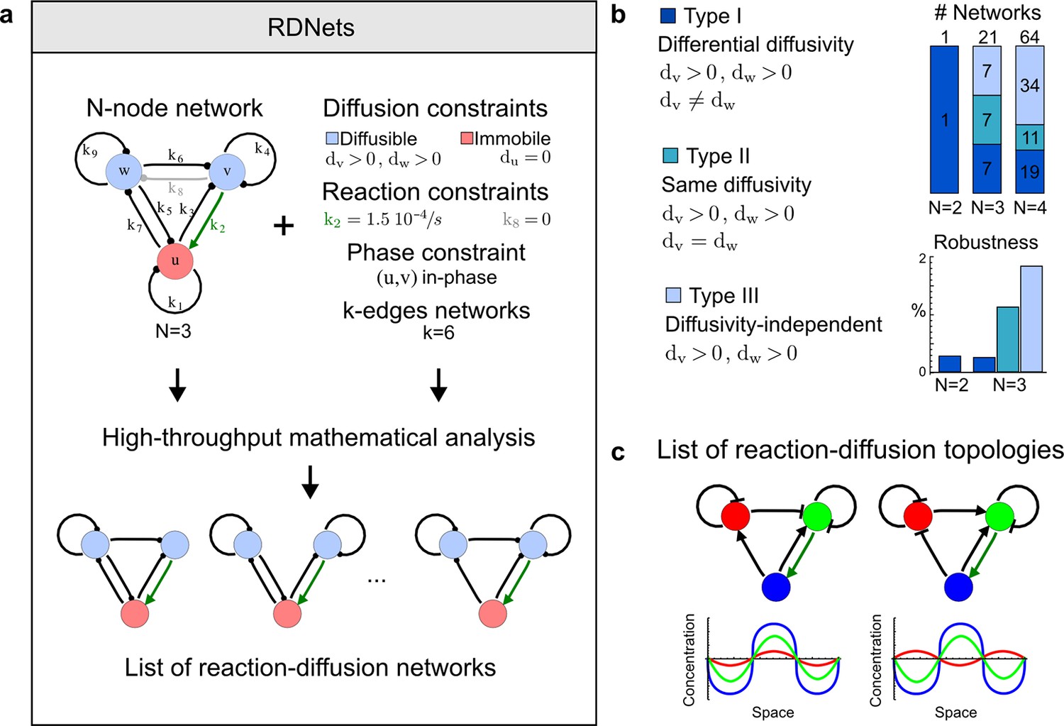
High-throughput screen for reaction-diffusion patterning networks using RDNets.
(a) Schematic representation of the software RDNets to identify pattern-forming networks. RDNets exploits a computer algebra system for high-throughput mathematical analysis of reaction-diffusion networks with N nodes and k edges. Diffusion and reaction constraints, including the number of diffusible (blue) and non-diffusible (red) nodes and quantitative parameters (here: k2, k8), can be specified as inputs. Additionally, the phase of the resulting periodic pattern can be selected. A list of reaction-diffusion networks is given as output. (b) Bar charts summarizing the number of networks for the 2-, 3-, and 4-node signaling network cases. Resulting networks can be of three types: Type I requires differential diffusivity, Type II allows for equal diffusivity, and Type III is diffusivity-independent. Type II and Type III networks are more robust to parameter changes than Type I networks. (c) Simulations of the possible topologies associated with a given network show that the minimal three-node systems can form in-phase and out-of-phase periodic patterns depending on the network topology. See Appendix 6 for a full list of parameters.
Figure 1—figure supplement 1
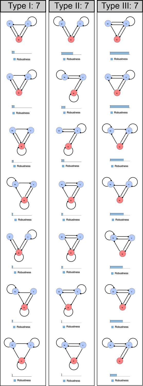
Catalog of all 3-node networks with two diffusible nodes (blue), one non-diffusible node (red) and six interactions.
The relative robustness is shown below each network. Note the higher robustness of Type III networks.
Figure 1—figure supplement 2

Comprehensive catalog of 4-node Type I reaction-diffusion networks with two diffusible (blue) and two non-diffusible (red) nodes representing the interaction between two signaling pathways.
https://doi.org/10.7554/eLife.14022.005
Figure 1—figure supplement 3
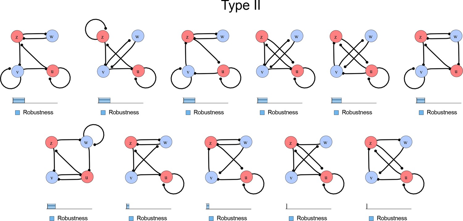
Comprehensive catalog of 4-node Type II reaction-diffusion networks with two diffusible (blue) and two non-diffusible (red) nodes representing the interaction between two signaling pathways.
https://doi.org/10.7554/eLife.14022.006
Figure 1—figure supplement 4
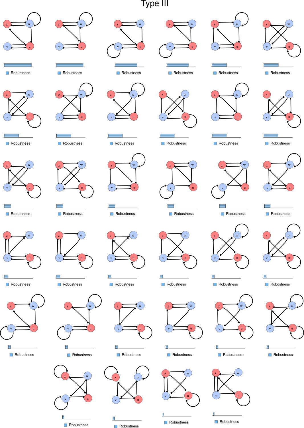
Comprehensive catalog of 4-node Type III reaction-diffusion networks with two diffusible (blue) and two non-diffusible (red) nodes representing the interaction between two signaling pathways.
https://doi.org/10.7554/eLife.14022.007
Figure 2
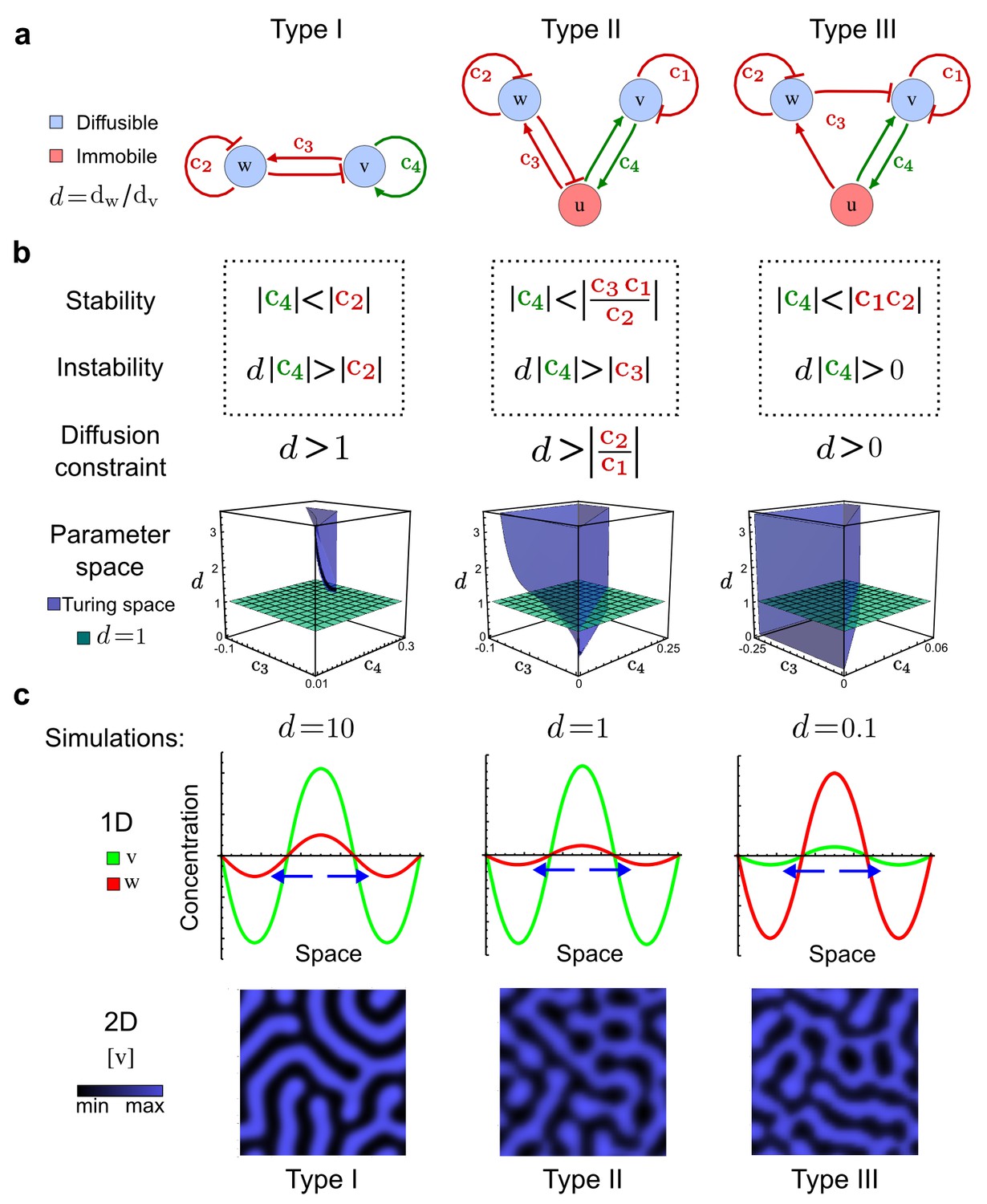
Analysis of the organizing principles underlying reaction-diffusion networks.
(a) Schematic diagram of a 2-node network of Type I, a 3-node network of Type II, and a 3-node network of Type III. c1 to c4 indicate feedback cycles, red indicates overall inhibition and green overall activation, and d=dw/dv represents the diffusion ratio. The two-node network (left column) is a classical activator-inhibitor system, the other two networks are more realistic 3-node networks wired through a cell-autonomous factor u. (b) Linear stability analysis of the topologies shown in (a) reveals that pattern-forming conditions require a trade-off between stability and instability feedback cycles, which gives rise to the diffusion constraint. The blue volume highlights the parameter set that allows for pattern formation (Turing space); the three parameters c3, c4, and d vary independently along the axes. Intersecting the Turing space with a plane of equal diffusion coefficients d=1 shows that, in contrast to Type II and Type III networks, patterning in Type I networks is not possible with equal diffusivities. (c) 1D simulations show that the apparent longer inhibitor range (blue arrows) observed in the Type I network is also maintained in the Type II network even with d=1 and therefore does not result from differential diffusivity. The Type III network with d=0.1 surprisingly shows an apparent longer range for the activator v. 1D and 2D simulations show that Type II and Type III topologies form patterns similar to those generated by classical 2-node models. See Appendix 6 for a full list of parameters.
Figure 3 with 1 supplement
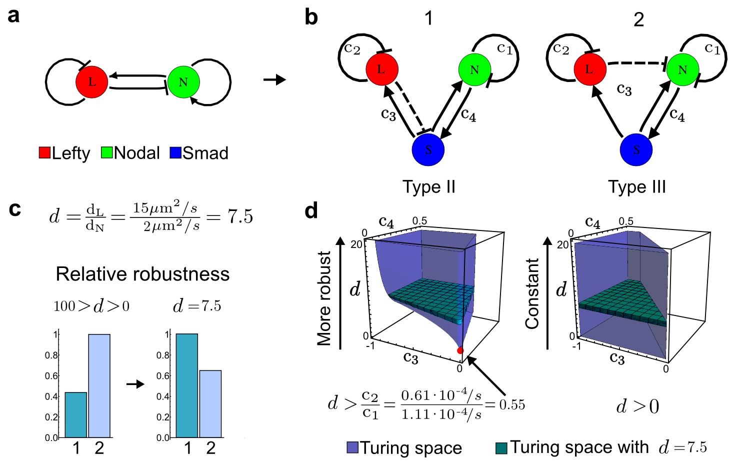
Modeling of the Nodal/Lefty reaction-diffusion system with realistic signaling networks.
(a) Schematic diagram of the Nodal/Lefty activator-inhibitor system. Nodal (green) is the self-enhancing activator that promotes the feedback inhibitor Lefty (red). (b) Extension of the Nodal/Lefty system with an immobile cell/receptor-complex node (blue) to distinguish between two possible feedback modes. In both networks, the self-enhancing activation and the Nodal-induced Lefty expression occurs through a non-diffusible cell/receptor-complex represented by the activated signal transducer pSmad2/3 (S, blue). In the Type II network, Lefty inhibits Nodal through the receptor node S, whereas in the Type III network, Lefty inhibits Nodal directly (dashed lines). (c,d) The Type III network is more robust to parameter changes over a broader range of diffusivities (bar chart on the left and bigger Turing space [blue volume]) compared to the Type II network. However, constraining the two topologies with previously measured diffusion coefficients (d=7.5) demonstrates that the Type II network is more robust for biologically relevant parameters (bar chart on the right and bigger area of the green plane corresponding to d=7.5 within the Turing space [blue volume]). Experimental data for the previously measured clearance rate constants (c1, c2) of Nodal and Lefty predicts that the minimum allowed diffusion ratio for the Type II network is d=0.55 (red dot).
Figure 3—figure supplement 1
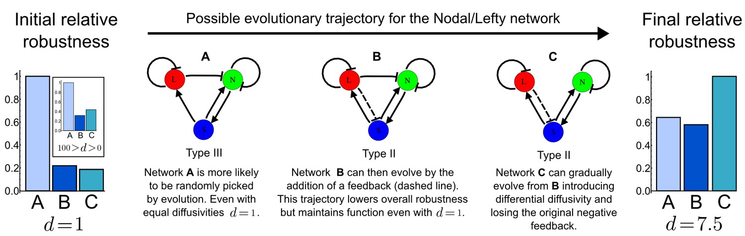
A possible evolutionary scenario for evolving the differential diffusivity of Nodal and Lefty.
Network A (Type III) is more likely to evolve de novo with an initial equal diffusivity (d=1) and for a wider range of diffusion ratios (100>d>0). During evolution, if the negative feedback on Nodal signaling changes (dashed line), network C (Type II) together with differential diffusivity can be selected to increase robustness and therefore fitness.
Figure 4
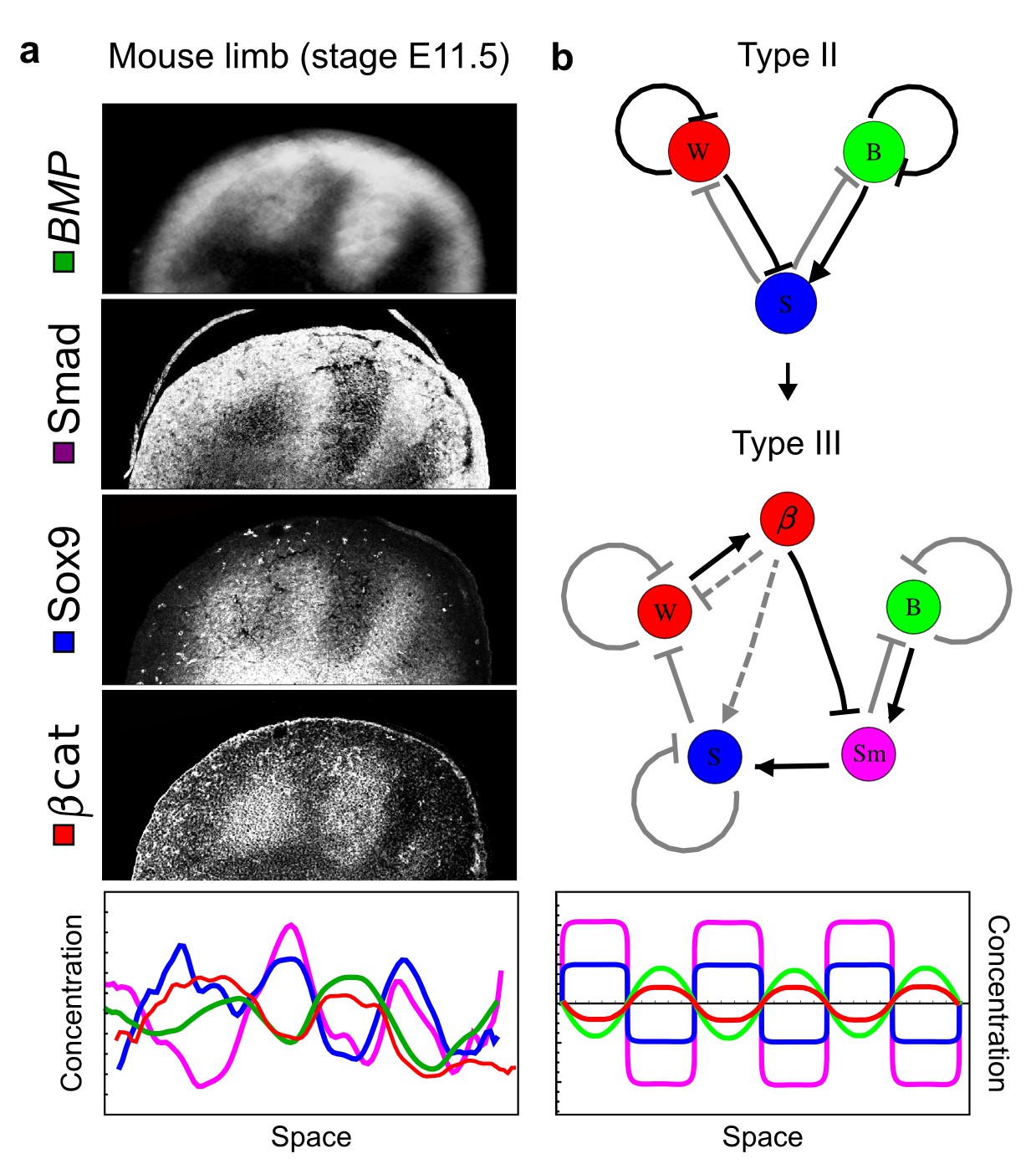
Modeling of mouse digit patterning with realistic signaling networks.
(a) Experimental patterns of BMP (green), pSmad1/5/8 (purple), Sox9 (blue), and β-catenin (red) in a mouse limb at stage E11.5 (data reproduced from Raspopovic et al., 2014). (b) Extension of a previously proposed simple three-node network for digit patterning involving BMP, Sox9, and Wnt to a more realistic five-node network incorporating known interactions (black) between Wnt (W, red), BMP (B, green), Smad1/5/8 (Sm, pink), Sox9 (S, blue), and β-catenin (β, red); interactions predicted by RDNets are shown in gray, and dashed lines correspond to alternative interactions that implement networks with similar robustness. The simulations of the new five-node network recapitulate the unintuitive out-of-phase pattern between BMP expression (green) and its own signaling through pSmad1/5/8 (purple). The mathematical analysis predicts that these patterns can be formed when β-catenin inhibits Sox9 indirectly through pSmad1/5/8. See Appendix 6 for a full list of parameters.
Figure 5 with 1 supplement
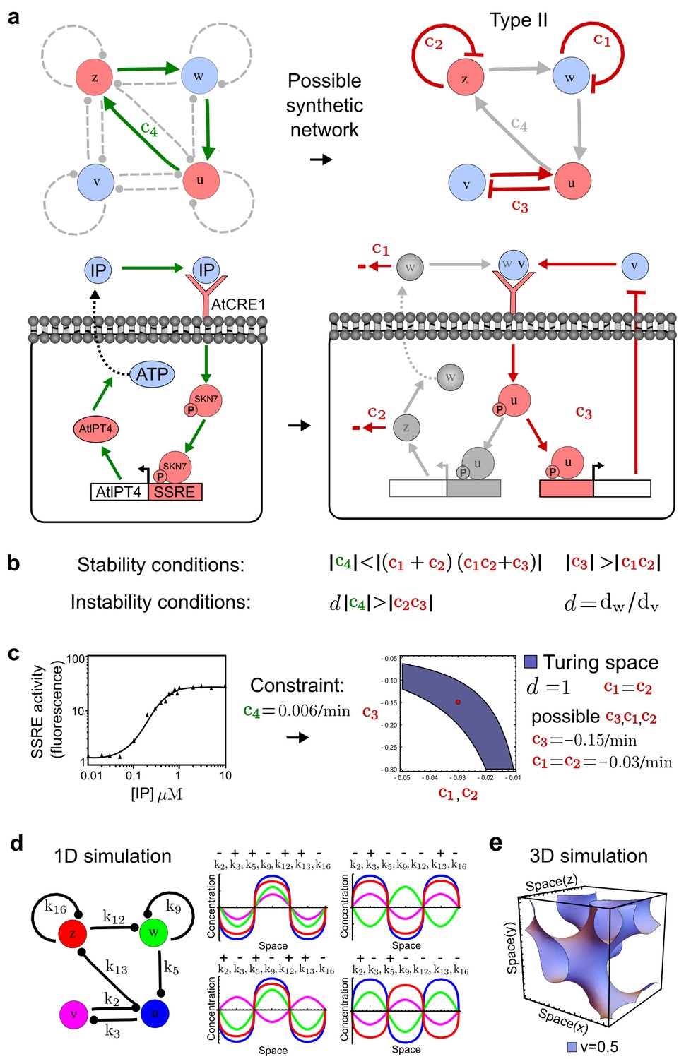
Combining signaling modules to form new synthetic reaction-diffusion networks.
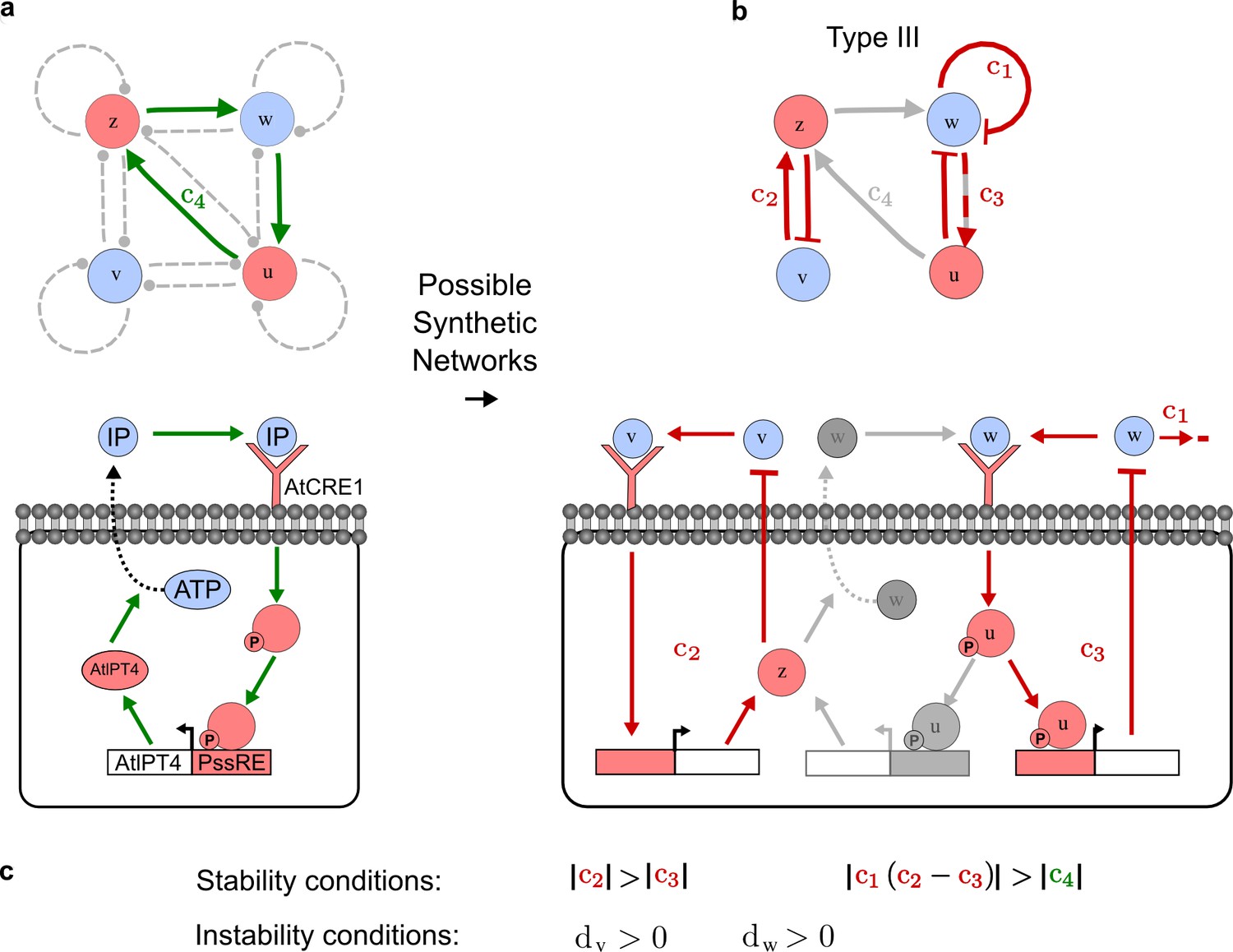
(a) Left: Schematic diagram of a four-node network to engineer a patterning system from an existing signaling module (Chen and Weiss, 2005) that implements a positive feedback (c4, green). In the previously engineered synthetic network, the positive feedback highlighted by c4 was implemented by the hormone Cytokinin isopentenyladenine (IP) that activates the receptor AtCRE1 to induce the SSRE-promoter-driven expression of AtIPT4, which catalyzes IP production. Right: A possible Type II reaction-diffusion network predicted by RDNets, in which the positive feedback module composed of w, u and z (representing IP, receptors/transducers, and AtIPT4 shown in (a)) is extended by a node v that activates u, which in turn inhibits v (cycle c3). The cycles c1 and c2 correspond to signal decay. (b) Stability and instability conditions of the predicted network. (c) Constraining RDNets with previous measurements of the positive feedback cycle c4 obtained by fitting experimental data (graph on the left, Chen and Weiss, 2005) identifies exact parameter ranges for the new interactions in the synthetic reaction-diffusion network (graph and formulae on the right). (d) 1D simulations show that different topologies of this synthetic network can be engineered to produce all possible in- and out-of-phase periodic patterns depending on the sign of the reaction rates shown above the graphs. (e) A 3D simulation of the synthetic patterning system forms tubular structures that could be exploited for tissue engineering.
Figure 5—figure supplement 1
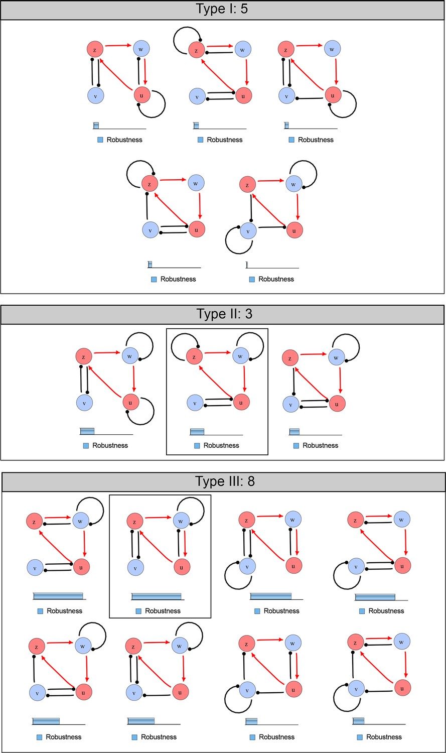
Catalog of possible synthetic networks that extend an existing feedback loop (red arrows).
Networks have 2 diffusible nodes (blue), 2 non-diffusible nodes (red) and seven interactions. The relative robustness is shown below each network. Note the higher robustness of Type III networks. The two boxed circuits correspond to the networks presented in Figure 5 (Type II) and Appendix 4—figure 1 (Type III).
Appendix 1—figure 1
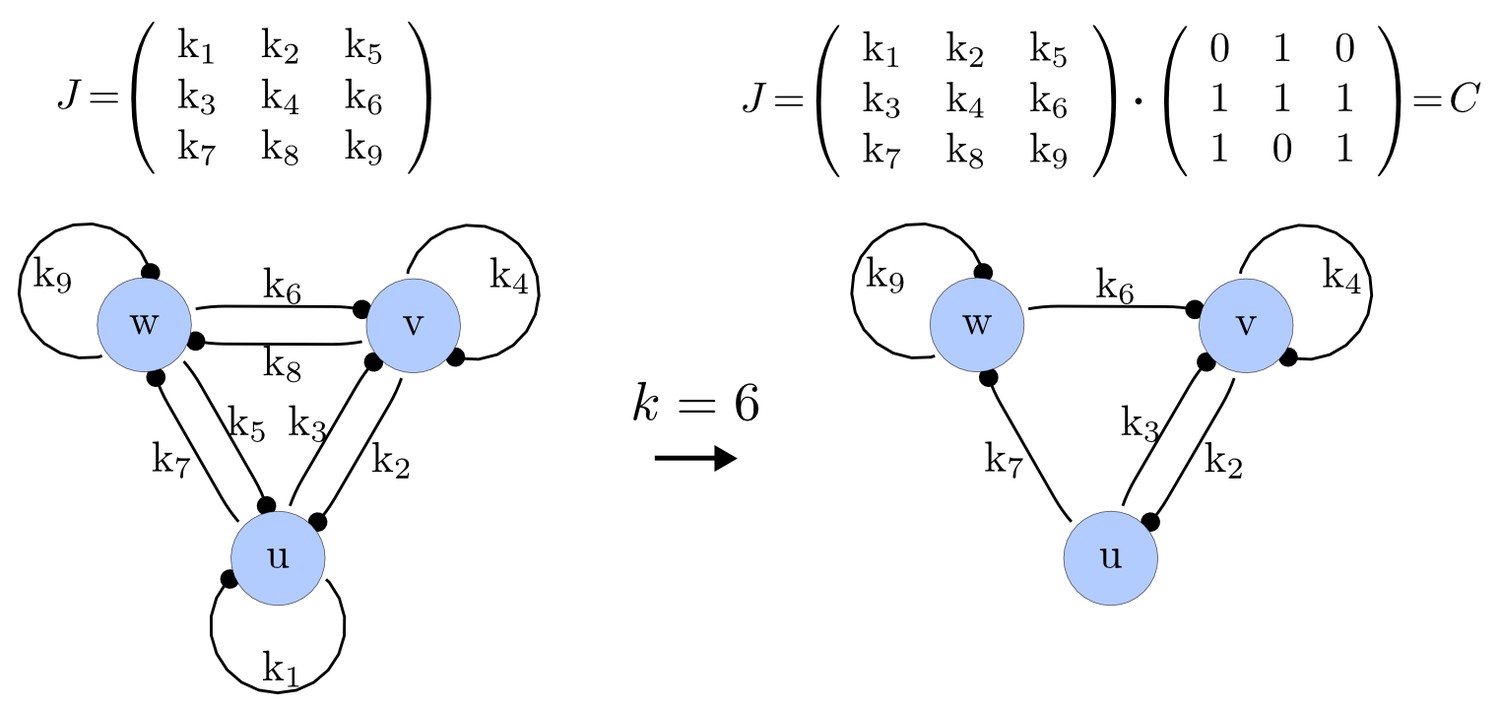
Example of a matrix C and its corresponding network for N = 3 and k = 6.
https://doi.org/10.7554/eLife.14022.015
Appendix 1—figure 2
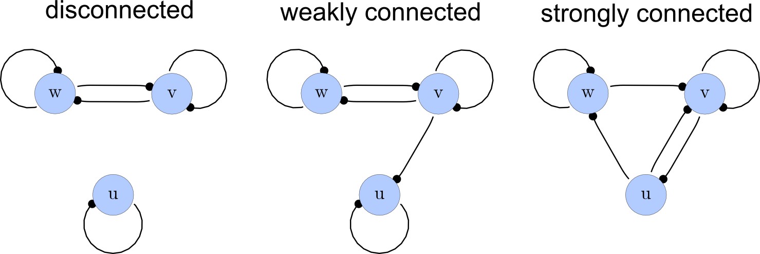
Network connections.
Left: A disconnected network. Middle: A weakly connected network with a read-out node u. Right: A strongly connected network.
Appendix 1—figure 3
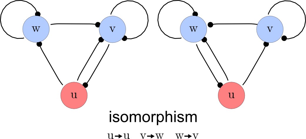
Deleting symmetric networks.
Two symmetric networks with a corresponding isomorphism that maps equivalent nodes are shown.
Appendix 1—figure 4
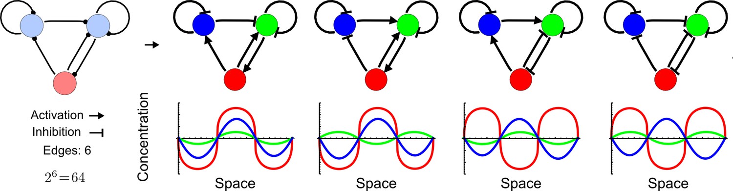
Network topologies determine all possible in- and out-of-phase periodic patterns.
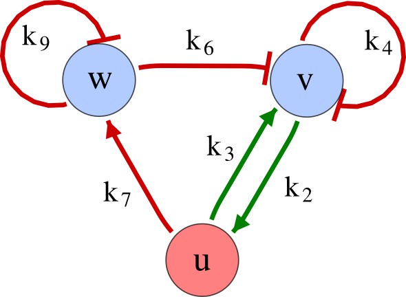
The shown 3-node network with two diffusible (blue) nodes and one non-diffusible (red) node has 6 edges and therefore 26 = 64 topologies. Four of the 64 possible topologies are reaction-diffusion systems and represent all possible in-phase and out-of-phase pattern between the nodes.
Appendix 2—figure 1
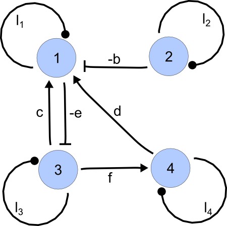
Interaction graph associated with matrix A.
https://doi.org/10.7554/eLife.14022.020
Appendix 2—figure 2
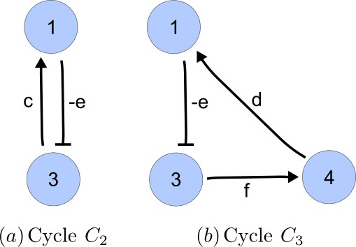
Cycles of length in .
https://doi.org/10.7554/eLife.14022.021
Appendix 2—figure 3
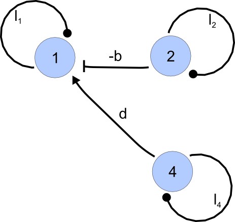
I-subgraph induced by A(γ3).
https://doi.org/10.7554/eLife.14022.022
Appendix 2—figure 4
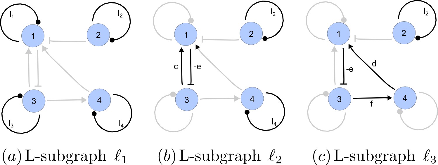
Linear spanning subgraphs of GR[A].
https://doi.org/10.7554/eLife.14022.023
Appendix 2—figure 5

Output from RDNets showing the full set of conditions required for pattern formation in the Type I network shown in Figure 2, left panel.
The trade-off between stabilizing and destabilizing feedbacks that underlies the minimum diffusion ratio d is highlighted with orange boxes.
Appendix 2—figure 6
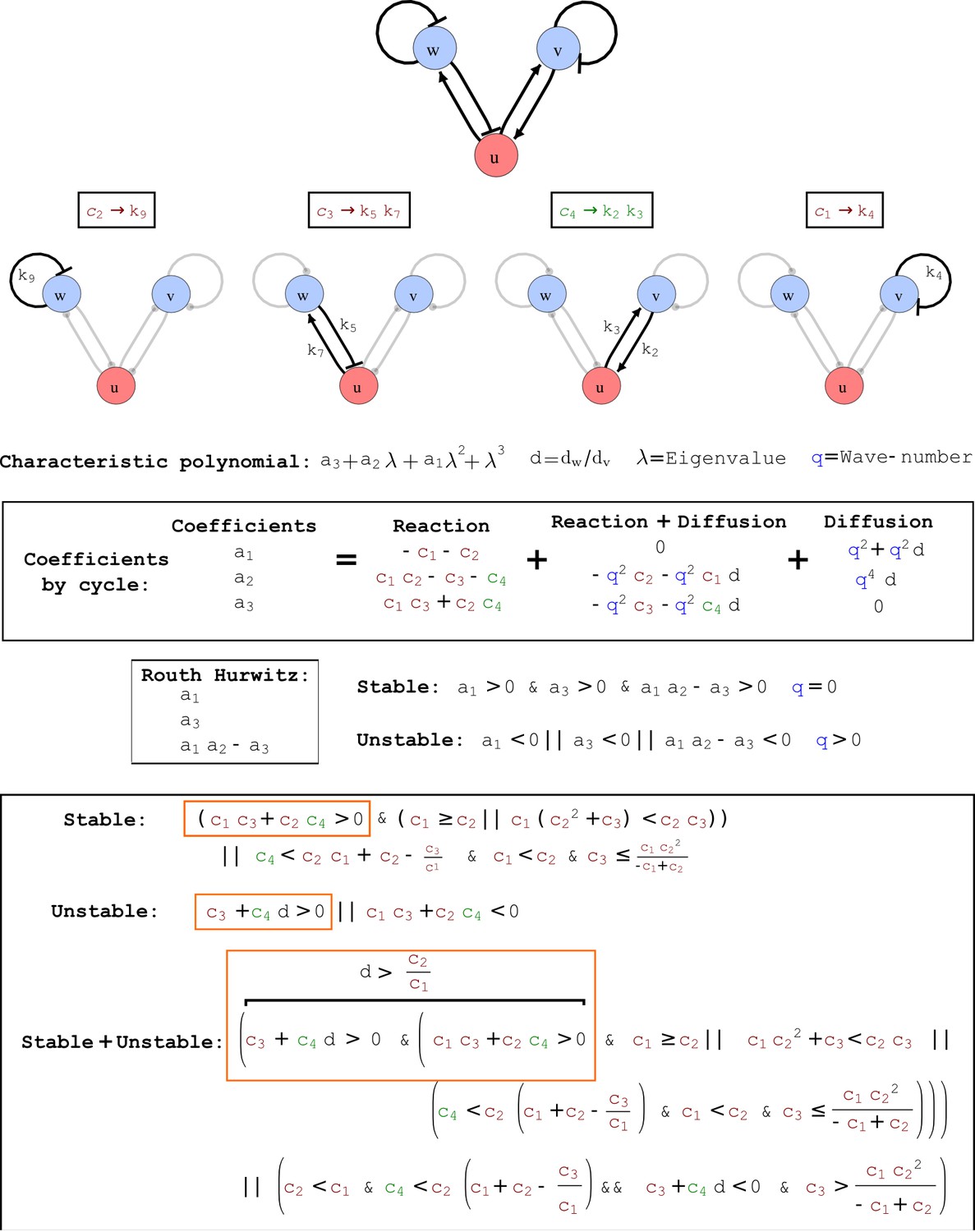
Output from RDNets showing the full set of conditions required for pattern formation in the Type II network shown in Figure 2, middle panel.
The trade-off between stabilizing and destabilizing feedbacks that underlies the minimum diffusion ratio d is highlighted with orange boxes.
Appendix 2—figure 7
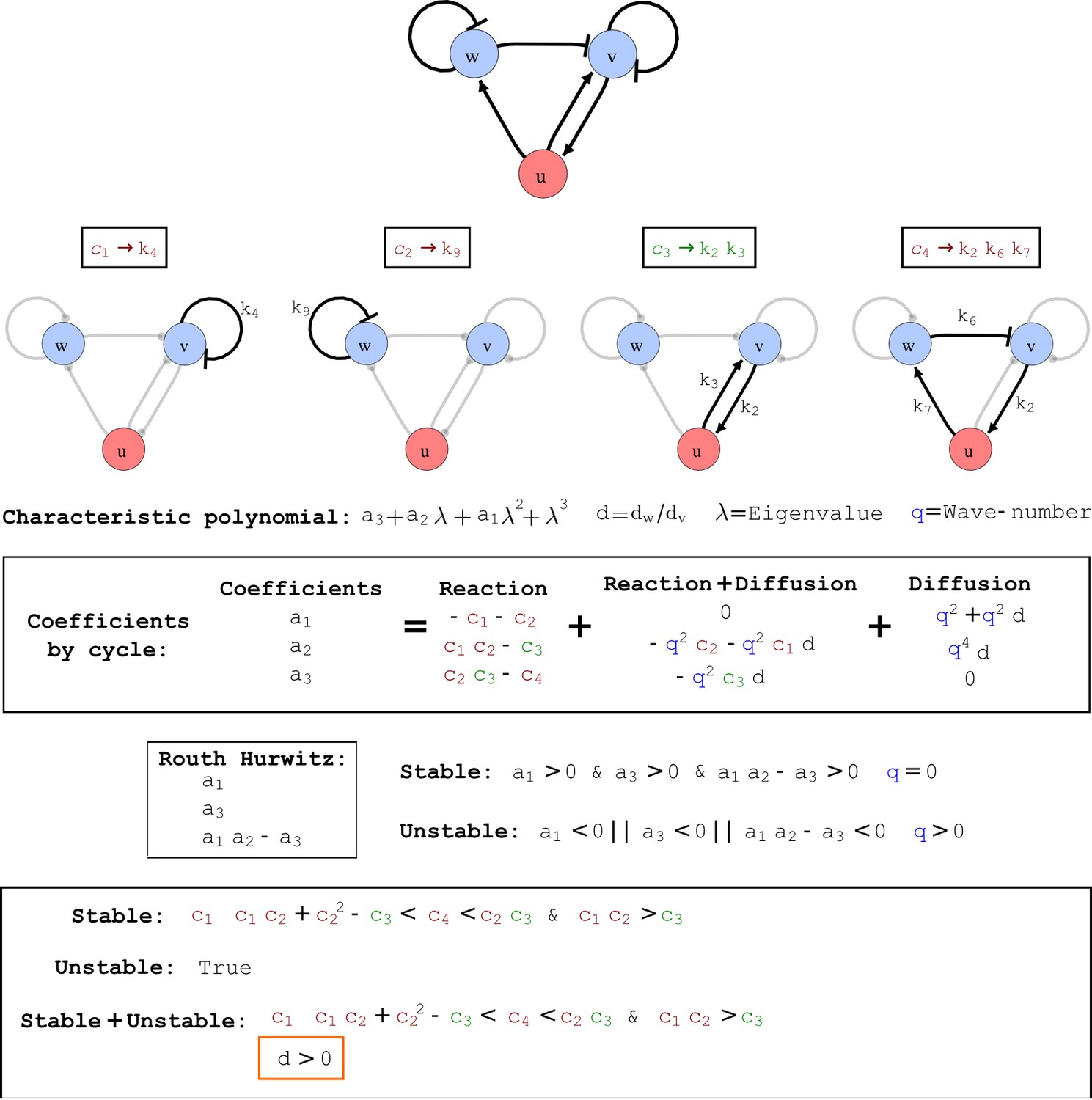
Output from RDNets showing the full set of conditions required for pattern formation in the Type III network shown in Figure 2, right panel.
The trade-off between stabilizing and destabilizing feedbacks that underlies the minimum diffusion ratio d is highlighted with orange boxes.
Appendix 3—figure 1
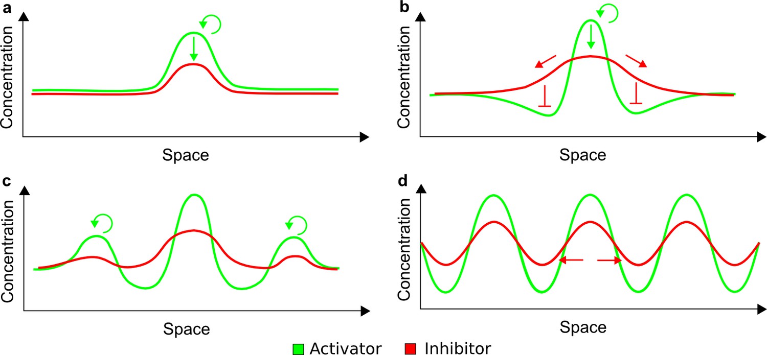
Schematic representation of the activator-inhibitor model based on LALI.
(a) Small random fluctuations in the homogeneous distribution of the activator and the inhibitor give a little advantage to the activator to promote itself and to grow in concentration (green arrows). Since the activator promotes the inhibitor, a higher concentration of the inhibitor is also formed in the same region. (b) The inhibitor diffuses more rapidly than the activator and thereby inhibits the formation of other activator peaks in surrounding regions. It also promotes further growth of the activator due to the local decrease of the inhibitor. (c) Other activation peaks are formed by the same mechanism. (d) The overall process leads to the formation of periodic patterns, where the different spatial profiles of activator and inhibitor peaks are assumed to reflect the higher diffusivity of the inhibitor (red arrows).
Appendix 3—figure 2
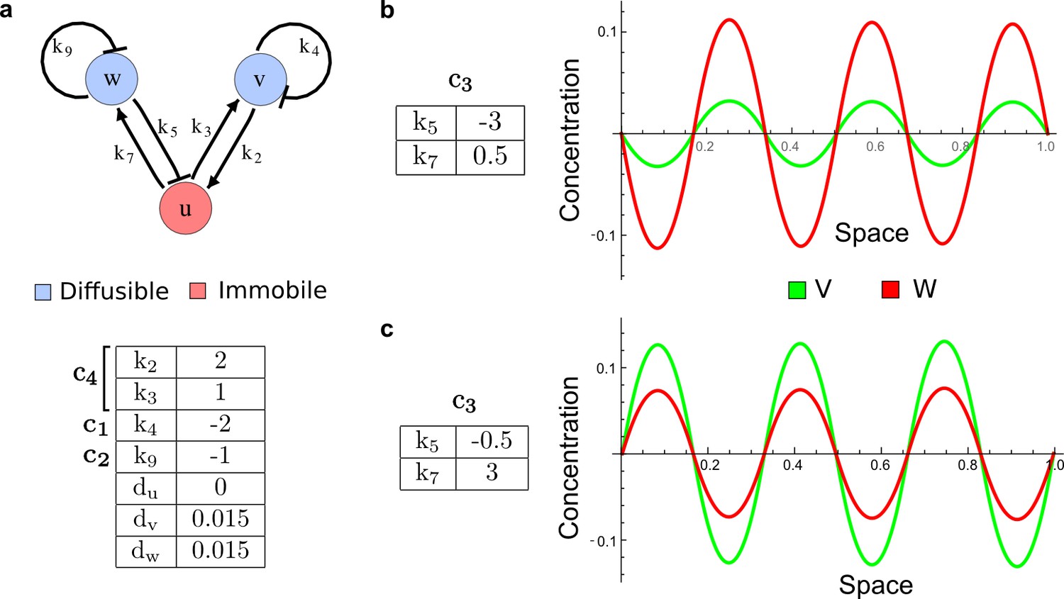
Different ranges of the pattern of v and w in the network of Figure 2c.
(a) The Type II network shown in Figure 2c (center) with reaction rates that implement the cycles c1, c2, c4 and diffusion rates. (b–c) Different reaction rates for the cycle c3 determine different ranges for the peaks of v and w despite their identical diffusion coefficients and half-lives.
Appendix 3—figure 3
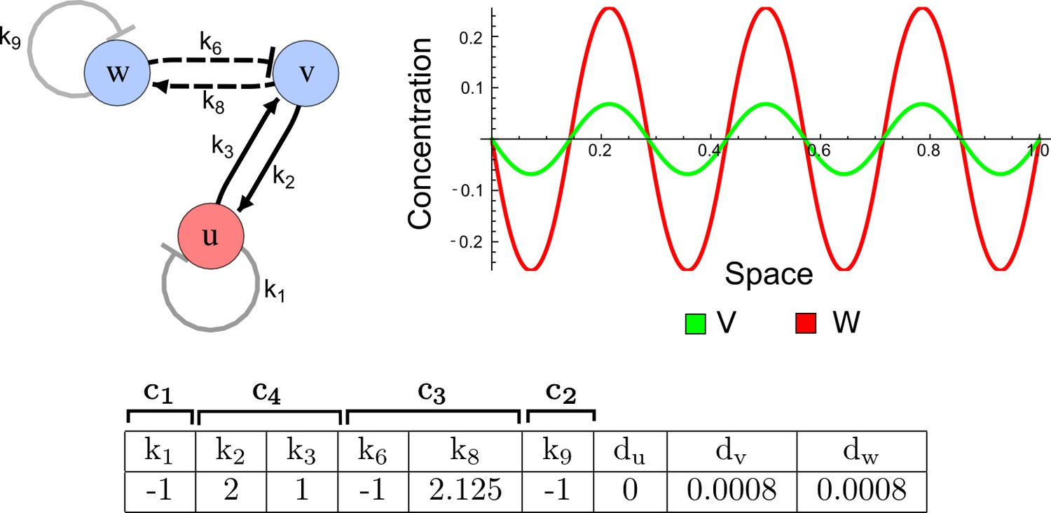
Opposite pattern between the activator-inhibitor model and a Type II network.
On the left: In the three-node network, the non-diffusible node u and the diffusible node v fulfill the role of the activator by mutually promoting each other (solid black lines) and by promoting their own inhibitor w (dashed lines). On the right: In contrast to the patterns of a classical two-node activator-inhibitor system, numerical simulations of the three-node network show activator peaks of v that appear more extended than inhibitor peaks of w.
Appendix 3—figure 4
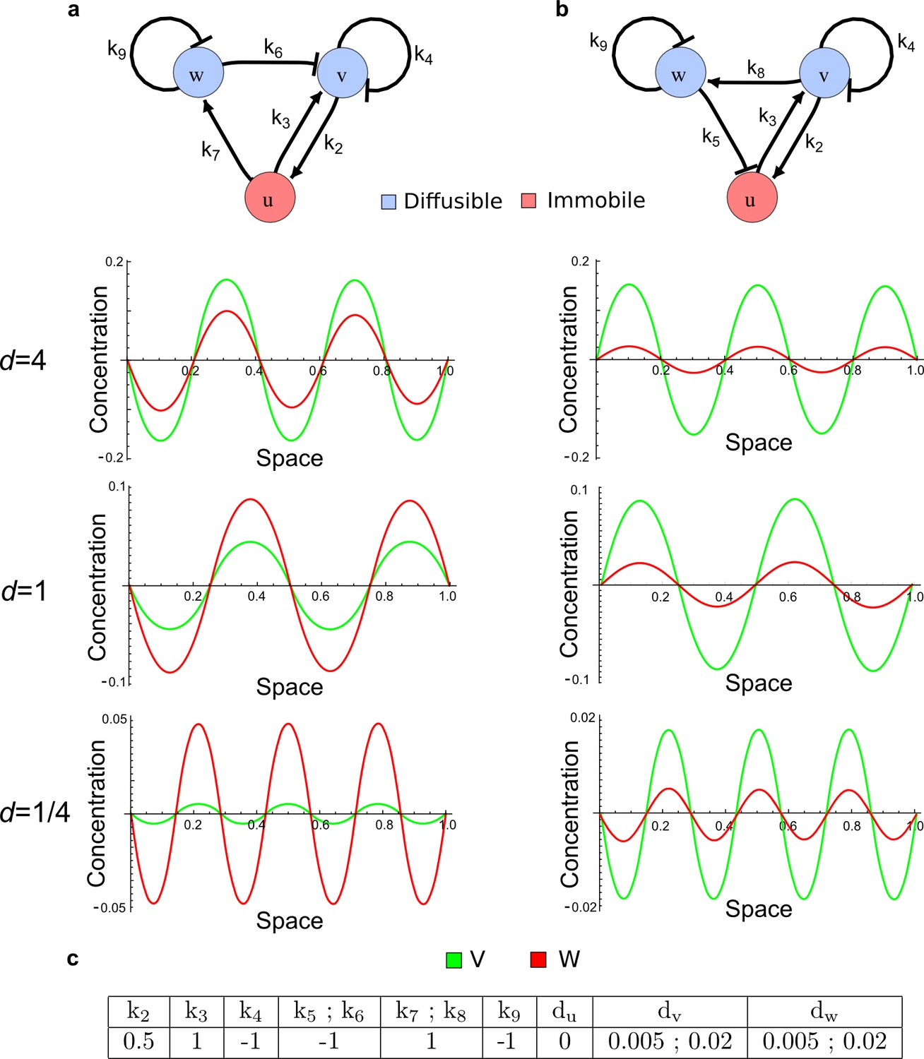
Opposite ranges for the peaks of v and w in Type III networks.
(a) Numerical simulations of the network shown in Figure 2c (right) with different diffusion ratios d: With d = 4, the periodic patterns of v and w are similar to the patterns of an activator and an inhibitor, respectively; but with d = 1 and d = 1/4, opposite patterns are observed. (b) A similar Type III network shows periodic patterns of v and w that are similar to the pattern of classical two-component activator-inhibitor systems independently of the diffusion ratio d. (c) Parameters used for the simulations in a and b. Identical parameters were used for the rates k5;k6 and k7;k8. The diffusion coefficients were set to dv = 0.005 and to dw = 0.02 for the case with d = 4, to dv = 0.02 and dw = 0.02 for the case with d = 1, and to dv = 0.02 and dw = 0.005 for the case with d =1/4.
Appendix 3—figure 5
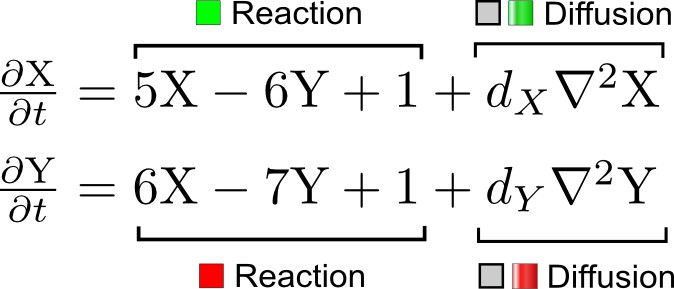
A simple system of two reaction-diffusion equations proposed by Turing.
X corresponds to the activator and Y to the inhibitor in the activator-inhibitor model.
Appendix 3—figure 6
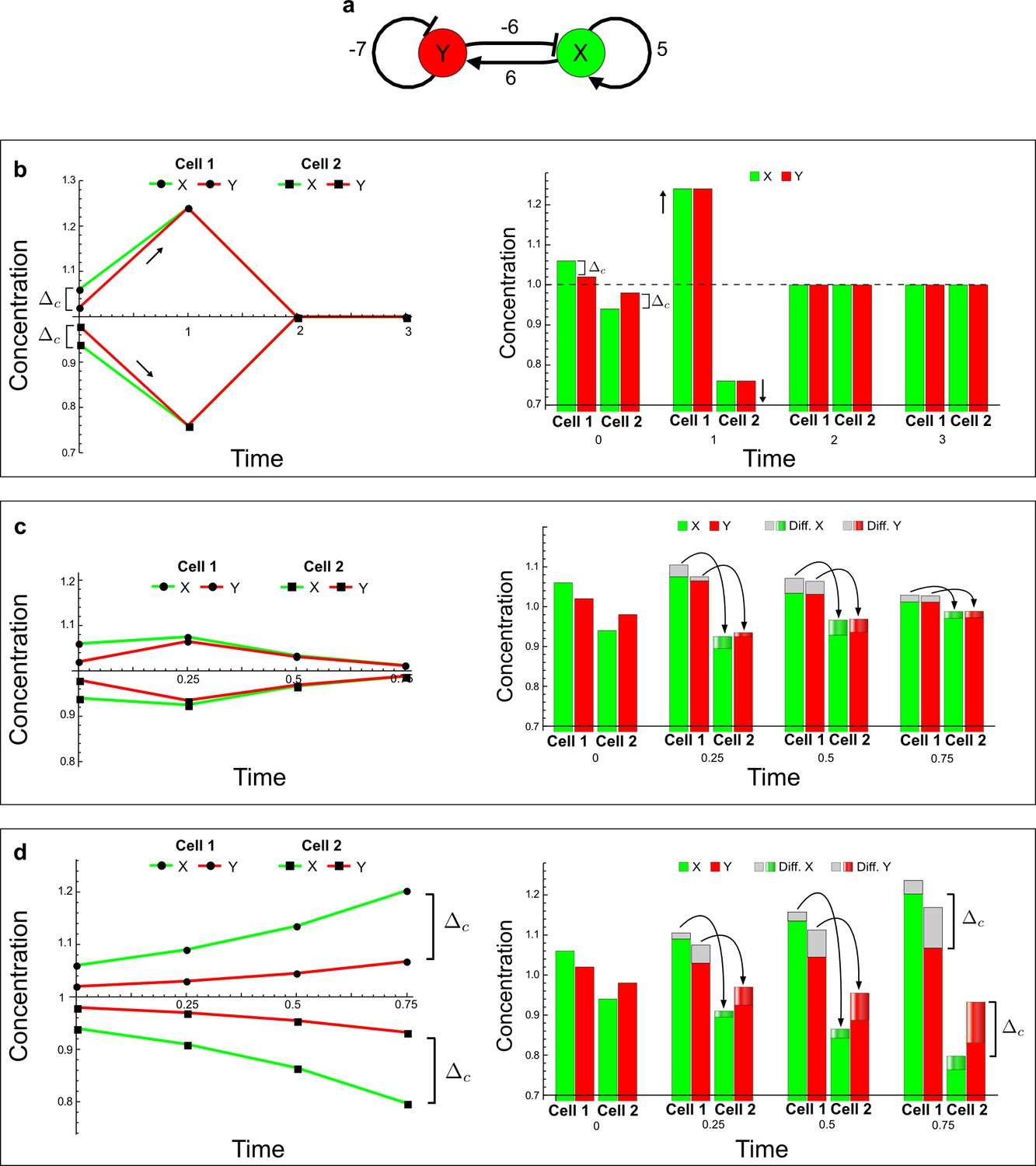
The original example proposed by Turing to show how diffusion can destabilize a reaction-diffusion system by amplifying small fluctuations.
(a) The network diagram of the simple example proposed by Turing: X corresponds to the activator and Y to the inhibitor in the LALI activator-inhibitor model. (b–d) Numerical simulations on a pair of cells (cell 1 and cell 2) with initial conditions X = 1.06,Y = 1.02 in the first cell and X = 0.94,Y = 0.98 in the second cell as originally proposed by Turing. On the left, a graph shows the concentration change of X (green line) and Y (red line) over time in both cells. On the right, the histograms show the same concentration changes over time but additionally highlight the change due to diffusion: gray regions correspond to the amount of X and Y that diffuses out from the first cell and diffuses into the second cell as shown by graded green and red regions for X and Y, respectively. The diffusion process is represented by black arrows. (b) No diffusion: When X and Y do not diffuse, the system goes back to the equilibrium state X = 1, Y = 1 (dashed line). However, the small difference Δc between X and Y in the initial conditions stimulates the system to transiently deviate above and below the equilibrium state (black arrows) in the first and second cell, respectively (see the concentration at time 1). The intrinsic stability of the system eventually guarantees that Δc is reduced over time (see equations in Appendix 3—figure 5), and equal amounts of X and Y in the same cell bring the system back to equilibrium. (c) Equal diffusion: When X and Y diffuse equally, the system quickly returns to equilibrium. Diffusion acts as an equilibrating force by redistributing more activator than inhibitor due to the higher concentration difference of activator between cell 1 and cell 2 (see the larger flow of the activator with respect to the inhibitor at time 0.25 and 0.5). (d) Differential diffusivity: If the inhibitor Y diffuses faster than X, the larger flow of Y maintains the relative difference Δc between activator and inhibitor in both cells and the systems keeps deviating from equilibrium. In cell 1, the greater dilution of the inhibitor with respect to the activator allows the activator and the inhibitor to grow further. In cell 2, the larger amount of inhibitor allows the activator and the inhibitor to decrease further since the inhibitor inhibits itself as well as the activator.
Appendix 3—figure 7
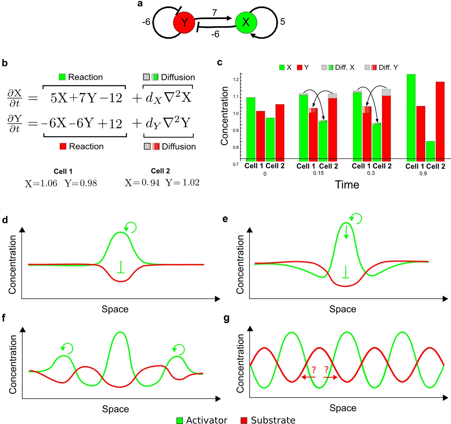
Schematic representation of the substrate-depletion model.
(a) The network diagram of a substrate-depletion model: The activator X (green) inhibits the substrate Y (red) and promotes itself. (b) Equations of the substrate-depletion model and initial conditions used for the simulation in c. A constitutive removal of the activator (−12) and a constitutive production of the substrate (+12) were chosen to have an equilibrium state in X = 1, Y = 1 as in the original example proposed by Turing. (c) Simulation on a pair of cells shows that the greater diffusivity of the substrate Y plays a similar role as in the activator-inhibitor model by simultaneously destabilizing the system in opposite directions. In the first cell, the arrival of more substrate allows the activator to grow further, whereas in the second cell the dilution of the substrate leads to a decrease in activator and consequently to an overall increase of the substrate. Thus, the model simultaneously deviates from equilibrium when the activator X is high and the substrate Y is low and vice versa. (d–g) Schematic representation of an attempt to interpret the substrate-depletion model within the LALI framework based on local auto-activation and lateral inhibition. (d) A local advantage of the activator allows the formation of an activation peak (green) with correspondent depletion of the substrate (red). (e) The peak of activation stops expanding not due to the differential diffusivity but because the substrate falls below a certain threshold. Indeed, it appears that the higher diffusion of the substrate would promote further growth of the activator rather than limit its expansion (red arrows). The role of differential diffusivity is unclear. (f) Other peaks are formed in surrounding regions by the same mechanism. (g) Opposite periodic patterns of the activator and substrate are eventually formed.
Appendix 3—figure 8
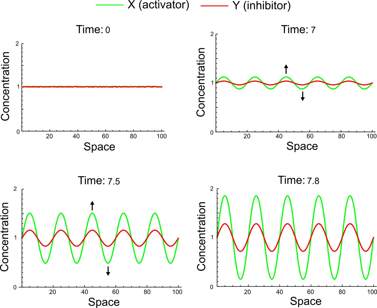
Simulation of the original reaction-diffusion network proposed by Turing started with random perturbations around the homogeneous steady state and uniformly distributed in the interval (-0.001, 0.001).
Black arrows highlight the deviations of the activator (green) and the inhibitor (red). These deviations are simultaneously promoted above and below the steady state across the entire spatial domain by the differential diffusivity. The final aspect of the periodic peaks does not reflect a difference between activation and inhibition ranges but rather reflects a different speed of growth for each periodic pattern, which is determined both by reaction and diffusion terms.
Appendix 3—figure 9
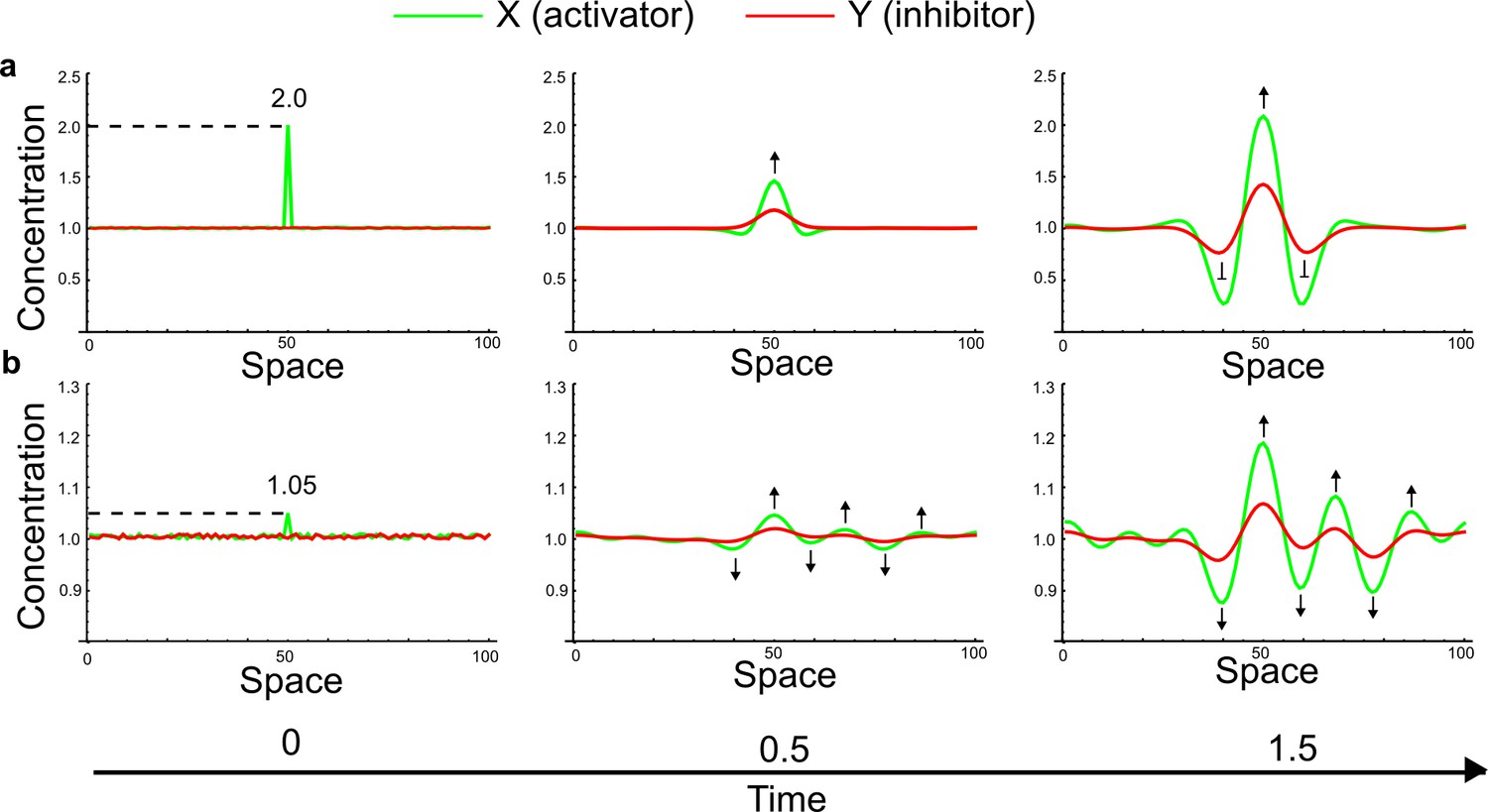
Simulations of the original example proposed by Turing (Appendix 3—figure 5) started with small random fluctuations around the homogeneous steady state and a large localized concentration of activator at the center of the domain.
(a) When the localized perturbation has a high magnitude, after an initial dilution of the perturbation patterning dynamics in agreement with the classical interpretation based on the LALI mechanism can be observed: A peak of activator forms first, and a higher amount of inhibitor appears to diffuse into the surrounding areas to inhibit the spreading of the activator. (b) If the magnitude of the localized perturbation is reduced, a simultaneous formation of activator and inhibitor peaks is observed (black arrows). This suggests that LALI is only a phenomenological description of the effect of the large localized perturbation of the activator rather than a bona fide model of the dynamics of real patterning systems.
Appendix 3—figure 10
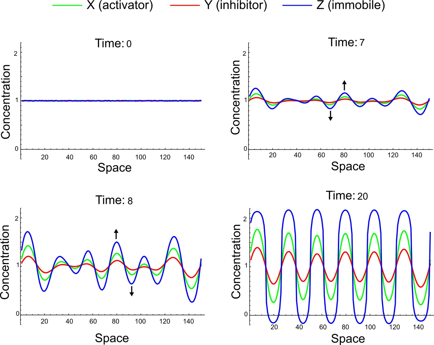
A simulation of the three-component reaction-diffusion system (Equation 32) with dX = dY = 1, dZ = 0 initialized with random perturbations around the homogeneous steady state uniformly distributed in the interval (-0.001, 0.001).
X, Y, and Z simultaneously deviate above and below the steady state across the entire spatial domain (black arrows). The final aspect of the periodic peaks does not reflect a difference between the ranges of the activator X and the inhibitor Y, but rather reflects a different speed of growth for each periodic pattern, which is determined both by reaction and diffusion terms.
Appendix 3—figure 11
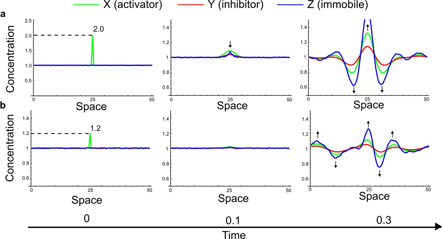
Simulations of the three-node extension to the original example proposed by Turing (Equation 32) started with small random fluctuations around the homogeneous steady state and a large localized concentration of activator at the center of the domain.
(a) Even when the localized perturbation has a high magnitude similar to the simulations in Appendix 3—figure 9, the patterning dynamics are inconsistent with the LALI mechanism since the inhibition does not spread faster into the surrounding areas than the activator. (b) If the magnitude of the localized perturbation is reduced, a simultaneous formation of activator and inhibitor peaks is observed similar to the simulations in Appendix 3—Figure 9 (black arrows).
Appendix 3—figure 12
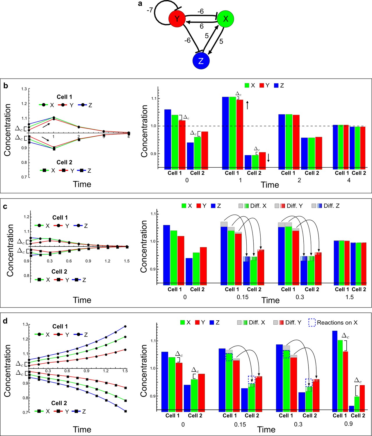
A Type III network that extends the simple example proposed by Turing.
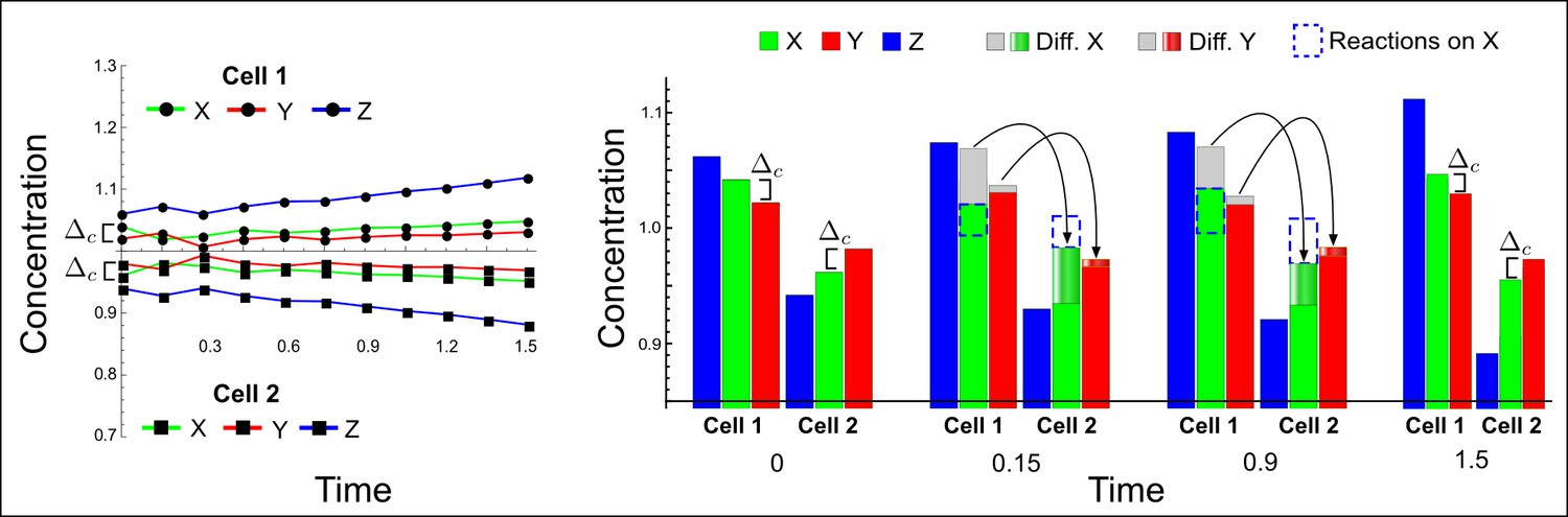
(a) The self-enhancement of the activator X is implemented by a mutual activation with Z, and both X and Z are inhibited by the inhibitor Y. (b–d) Numerical simulations of a pair of cells (cell 1 and cell 2) with initial conditions X = 1.04, Y = 1.02, and Z = 1.06 in the first cell, and X = 0.96, Y = 0.98, and Z = 0.94 in the second cell. On the left, the graphs show the concentration changes of X (green line), Y (red line), and Z (blue line) over time in both cells. On the right, the histograms show the same concentration changes over time but additionally highlight the change due to diffusion: Gray regions correspond to the amount of X, Y, and Z that diffuse out from the first cell, and the amount that diffuses into the second cell is indicated by graded green, red, and blue regions for X, Y, and Z, respectively. The diffusion process is represented by black arrows. (b) No diffusion: When X, Y, and Z do not diffuse, the system returns to the equilibrium state X = 1, Y = 1 and Z = 1 (dashed line). However, the small differences between X, Y, and Z in the initial conditions stimulate the system to transiently deviate above and below the equilibrium state (black arrows) in the first and second cell, respectively (see the concentration at time 1). The intrinsic stability of the system guarantees that Δc is reduced over time, and the system returns to equilibrium. (c) Equal diffusion: When X, Y, and Z diffuse equally, the system also quickly returns to equilibrium. Diffusion acts as an equilibrating force by redistributing more X and Z, and less Y, due to the higher concentration difference of X and Z between cell 1 and cell 2 (see the larger flow of X (green) and Z (blue) with respect to the flow of Y (red) at time 0.15 and 0.3). (d) Equal diffusion of X and Y in the presence of non-diffusible Z: Diffusion still acts as an equilibrating force by redistributing more X than Y from the first to the second cell. However, the fact that Z is not subjected to diffusion in combination with the diffusion of Y allows the reaction term of X (dashed blue line and first equation in Equation (32) to compensate for the larger flow of X. For example, at time 0.15 Z and Y in the first cell promote an increase of X (dashed blue line) that is greater than the amount of X that diffuses out (gray region above the green bar), while Z and Y in the second cell promote a decrease of X (dashed blue line) that is larger than the amount of X that diffuses in (graded green). At the next time point, the dilution of Y allows Z to further diverge from the equilibrium state (see third equation in Equation [32]) and together with Z promotes a stronger compensation (dashed blue line) for the even larger flow of X. In this way, the system increases the difference between X and Y (Δc) despite their equal diffusivities and keeps deviating them from equilibrium in opposite directions.
Appendix 3—figure 13
Numerical simulations of the Type III network shown in Appendix 3—figure 12a with an immobile reactant Z and X diffusing four time faster than Y (dX = 4, dY = 1, dZ =0).
In this case, there is an even larger flow of X from the first to the second cell. Initially, the immobile reactant Z is not able to compensate for this larger flow (see time point 0.15, where the dashed line that represents the reaction term of X is smaller than the diffusion of X [gray and graded green regions]), which allows the activator to decrease below the inhibitor level in the first cell and to increase above the inhibitor level in the second cell. In turn, the deviation from equilibrium of the immobile reactant Z is also slightly reduced (see the blue line at time point 0.3 in the graph on the left). However, since Z is not diluted by diffusion, it can recover and grow further over time because of the diffusion of Y. Z and Y together are able to eventually compensate for the flow of X (see the larger contribution of the reaction term of X at time point 0.9 in the histograms (dashed blue line) with respect to the diffusion of X [gray and graded green regions]). This allows to quickly restore the initial relative difference between X and Y and to keep deviating from equilibrium.
Appendix 4—figure 1
An alternative synthetic network for the case in Figure 5.
(a) A previous synthetic circuit was developed to implement a positive feedback loop between the cytokinin IP and its signaling in yeast. (b) A robust Type III network identified by RDNets as a possible extension with three new negative feedbacks c1, c2, c3 to form a reaction-diffusion pattern. (c) Pattern forming conditions for the network shown in b. Note the extremely simple requirements on cycle strength.
Appendix 5—figure 1
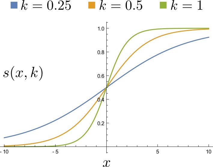
A sigmoid regulation function with different k values.
https://doi.org/10.7554/eLife.14022.041
Appendix 5—figure 2
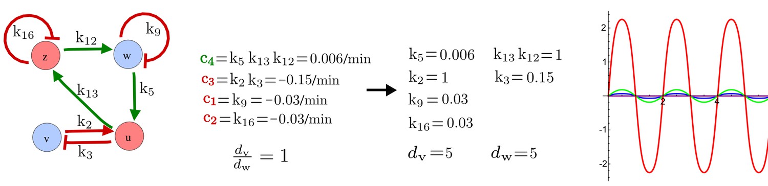
Simulation of the synthetic circuit in Figure 5.
Left: Parameters used in Equation 35 to simulate the synthetic circuits shown in Figure 5. Right: One-dimensional simulation using the sigmoid regulation terms.
Appendix 6—figure 1
Example of a three-node network.
https://doi.org/10.7554/eLife.14022.043
Appendix 6—figure 2

Network for the simulation in Figure 2c, left.
https://doi.org/10.7554/eLife.14022.049
Appendix 6—figure 3

Network for the simulation in Figure 2c, center.
https://doi.org/10.7554/eLife.14022.050
Appendix 6—figure 4

Network for the simulation in Figure 2c, right.
https://doi.org/10.7554/eLife.14022.051
Appendix 6—figure 5

Network for the simulation in Figure 4b.
https://doi.org/10.7554/eLife.14022.052Tables
Table 1
From an initial number of possible networks (Step 1), RDNets progressively identifies reaction-diffusion networks that can form a pattern (Step 6).
| Steps | 3 nodes | 4 nodes | ||
|---|---|---|---|---|
| # networks | # topologies | # networks | # topologies | |
| 1. Minimal systems | 84 | 5376 | 11440 | 1464320 |
| 2. Strongly connected | 48 | 3072 | 2284 | 292352 |
| 3. Non-symmetrical | 25 | 1600 | 597 | 76416 |
| 4. Stable | 24 | 556 | 324 | 8640 |
| 5-6. Reaction-diffusion | 21 | 84 | 64 | 512 |
Appendix 1—Table 1
Minimal network sizes for .
| 2 | 3 | 4 | 5 | |
| minimal | 4 | 6 | 7 | 8 |
Appendix 6—Table 1
Parameters for the simulation in Figure 1c, left.
| 1.5 E-4 | 0.33 E-4 | -1E-4 | -0.67 E-4 | 1 | -1 | 0 | 0.06 | 0.06 |
Appendix 6—Table 2
Parameters for the simulation in Figure 1c, right.
| 1.5 E-4 | 0.33 E-4 | -1E-4 | 0.67 E-4 | -1 | -1 | 0 | 0.06 | 0.06 |
Appendix 6—Table 3
Parameters for the simulation in Figure 2c, left.
| 0.5 | -1 | 0.53125 | -1 | 0.0125 | 0.05 |
Appendix 6—Table 4
Parameters for the simulation in Figure 2c, center.
| 0.125 | 1 | -0.5 | -1 | 0.09375 | -0.25 | 0 | 0.02 | 0.02 |
Appendix 6—Table 5
Parameters for the simulation in Figure 2c, right.
| 0.104 | 1 | -1 | -0.5 | 1 | -0.25 | 0 | 0.1 | 0.01 |
Appendix 6—Table 6
Parameters for the simulation in Figure 4b.
| 0.5 | -1 | 1 | -1 | -1 | -1 | -1 | -1 | 1 | 0 | 0 | 0.05 | 0.05 | 0 |
Download links
A two-part list of links to download the article, or parts of the article, in various formats.
Downloads (link to download the article as PDF)
Open citations (links to open the citations from this article in various online reference manager services)
Cite this article (links to download the citations from this article in formats compatible with various reference manager tools)
High-throughput mathematical analysis identifies Turing networks for patterning with equally diffusing signals
eLife 5:e14022.
https://doi.org/10.7554/eLife.14022


