TissueMiner: A multiscale analysis toolkit to quantify how cellular processes create tissue dynamics
Figures
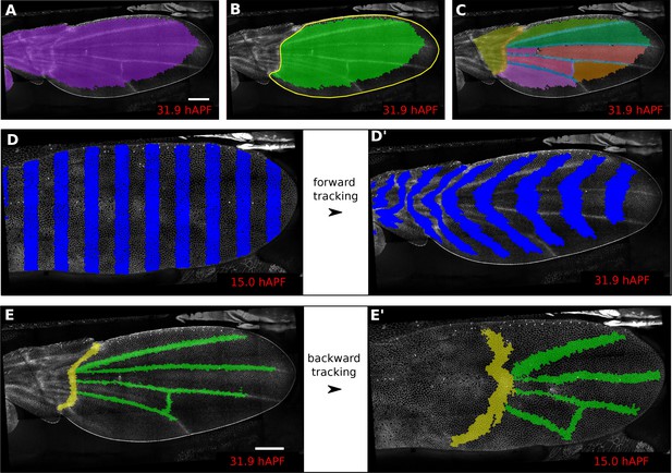
Regions of interest are followed in time by browsing the cell lineages.
(A) Largest population of cells (purple) that remains visible throughout the entire time-lapse. Two cell rows in contact to margin cells were discarded as margin cells are usually not well segmented. (B) Largest blade cell population (green) that remains visible throughout the entire time-lapse. The blade region of interest (yellow line) was defined on the last frame of the time-lapse using a custom Fiji macro (https://github.com/mpicbg-scicomp/tissue_miner/blob/master/fiji_macros/). The underlying cell population was then subset using our lineage browser algorithm. (C) One can define veins and inter-vein regions of interest and apply the same algorithm as in (B). (D–D') Regularly spaced regions of interest automatically selected and followed over time to visualize tissue deformation. (E–E') Here, we make use of the lineage browser routine to trace back the vein positions at 15 hAPF, as they aren't visible yet at 15 hAPF. Scale bar 50 microns.
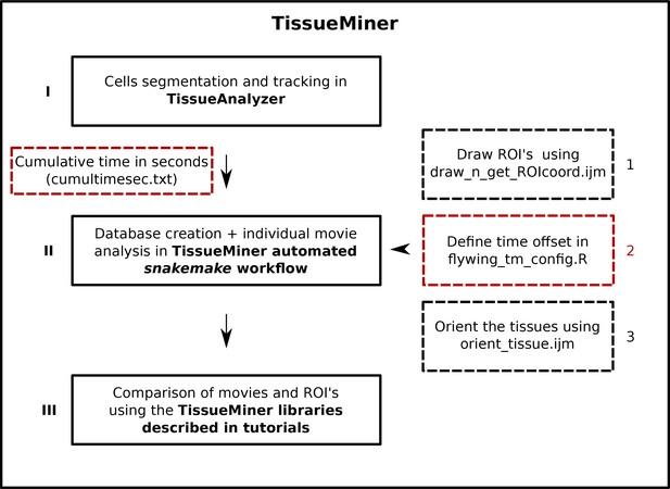
Flow chart of TissueMiner.
Solid lines depict the three main steps to analyze epithelial morphogenesis within TissueMiner. Dashed lines indicate additional inputs to the automated workflow: red boxes represent required inputs and black boxes indicate optional inputs. Arabic numbers indicate the order in which the tools are described in the main text. Cumulative time of the movie must be listed in a text file called cumultimesec.txt and located along with the movie images. The snakemake automated workflow is described in Figure 7.
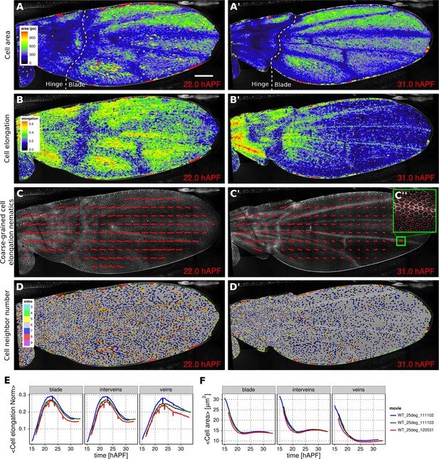
Patterned cell state properties in the developing pupal wing of Drosophila.
(A–D') Cell state patterns at 22 hr and 31 hr after puparium formation (hAPF). (A–A') Color-coded cell area. (B–B') Color-coded cell elongation. The magnitude of cell elongation corresponds to the norm of the cell elongation nematic tensor. (C–C'') Coarse-grained pattern of cell elongation nematics and (C'') cell elongation nematics represented as bars on each individual cell. The wing was divided into adjacent square-grid elements of 33x33 microns in which cell elongation nematics were averaged. (D–D') Color-coded representation of the cell neighbor number. (E) Time evolution of the average cell area in different regions of interest: wing blade (Figure 1B), veins (Figure 1E), and inter-vein regions. (F) Time evolution of the average cell elongation magnitude in the blade, veins and inter-vein regions. Scale bar: 50 microns.
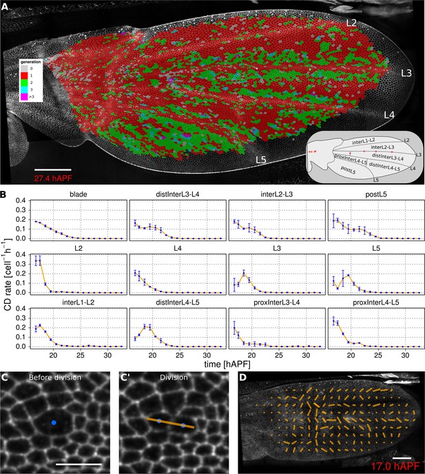
Visualization of cell generations and cell divisions.
(A) Color-coded pattern of cell generations. The wing cartoon on the bottom right shows the names of subregions that we analyze in panel B. Scale bar 50 microns. (B) Cell division rate in different regions of interest. To smooth fluctuations, these rates were averaged in discrete time intervals of one hour (TM R-User Manual, section 3.7). We further averaged these rates amongst the three wild-type wings. Error bars depict the standard deviation between wings. Cells divide earlier in veins L2 and L4 than in L3 and L5. Two maxima corresponding to two rounds of divisions are visible in inter-vein regions: interL2-L3, distInterL3-L4 and postL5. (C–C') A dividing cell with its unit nematic depicting the division orientation. Scale bar 10 microns. (D) Coarse-grained pattern of cell division orientation (grid size of 33x33 microns). Scale bar 50 microns.
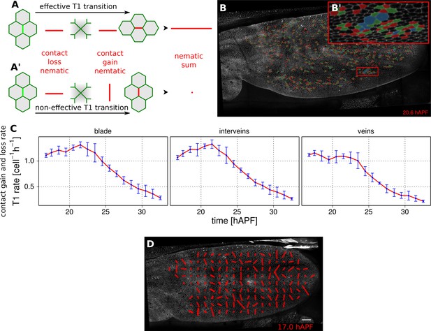
Visualization and quantification of T1 transitions.
(A–A') Cartoon depicting an effective T1 transition (A) that corresponds to cell-contact loss and gain in different directions. Each contact loss or gain is assigned a unit nematic describing its orientation. (B–B') Pattern of cells losing contact (green), gaining contact (red) or both (blue). (C) Rate of neighbor change per cell and per hour in the blade, veins and inter-vein regions of interests. Rates were averaged within discrete time intervals of one hour and further averaged among the 3 WT wings (TM R-User Manual, section 3.8). Error bars depict the standard deviation amongst wings. (D) Coarse-grained pattern of neighbor exchange orientation at 17 hAPF. Cell neighbor change nematics were obtained by summing up unit nematics in each grid elements of 33x33 microns and further averaged in time using a 50 min time window. Scale bar 50 microns.
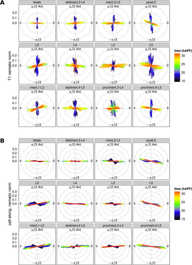
T1 and cell elongation nematic orientation.
(A) Cell neighbor change nematics were averaged at each frame within each region of interest and are represented as bars in a circular diagram. The bar angle indicate the average T1 orientation, and its length (nematic norm) reflects how ordered cell neighbor change nematics are in a given region of interest. Their color depicts the developmental time in hours after puparium formation. (B) Cell elongtation nematics were also averaged at each frame within each region of interest. The average T1 nematic orientation starts to match the average cell elongation nematic orientation from about 22 hAPF (peak of cell stretch) on, when stress-induced PD-oriented T1 dominate over autonomous AP-oriented T1.
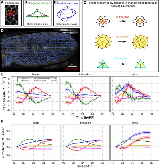
Visualization and quantification of anisotropic cell and tissue deformation.
(A) Triangulation of the cell network: each triangle vertex corresponds to a cell center. (B–B') Cartons depicting triangle pure shear and total tissue shear along the x axis. (C) Cartons depicting shear due to T1 transition, cell division and extrusion. (D) Pattern of local tissue shear rate obtained from the triangulation method. Scale bar 50 microns. (E) shows the average rate of tissue shear (blue) in the blade, interveins and veins, and the corresponding cellular shear contributions (other colors). Shaded regions indicate the standard deviation amongst wings. (F) shows the accumulated tissue shear over time and the accumulated contributions of each type of cellular event. The tissue shear (blue) in veins is orientated along the PD axis and it is higher than in inter-vein regions during most of pupal morphogenesis. It leads to an extension along the PD axis and to a narrowing along the anterior-posterior (AP) direction. By the end of the movie, accumulated tissue shear (blue) is almost twice as high in veins as in inter-vein regions. Shaded regions represent the standard deviation amongst wings.
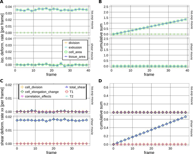
Measurements of cell and tissue deformation from two computer-generated sheets of hexagonal cells.
(A–D) One dataset corresponds to hexagonal cells undergoing a constant isotropic expansion rate of 3.50 10–2 per frame, and the other corresponds to hexagonal cells undergoing constant pure shear rate of 1.75 10–2 per frame. These datasets are termed iso.exp movie and shear movie respectively in graphs. There isn't any topological change. To keep consistent sets of cells in time, we filtered out cells that become in contact to the image border. We then performed our measurement on these tracked regions of about 50 cells in the shear movie and about 100 cells in the iso.exp movie. (A) Relative tissue area changes (blue) and its decomposition into cell area changes (green), cell number increase by divisions (orange) and cell number descrease by extrusions (cyan). Their corresponding cumulative sums are shown in (B). (C) shows the average tissue shear (blue) and its decomposition into cellular shear contributions (other colors). Their corresponding cumulative sums are shown in (D).
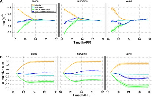
Tissue isotropic deformation and cellular contributions in different regions.
(A) Relative rates of tissue area changes (blue) averaged over 3 WT wings for the blade, veins and interveins, and its decomposition into cell area changes (green), cell number increase by divisions (orange) and cell number descrease by extrusions (cyan). Their corresponding cumulative sums are shown in (B). (B) Cumulative tissue area changes and its cellular contributions. Shaded regions represent the standard deviation amongst wings.
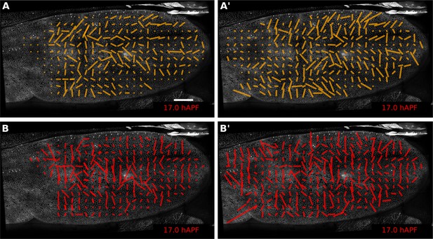
Comparison of patterns of cell event orientation with their correponding quantitative patterns of shear.
(A–A') Coarse-grained patterns of cell division orientation (A) and of shear contributed by cell division (A'). The pattern shown in (A) was obtained by summing up cell division nematics in each grid element and by further averaging in time. The pattern shown in (A') was obtained by averaging the shear nematics in each grid element and by further averaging in time. (B–B') Coarse-grained patterns of neighbor-change orientation (B) and of shear contributed by neighbor changes (B'). These patterns were obtained similarly as for cell divisions. Only the shear patterns (A' and B') obtained with the triangulation method provide a quantitative measurement of the local deformation induced by each type of cellular event. Square-grid size of 26x26 microns. Time averaging covering about 55 min (11 frames) in each grid element. Scale bar 50 microns.
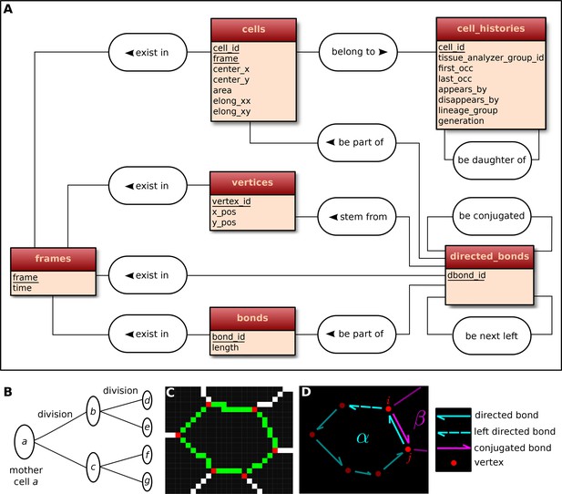
Construction of the relational database of TissueMiner.
(A) Conceptual scheme of the database. Entities (square boxes) are related to other entities by associations (rounded boxes). Each entity contains an identifier (underlined) that uniquely defines each record. The database can be implemented by converting entities into tables (see appendix 1 and Figure 6—figure supplement 2). (B) Cell lineage trees are stored in the database: upon division a mother cell identifier a gives rise to two new daughter cell identifiers b and c. {a,b,c,d,e,f,g} defines one lineage group. (C) A pixelated cell contour in the 2D cell network: green=bond pixels, red=vertex pixels, white=other cell network pixels. (D) Vectorized representation of the cell shown in (C). To preserve the topology of the cell network, directed bonds (cyan) are defined from within a given cell alpha and ordered anticlockwisely along the cell contour. Each directed bond is complemented by a conjugated bond (magenta) and is linked to it next counter-clockwise follower (dashed).

Tracked cells identified by unique colors in TissueAnalyzer.
(A) shows two consecutive frames depicting colored-tracked cells from a time-lapse movie processed with TissueAnalyzer. Each cell is assigned a color identifier that uniquely defines it in the course of the time-lapse. One pixel wide cell-cell interfaces are visible in white on the raster image.
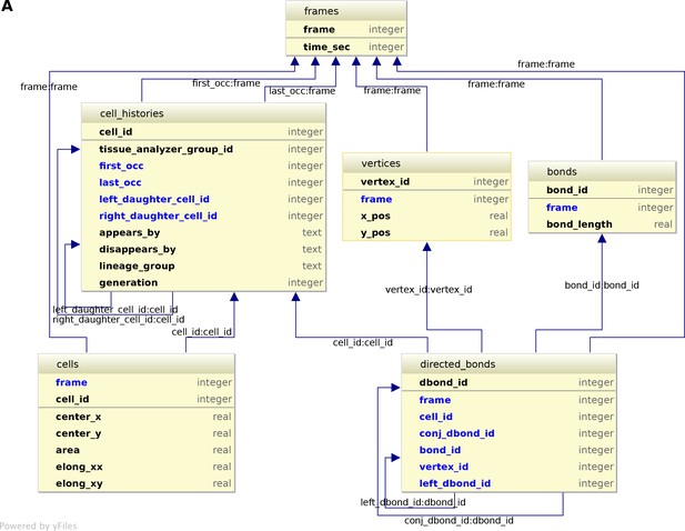
Logical scheme of the relational database.
(A) The conceptual scheme shown in Figure 6A can be automatically converted to a logical scheme shown here by using softwares such as IntelliJDEA or MySQL workbench. The rules of conversion are briefly evoked in appendix 1. The entities defined in the conceptual scheme are converted into tables containing one primary key (upper part of the table) that uniquely defines each record in the table, the properties of each record, and the foreign keys (arrows). Foreign keys are properties of one table pointing to the primary key of a related table (ex: conj_dbond_id:dbond_id means that the conj_dbond_id column is a foreign key whose values must be defined in the dbond_id column of the dbonds table). As a consequence of logical contraints by foreign keys, tables harbor more columns that one expected from looking at Figure 6A. This logical scheme now shows all tables and columns of the database. This scheme is implemented in physical SQLite tables can are indexed for the sake of performance (see CreateDbFromParser.R on https://github.com/mpicbg-scicomp/tissue_miner).
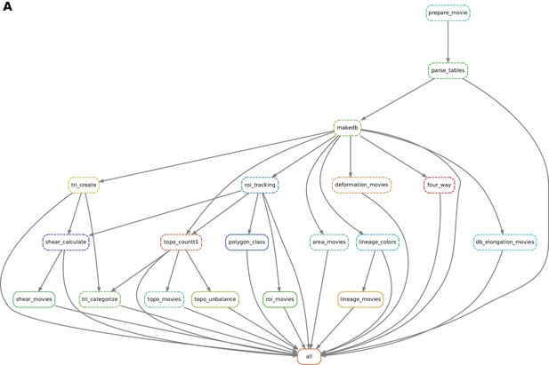
Automated workflow using snakemake.
(A) The snakemake engine can generate a directed acyclic graph (DAG) where we show an example here. This graph represents both the execution dependency (grey arrows) and the execution state of the workflow (solid or dashed line). Each box corresponds to an execution rule, namely a program to be run along with required input(s) and expected output(s). This DAG can be generated at any time when running the workflow (see documentation). Solid lines indicate the rules that have not been executed yet, whereas dashed lines depict completed jobs. The first rule to be executed is called 'prepare_movie': it prepares the tracked images from TissueAnalyzer to be converted by the parser into tables of values containing all necessary entities along with their properties ('parse_tables' rule). Then the 'make_db' rule is executed for building the database. Following the grey arrows can one navigate into the next steps of the workflow. The 'roi_tracking' rule filters out cells in contact to margin cells including user-defined regions of interest, and the 'roi_movie' rule allows us to visualize regions of interest over time. The 'deformation_movies' and 'db_elongation_movies' rules generate annotated movies to visualize the deformation of the tissue and the cell state properties (area, elongation). The 'four_way' rule detects four-way vertices and performs basic statistics on vertices. The 'tri_create' rule performs the triangulation of the network for further shear calculation and visualization ('shear_calculate' and 'shear_movies'). It also enables triangle tracking and mapping to each type of cell event ('tri_categorize'). The 'topo_countT1' rule detects neighbor changes that are not due to division or extrusion, and categorizes them into gained or lost neighbors. The 'topo_movies' rule allows one to visualize the coarse-grained rates of division and neighbor changes on the tissue. The 'topo_unbalance' rule is a quality check to verify that the number of gained neighbors is similar to the number of lost neighbors. The 'polygon_class' rule performs the cell-neighbor number count. The 'lineage_colors' rule allows us to optimize the color of each lineage group such that adjacent lineage groups always have different colors. Finally, the 'lineage_movies' rule allows one to visualize lineage groups and cell generations on the tissue. The rule 'all' checks that all upstream jobs have been completed.
Videos
HOWTO: drawing ROI’s.
https://doi.org/10.7554/eLife.14334.006Visualizing tissue deformation by using vertical stripes.
https://doi.org/10.7554/eLife.14334.007HOWTO: Orienting a tissue.
https://doi.org/10.7554/eLife.14334.008Color-coded cell area pattern.
https://doi.org/10.7554/eLife.14334.010Color-coded cell elongation norm pattern.
https://doi.org/10.7554/eLife.14334.011Coarse-grained cell elongation pattern.
https://doi.org/10.7554/eLife.14334.012Color-coded cell packing pattern.
https://doi.org/10.7554/eLife.14334.013Color-coded cell generation pattern.
https://doi.org/10.7554/eLife.14334.014Color-coded cell division pattern in veins and by time intervals.
https://doi.org/10.7554/eLife.14334.016Coarse-grained cell division pattern.
https://doi.org/10.7554/eLife.14334.017Coarse-grained cell rearrangement pattern
https://doi.org/10.7554/eLife.14334.020Computer-generated hexagonal cells with an imposed shear rate.
https://doi.org/10.7554/eLife.14334.025Computer-generated hexagonal cells with an imposed isotropic expansion rate.
https://doi.org/10.7554/eLife.14334.026Tables
Cardinalities per association.
| Entity A | Entity B | Association (A->B) | Cardinality A->B | Cardinality B->A |
|---|---|---|---|---|
| cell_histories | cell_histories | to be daughter of | [0,1] | [0,n] |
| cells | cell_histories | to belong to | [1,1] | [1,n] |
| cells | frames | to exist in | [1,1] | [1,n] |
| directed_bonds | cells | to be part of | [1,1] | [1,n] |
| directed_bonds | directed_bonds | to be conjugated | [1,1] | [1,1] |
| directed_bonds | directed_bonds | to be next left | [1,1] | [1,1] |
| directed_bonds | frames | to exist in | [1,1] | [1,n] |
| directed_bonds | bonds | to be part of | [1,1] | [1,n] |
| directed_bonds | vertices | to stem from | [1,1] | [1,n] |
| vertices | frames | to exist in | [1,1] | [1,n] |
| bonds | frames | to exist in | [1,1] | [1,n] |


