Tracking transcription factor mobility and interaction in Arabidopsis roots with fluorescence correlation spectroscopy
- North Carolina State University, United States
- University of California, Irvine, United States
- Howard Hughes Medical Institute, Duke University, United States
- Wageningen University, Netherlands
Figures
Figure 1 with 1 supplement

Diffusion coefficients obtained by performing RICS on SHR:SHR-GFP in shr2.
(a) Schematic showing image acquisition and RICS analysis. (Left) A time series of 100 frames (time points) acquired using predetermined imaging parameters (Table 1). (Middle) Autocorrelation function (ACF) calculated from the time series. Red represents a high ACF value, blue represents a low ACF value. (Right) Fit of the ACF to a Gaussian diffusion model to calculate the diffusion coefficient. (b–d) Representative images of SHR:SHR-GFP in shr2 taken in regions containing the vasculature and endodermis (b), endodermis only (c), vasculature and QC (d). Cell walls are marked in red using propidium iodide (PI). Below each image is its ACF fit using the Gaussian model and the calculated diffusion coefficient for that representative image. (d) 128x128 pixel region of interest (ROI) used for RICS (white frame). (e) Bar graph showing average diffusion coefficients of 35S:GFP (n = 34), SHR:SHR-GFP in shr2 (n = 40) for vasculature and endodermis, n = 19 for endodermis, n = 20 for vasculature and QC) and SHR:SHR-GFP in SCRi (vasculature and endodermis, n = 14). Groups that have different symbols are significantly different from each other and from the 35S:GFP line (Wilcoxon with Steel-Dwass, p<0.05). Error bars are s.e.m. Source data is provided in Figure 1—source data 1–4 .
-
Figure 1—source data 1
Diffusion coefficient of 35S:GFP line obtained using RICS with the Zeiss 780 and Zeiss 710 instruments.
- https://doi.org/10.7554/eLife.14770.004
-
Figure 1—source data 2
Diffusion coefficient of SHR:SHR--GFP in shr2 line obtained using RICS with the Zeiss 780 and Zeiss 710 instruments.
- https://doi.org/10.7554/eLife.14770.005
-
Figure 1—source data 3
Diffusion coefficient of SHR:SHR--GFP in SCRi line obtained using RICS with the Zeiss 780 instrument.
- https://doi.org/10.7554/eLife.14770.006
-
Figure 1—source data 4
Statistical analysis of diffusion coefficients obtained by RICS.
- https://doi.org/10.7554/eLife.14770.007
Figure 1—figure supplement 1
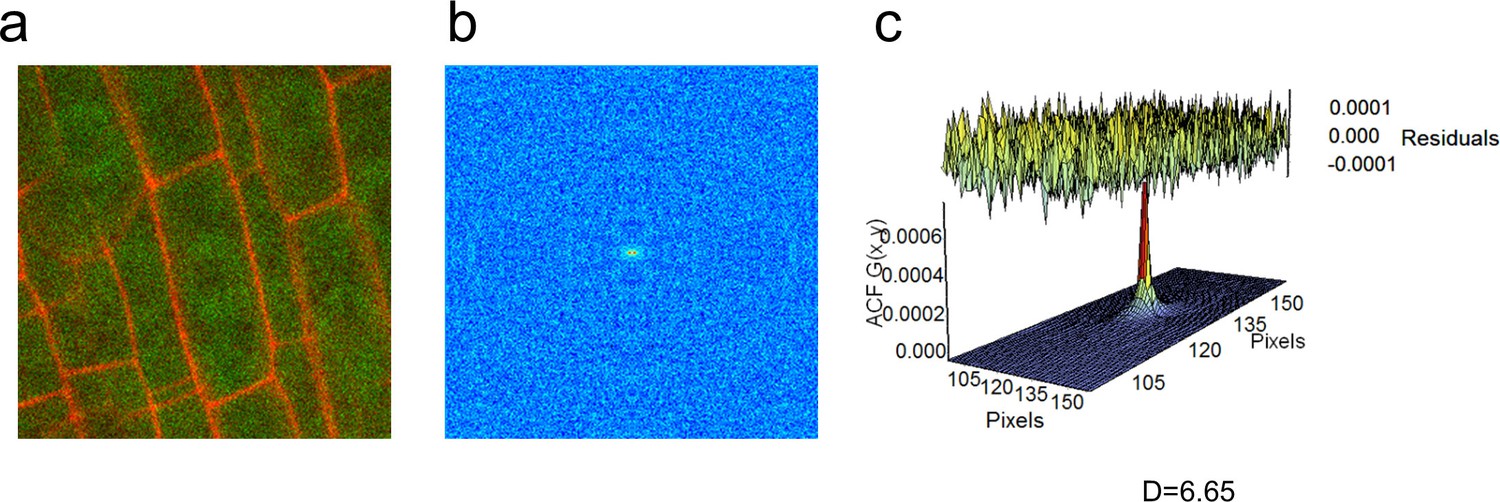
RICS analysis on the 35S:GFP line.
(a) Region of interest of 35S:GFP in vasculature cells. (b) Autocorrelation function (ACF) calculated using RICS. Red represents a high ACF value, blue represents a low ACF value. (c) Fit of diffusion model and calculation of diffusion coefficient from the ACF. Residuals of fit are shown at top of graph.
Figure 2 with 1 supplement
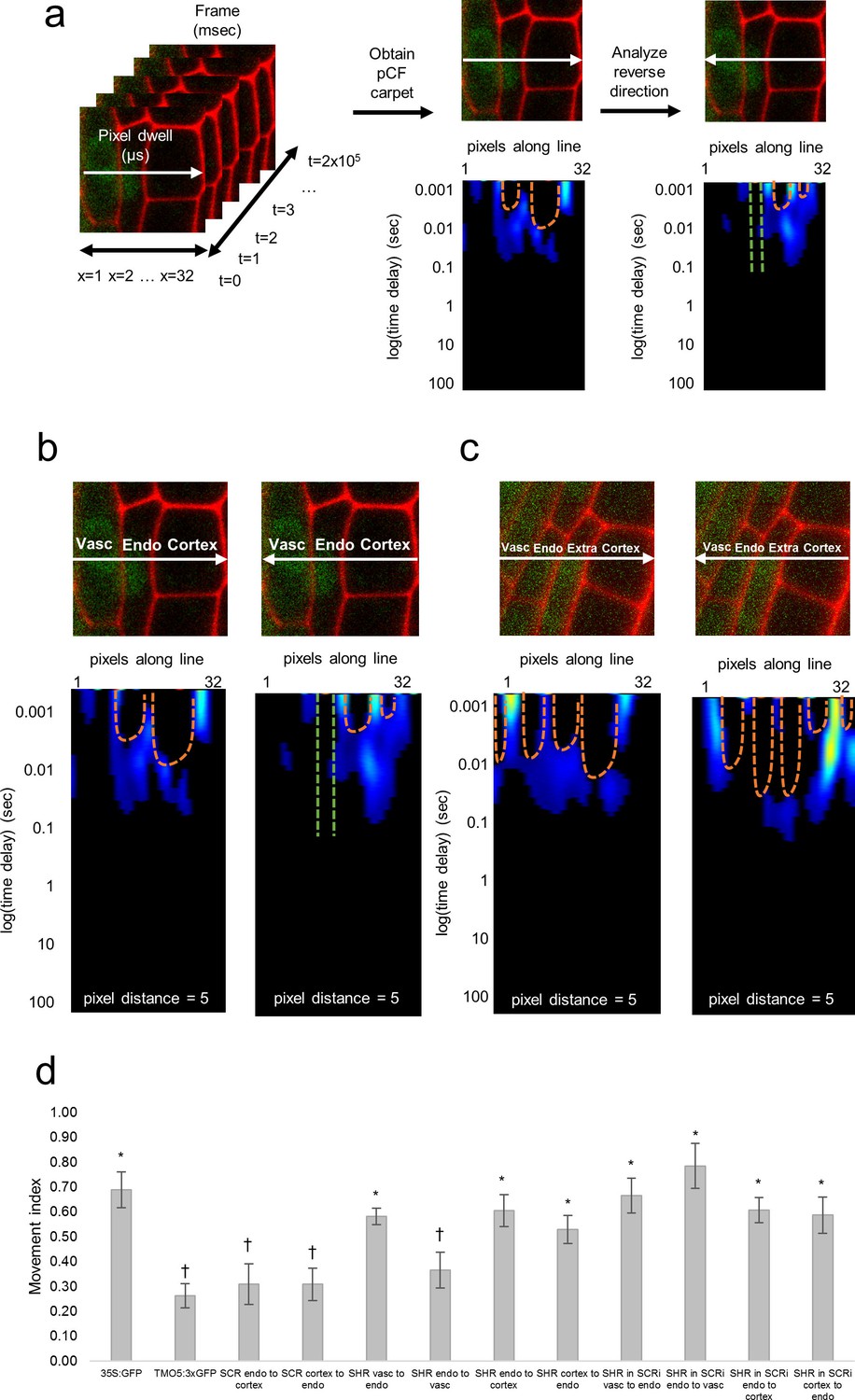
Pair correlation function (pCF) analysis showing direction of SHR movement.
(a) Schematic of image acquisition and pCF analysis. (Left) Line scans acquired using predetermined imaging conditions (Table 1). Carpets of the forward (middle) and reverse (right) pCF analysis. The orange arch indicates delayed movement, while the absence of an arch (green lines) indicates no movement. (b) pCF analysis of SHR:SHR-GFP in shr2. Cell walls are marked with PI. Lines indicate the laser path going across the vasculature, endodermis, and cortex. pCF carpets for each direction are shown. Orange arches indicate movement. (c) pCF analysis of SHR:SHR-GFP in SCRi. Cell walls are marked with PI. Lines indicate the laser path across the vasculature, endodermis, the extra layer, and the cortex. pCF carpets for each direction are shown. Orange arches indicate movement. (d) Bar graph showing average movement index of 35S:GFP (n = 15), TMO5:3xGFP (n = 19), SCR:SCR-GFP (n = 14), SHR:SHR-GFP in shr2 (n = 20) between vasculature and endodermis, n = 22 between endodermis and cortex), and SHR:SHR-GFP in SCRi (n = 14 between vasculature and endodermis, n = 17 between endodermis and cortex). Stars denote groups that are different from TMO5:3xGFP, crosses indicate groups that are different from 35S:GFP (Wilcoxon with Steel-Dwass, p<0.05). Error bars are s.e.m. Source data is provided in Figure 2—source data 1 and 2.
-
Figure 2—source data 1
pCF of 35S:GFP, TMO5:3xGFP, SCR:SCR-GFP, SHR:SHR-GFP in shr2, and SHR:SHR-GFP in SCRi lines.
- https://doi.org/10.7554/eLife.14770.011
-
Figure 2—source data 2
Statistical analysis of movement index obtained by pCF.
- https://doi.org/10.7554/eLife.14770.012
Figure 2—figure supplement 1
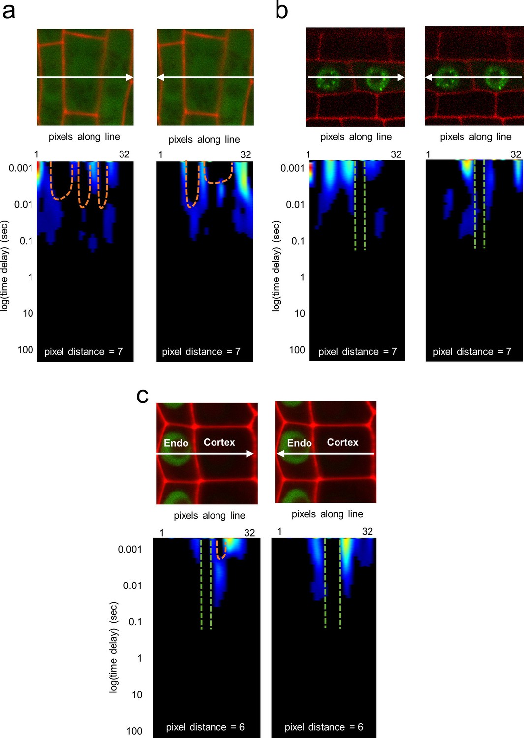
Pair correlation function analysis of 35S:GFP, SCR:SCR-GFP, and TMO5:3xGFP.
(a) pCF analysis of 35S:GFP in vasculature cells. Cell walls are marked with PI. Orange arches indicate movement. (b) pCF analysis of TMO5:3xGFP in vasculature cells. Cell walls are marked with PI. Green lines indicate no movement. (c) pCF analysis of SCR:SCR-GFP in endodermal and cortical cells. Cell walls are marked with PI. Orange arches indicate movement. Green lines indicate no movement.
Figure 3

N&B analysis of the SHR oligomeric state.
(a) Schematic of image acquisition and N&B analysis. (Left) Image acquisition for N&B is the same as for RICS analysis. (Middle) The mean and variance of intensity used to calculate the brightness and number of particles. (Right) The background brightness (red) set to 1 by adjusting the S-factor (Table 2). The monomer (blue) positioned at the predetermined brightness of monomeric GFP (Table 2). Homodimer (green) particles shown to be twice as bright as the monomer. (b, c, d) 35S:GFP used to determine the molecular brightness of monomeric GFP (b, e, h) Region of interest selected for N&B analysis of 35S:GFP, SHR:SHR-GFP in shr2, and SHR:SHR-GFP in SCRi. Cell walls are marked with PI. Note that the extra layer in (h) is a result of the SCRi background. (c, f, i) Brightness vs intensity for 35S:GFP, SHR:SHR-GFP in shr2, and SHR:SHR-GFP in SCRi. The red, blue, green boxes indicate the autofluorescence (B = 1), monomer (B = ε = 0.28 ± 0.01) and homodimer (B = 2*ε), respectively. (d, g, j) Color-coding of the brightness for 35S:GFP, SHR:SHR-GFP in shr2, and SHR:SHR-GFP in SCRi. Red, blue, and green represent background (autofluorescence), monomer, and homodimer, respectively. (k) Bar graph showing average percent of SHR homodimer for SHR:SHR-GFP in vascular cells (n = 40), SHR:SHR-GFP in endodermal cells (n = 19), and SHR:SHR-GFP in SCRi (n = 14). Error bars are s.e.m. Star denotes sample that is significantly different from the other two (Wilcoxon with Steel-Dwass, p<0.05). Source data is provided in Figure 3—source data 1–3.
-
Figure 3—source data 1
Oligomeric state of SHR:SHR--GFP in shr2 line obtained using N&B with the Zeiss 780 and Zeiss 710 instruments.
- https://doi.org/10.7554/eLife.14770.015
-
Figure 3—source data 2
Oligomeric state of SHR:SHR--GFP in SCRi line obtained using N&B with the Zeiss 780 instrument.
- https://doi.org/10.7554/eLife.14770.016
-
Figure 3—source data 3
Statistical analysis of the oligomeric state of SHR collected using N&B.
- https://doi.org/10.7554/eLife.14770.017
Figure 4 with 2 supplements
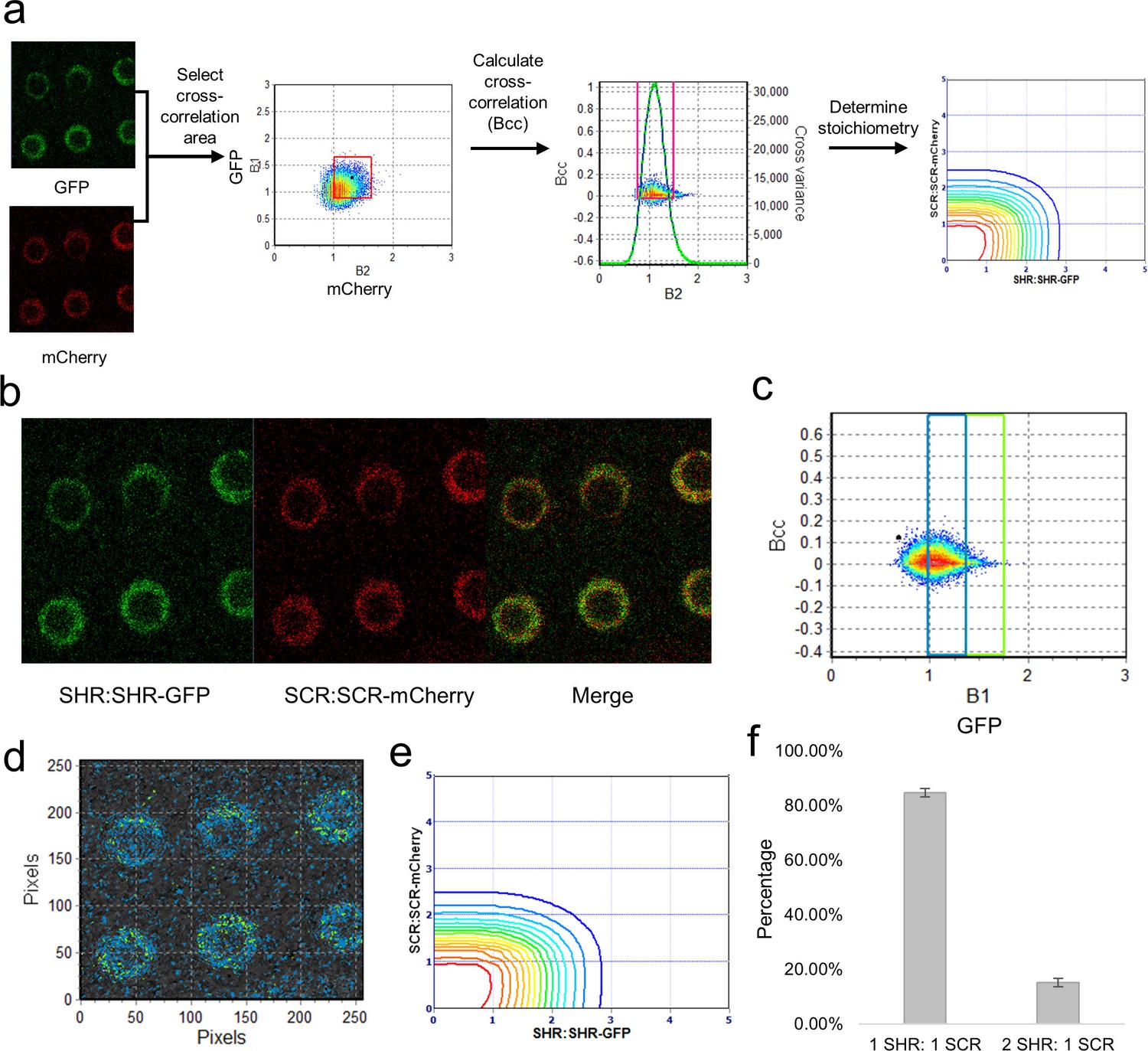
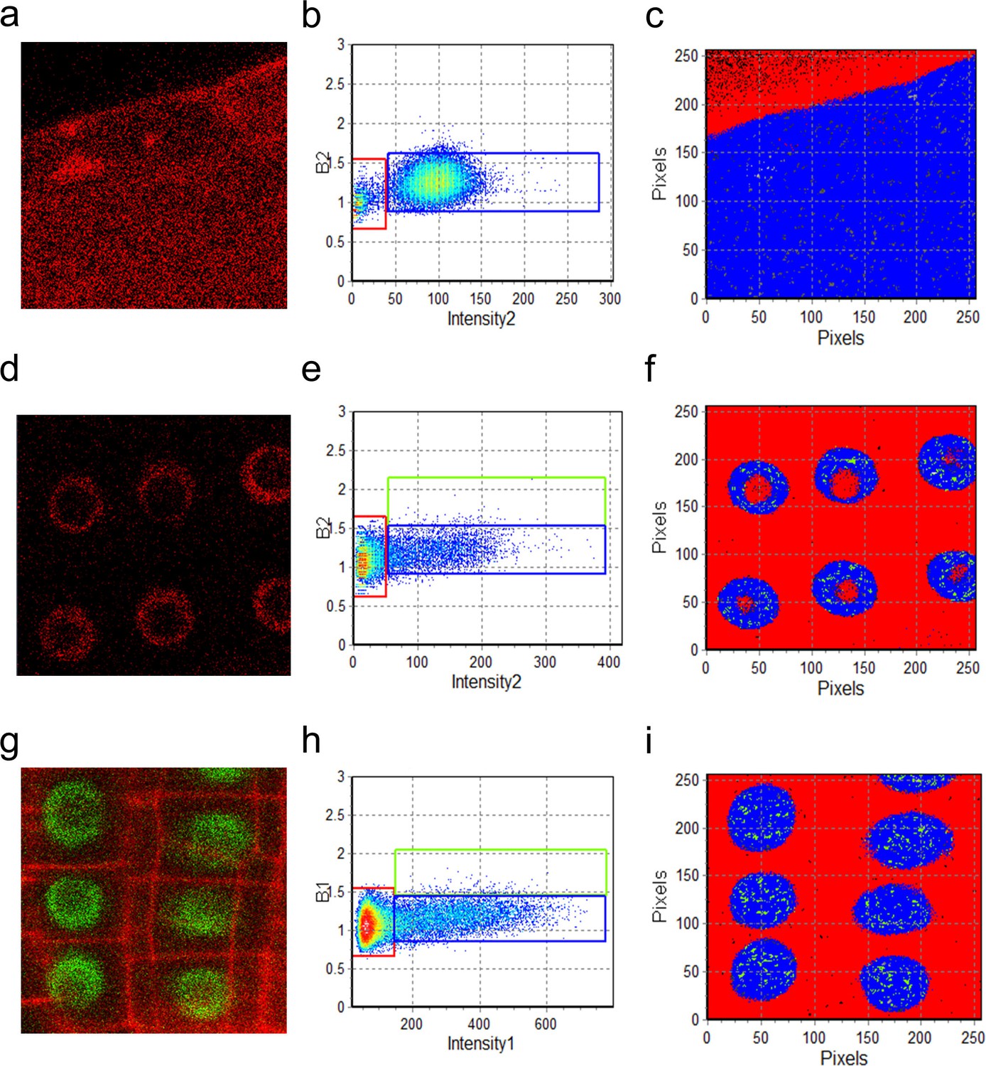
Cross-N&B analysis of a SHR/SCR double-tagged line.
(a) Schematic of cross N&B analysis. (Left) A double-tagged line used for imaging. The B1 (GFP brightness) vs B2 (mCherry brightness) graph is used to select the region for cross-correlation. (Middle) The brightness cross-correlation (Bcc) used to determine GFP pixels that cross-correlate with mCherry pixels. (Right) Stoichiometry plot that displays the protein complexes detected in the image. (b) Expression of SHR:SHR-GFP/SCR:SCR-mCherry marker line in root endodermis. (c) Bcc vs B1 graph for SHR. The blue and green boxes represent the SHR monomer and homodimer, respectively, that form a complex with SCR. (d) Color-coding of the cross brightness of the SHR:SHR-GFP/SCR:SCR-mCherry line. Blue represents SHR monomer binding SCR monomer, while green represents SHR homodimer binding SCR monomer. (e) Stoichiometry histogram from cross N&B analysis. The orange line at (1,1) represents a high proportion of monomeric SHR bound to monomeric SCR (84.77% ± 1.58%), while the green line at (2,1) represents a lower proportion of homodimeric SHR bound to monomeric SCR (15.23% ± 1.58%). (f) Bar graph showing average percentages of the 1:1 and 2:1 SHR-SCR complex (n = 17). Error bars are s.e.m. Source data is provided in Figure 4—source data 1 and 2.
-
Figure 4—source data 1
Oligomeric state of SCR:SCR-GFP and SCR:SCR-mCherry lines obtained using N&B with the Zeiss 780 instrument.
- https://doi.org/10.7554/eLife.14770.023
-
Figure 4—source data 2
Stoichiometry of the SHR:SHR-GFP/SCR:SCR-mCherry complex obtained using cross N&B with the Zeiss 780 instrument.
- https://doi.org/10.7554/eLife.14770.024
Figure 4—figure supplement 1
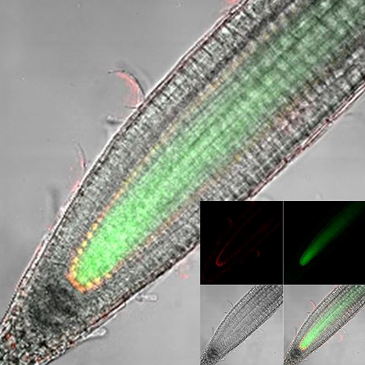
Longitudinal confocal root sections of SHR:SHR-GFP/SCR:SCR-mCherry line.
Inset: Red (SCR:SCR-mCherry), green (SHR:SHR-GFP), BF, and merged channels.
Figure 4—figure supplement 2
N&B analysis of UBQ10 and SCR oligomeric state.
(a, d, g) Region of interest of UBQ10:mCherry, SCR:SCR-mCherry, and SCR:SCR-GFP in the root. Both SCR:SCR-mCherry (d) and SCR:SCR-GFP (g) are shown in the endodermis. (b, e, h) (b, e, h) Brightness (B) vs intensity graphs for UBQ10:mCherry, SCR:SCR-mCherry, and SCR:SCR-GFP. The red, blue, and green boxes indicate the autofluorescence (B=1), monomer (B1 = = 0.28 ± 0.01 for GFP; B2 = = 0.34 ± 0.02 for mCherry) and homodimer (B1 = 2*monomeric B1 for GFP; B2 = 2*monomeric B2 for mCherry) (Table 2). (c, f, i) Color-coding of the distribution of the brightness of UBQ10:mCherry, SCR:SCR-mCherry, and SCR:SCR-GFP. Red, blue, and green represent autofluorescence, monomer, and homodimer respectively.
Figure 5 with 2 supplements
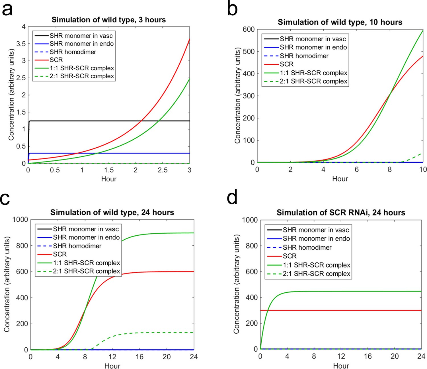
Mathematical model simulations of SHR and SCR illustrate how reduction of SCR affects the formation of SHR homodimer and SHR-SCR complex.
(a, b, c) Model simulations of wild type showing how (a) SCR and the 1:1 SHR-SCR complex greatly increase in the first 3 hr, (b) SHR homodimer and the 2:1 SHR-SCR complex do not form until around 9 hr, (c) the entire system reaches a steady state between 18–24 hr. (d) Model simulations of SCR RNAi showing a reduction in SHR homodimer, SCR, 1:1 SHR-SCR complex, and 2:1 SHR-SCR complex levels after 24 hr. The model outcomes show SHR in the vasculature (black), SHR monomer in the endodermis (solid blue), SHR homodimer (dashed blue), SCR (red), 1:1 SHR-SCR complex (solid green), and 2:1 SHR-SCR complex (dashed green). Parameter values and initial conditions are given in Supplementary file 3. Source data is provided in Figure 5—source data 1 and 2.
-
Figure 5—source data 1
Sobol total effects indices computed for SHR-SCR mathematical model.
- https://doi.org/10.7554/eLife.14770.028
-
Figure 5—source data 2
Area measurements of vascular and endodermal cells.
- https://doi.org/10.7554/eLife.14770.029
Figure 5—figure supplement 1
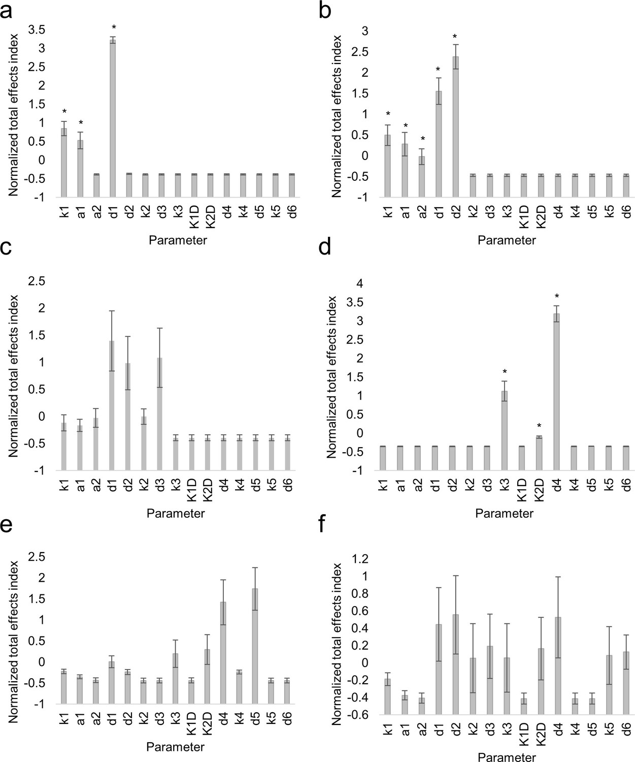
Sensitivity analysis of mathematical model of SHR and SCR.
Bar graphs showing average Sobol total indices (n = 10) for SHR in vasculature (a), SHR monomer in endodermis (b), SHR homodimer (c), SCR (d), 1:1 SHR-SCR complex (e), and 2:1 SHR-SCR complex (f). Indices were normalized to mean 0, variance 1 before averaging. Bars represent s.e.m. Stars denote parameters that have significantly higher total effects indices (Wilcoxon with Steel-Dwass, p<0.10). Source data is provided in Figure 5—source data 1.
Figure 5—figure supplement 2
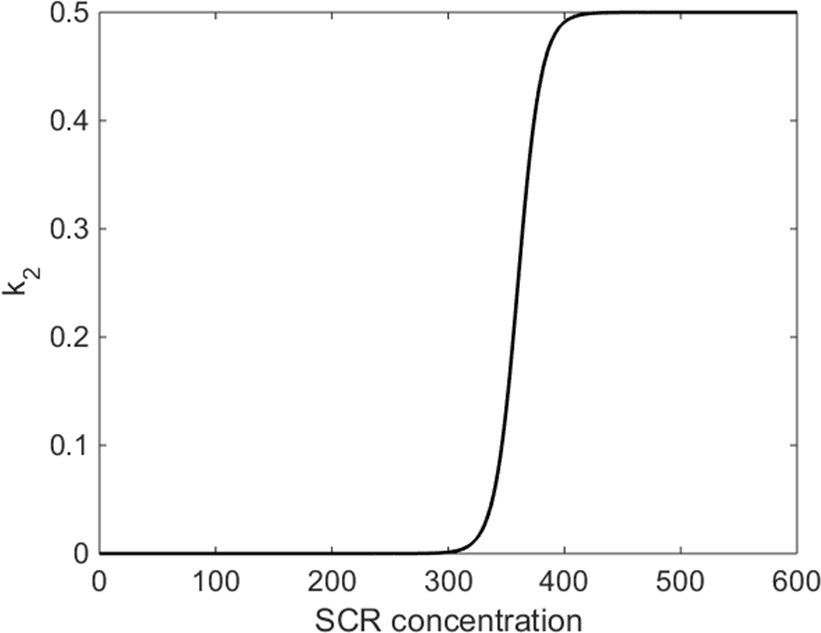
Functional form of k2 parameter in mathematical model.
k2 is the rate of SHR homodimer formation and depends on the concentration of SCR. Once SCR passes a critical value (C0 = 360), SHR homodimer formation switches on. The homodimer formation rate has a maximum value of L = 0.5.
Tables
Table 1
Recommended imaging conditions for RICS and N&B.
| Method | Pixel size (μm) | Pixel dwell time (μs) | Line scan time (ms) | Number of frames | Image size | Laser intensity | Gain | |
|---|---|---|---|---|---|---|---|---|
| RICS | 0.05 to 0.1 | 12.61 or 25.21 | 7.56 or 15.13 | 50 to 100 | 256x256 | 1.0% to 4.0% | 800 to 1000 | |
| N&B | 0.1 | 12.61 or 25.21 | 7.56 or 15.13 | 50 to 100 | 256x256 | 1.0% to 12% | 800 to 1000 | |
Table 2
N and B parameters for SimFCS software analysis. SEM is given.
| Confocal model and objective | S-factor (green channel) | S-factor (red channel) | Monomer brightness (green channel) (counts/pixel dwell/molecule) | Monomer brightness (red channel) (counts/pixel dwell/molecule) | Cursor size |
|---|---|---|---|---|---|
| LSM 780, 40 x 1.2 NA water | 1.34 ± 0.02 (n = 17) | 1.00 ± 0.01 (n = 24) | 0.28 ± 0.01 (n = 13) | 0.34 ± 0.02 (n = 7) | 42 ± 0.69 (n = 13) |
| LSM 710, 40 x 1.2 NA and 63 x 1.2 NA water | 0.92 ± 0.004 (n = 20) | N/A* | 0.24 ± 0.01 (n = 20) | N/A* | 50 (n = 20) |
| Source data is provided in Figure 2—source data 1 (Monomer brightness for green channel and cursor size); Table 2—source data 2 (S-factor, green channel); and Table 2—source data 3 (Monomer brightness and S-factor, red channel) *Red channel data was not collected on the LSM 710 | |||||
-
Table 2—source data 1
Monomeric brightness of 35S:GFP line obtained using N&B with the Zeiss 780 and Zeiss 710 instruments.
- https://doi.org/10.7554/eLife.14770.019
-
Table 2—source data 2
S-factor of the 35S:GFP background line obtained using N&B with the Zeiss 780 and Zeiss 710 instruments.
- https://doi.org/10.7554/eLife.14770.020
-
Table 2—source data 3
S-factor of the UBQ10:mCherry background line and monomeric brightness of UBQ10:mCherry line obtained using N&B with the Zeiss 780 instrument.
- https://doi.org/10.7554/eLife.14770.021
Additional files
-
Supplementary file 1
Results of shapiro-wilk goodness of fit (GoF) test on RICS and N&B data.
- https://doi.org/10.7554/eLife.14770.032
-
Supplementary file 2
PSF beam waist values.
- https://doi.org/10.7554/eLife.14770.033
-
Supplementary file 3
Parameter values used for mathematical modeling.
- https://doi.org/10.7554/eLife.14770.034
-
Supplementary file 4
MATLAB code used to compute the Sobol total effects index.
- https://doi.org/10.7554/eLife.14770.035
Download links
A two-part list of links to download the article, or parts of the article, in various formats.
Downloads (link to download the article as PDF)
Open citations (links to open the citations from this article in various online reference manager services)
Cite this article (links to download the citations from this article in formats compatible with various reference manager tools)
Tracking transcription factor mobility and interaction in Arabidopsis roots with fluorescence correlation spectroscopy
eLife 5:e14770.
https://doi.org/10.7554/eLife.14770


