Global, quantitative and dynamic mapping of protein subcellular localization
- Max Planck Institute of Biochemistry, Germany
Figures
Figure 1 with 1 supplement
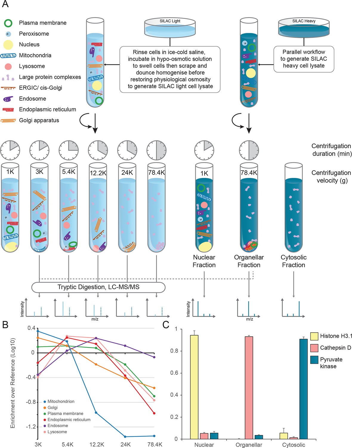
Generation of organellar maps through fractionation profiling.
(A) Metabolically labelled HeLa cells were mechanically lysed to release organelles. Light labelled lysate was then subjected to differential centrifugation at the indicated speeds (RCFMAX) and times (in minutes). Heavy-labelled lysate was centrifuged twice, once at low speed to generate a nuclear-enriched pellet, and again at high speed to generate the organellar pellet; the supernatant was the cytosolic fraction. The heavy organellar ‘reference’ fraction was combined with equal protein amounts of each of the five light membrane sub-fractions and analysed by mass spectrometry, generating SILAC ratios for each protein in all fractions. (B) The SILAC ratios were converted to enrichment over reference. Median values of organellar marker proteins were plotted, showing clearly distinct profiles. (C) In a parallel analysis, the heavy-labelled nuclear, organellar and cytosolic fractions were subjected to label-free mass spectrometric analysis, revealing the global distribution of proteins across these three fractions. Examples of normalized profiles of marker proteins for the nucleus (Histone H3), lysosome (Cathepsin D) and the cytosol (Pyruvate Kinase) are shown. Bars show mean ± SD (n = 6). Please refer to Figure 1—figure supplement 1 for organellar leakage analysis and evaluation of fractionation yield reproducibility.
Figure 1—figure supplement 1

Organellar leakage analysis (A) and fractionation reproducibility (B, C).
(A) Leakage of lumenal contents from endoplasmic reticulum, mitochondria and lysosomes was calculated by quantifying the cytosolic pool of lumenal marker proteins (see Figure 1C, and Materials and methods for further details). For each organelle, a distribution of values was obtained. In all cases there was a large pool of proteins that showed no leakage (<1%). These are probably attached to the organellar membrane, or part of a larger assembly, and thus cannot leak. Conversely, there was a very small number of proteins with very high values (>20%); these are likely to have a genuine cytosolic pool, possibly caused by a cytosolic splice variant not discriminated by the mass spectrometry. In between, there were proteins showing a range of values (1–20%); they are likely to reflect actual organellar leakage. Averages calculated from these middle values are 8.3% for ER, 3.9% for mitochondria, and 2.3% for lysosomes. These very low values suggest that organelles are largely intact. (B) The protein yields of each of the differential centrifugation fractions (see Figure 1A) were calculated using a BCA assay. Yields were converted to % by dividing each fraction by the total yield. This allowed independent experiments to be combined; error bars show the small standard deviations of 6 experiments, highlighting the high reproducibility of the fraction yields. (C) The protein yields of the nuclear, membrane and cytosolic fractions were calculated as in (B), and the small standard deviations of six experiments reveal a similarly high yield reproducibility. In B and C, bars show mean + SD, n=6.
Figure 2 with 2 supplements

Visualization of an organellar map.
Thirty SILAC ratios from six replicate fractionation experiments were combined and subjected to principal component analysis to achieve dimensionality reduction. Projections along the first (x-axis) and third (y-axis) principal components (PCs) provided the optimal separation of clusters. Each scatter point represents a protein. Proximity of proteins indicates similar fractionation behaviour. Marker proteins for organelles are coloured as indicated in the legend, and reveal clustering of proteins belonging to the same organelle. Non-marker proteins are shown as small grey dots. PCs 1–3 account for 64%, 21%, and 12% of the variability in the data, respectively. Please note that the actual resolution of the map is much higher than is apparent in this 2D representation of the full 30-dimensional data set, and most of the seemingly overlapping clusters are in fact separated. Please refer to Figure 2—figure supplement 1 for more detailed cluster annotation, and overlays with external protein sequence feature predictions. Figure 2—figure supplement 2 shows the reproducibility analysis of six replicate organellar maps. The complete organellar assignments, spatial and abundance information can be found in Supplementary file 1 (compact format) and 4 (interactive database).
Figure 2—figure supplement 1
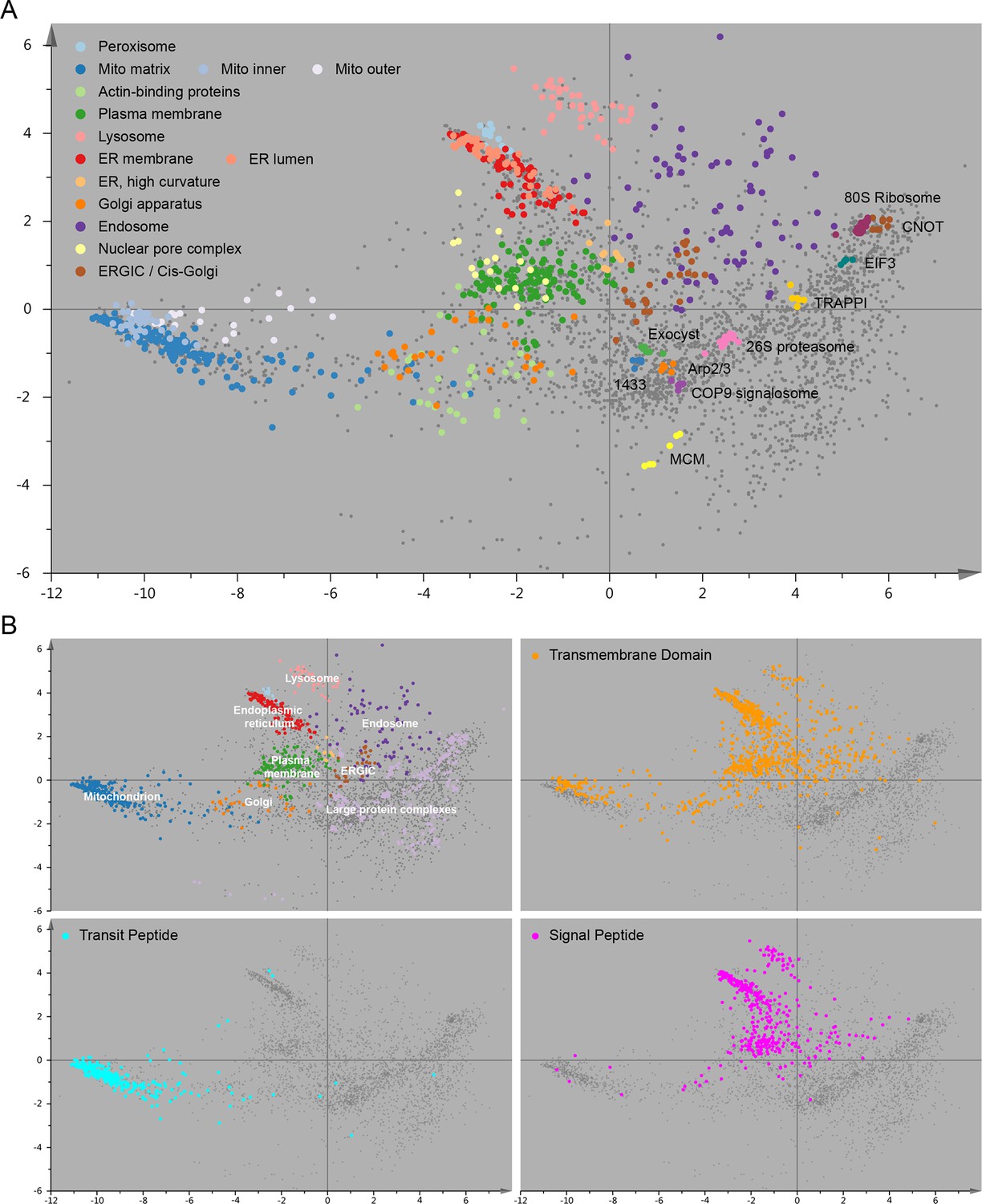
Organellar map with full cluster annotation (A); overlay of an organellar map with external protein sequence feature predictions (B).
(A) Close inspection of the map shown in Figure 2 reveals sub-clustering within the main clusters. The mitochondrial cluster shows separation into outer membrane, inner membrane and matrix proteins; the endoplasmic reticulum is separated into lumenal and membrane proteins. Furthermore, numerous large protein complexes show very tight clustering; a few examples are annotated. In many cases the resolution of this map is sufficiently high to predict constituents of a complex by a ‘neighbourhood analysis’ (Supplementary file 4). Note that the actual resolution of the map (in full dataspace) is much higher than apparent from this 2D principal component analysis. (B) The organellar map shown in Figure 2 was coloured according to UniProt annotations for proteins with transmembrane domains, mitochondrial transit peptide, or signal peptide. The transmembrane domain annotation is almost completely absent from the large protein complex area of the plot, as would be expected. Moreover, the mitochondrial transit peptide annotations cluster, and overlap with our independently derived mitochondrial cluster. Conversely, the signal peptide annotation overlaps with membrane organellar markers, except mitochondria, as would be expected.
Figure 2—figure supplement 2

Reproducibility analysis of organellar maps.
(A) Six individual maps (with five SILAC ratios each) were visualized by PCA as described in Figure 2. Maps were made in pairs (1&2, 3&4, 5&6), on three separate days. Notice the highly reproducible pattern of all maps. (B) Pearson correlation of log2 SILAC ratios in equivalent subcellular fractions from six replicate maps. The average fraction correlation is reported for all 15 pairwise comparisons. The correlation is very high in all cases, and almost identical for intra-day (bold text) and inter-day comparisons. (C) Map concordance, ie the proportion of identical organellar predictions between two replicate maps, shown as a function of prediction confidence. The averages from the three intra-day comparisons (black dots), and 12 inter-day comparisons (red dots) are shown. For example, for two maps made on the same day, 93.7% of all predictions are identical. If a stringency filter is introduced (eg confidence score >8), which retains 77% of the predictions, concordance is increased to 98%. Remarkably, concordance for maps made on different days is almost as high.
Figure 3
Quantitative anatomy of a HeLa cell.
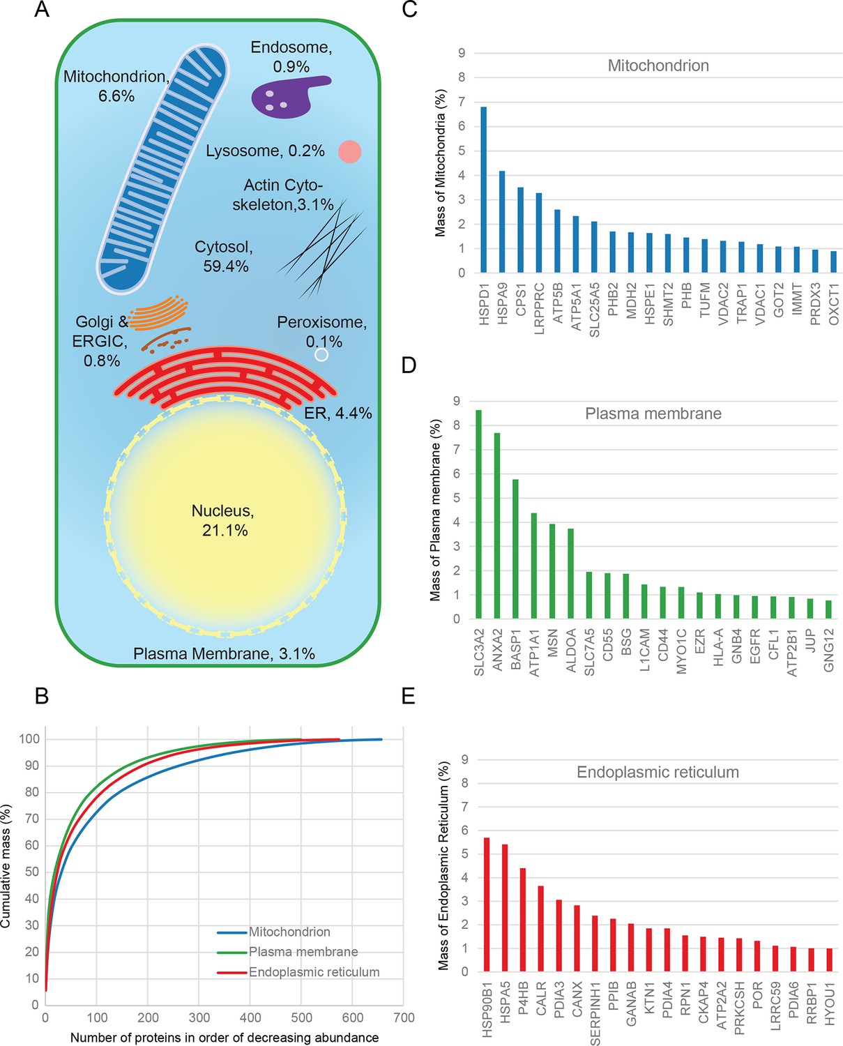
(A) Schematic diagram of a cell where compartments are approximately scaled by their relative contributions to total cell protein mass (not by their volumes). All membranous organelles combined (excluding the nucleus) contribute ca. 16%. For comparison, ribosomes and proteasomes contribute 6% and 1.3%, respectively. The proportion of the ER fraction would increase from 4.4% to ca. 5.4% if attached ribosomes were included. (B) Proteins of major organelles were ranked in order of decreasing abundance, and plotted against their cumulative mass. Very few proteins contribute the majority of organellar protein mass in all three cases. (C–E) Top 20 most abundant proteins in each of the three major organelles, plotted against their contribution to protein organelle mass. The complete quantitative composition of ER, mitochondria, and plasma membrane are shown in Supplementary file 5.
Figure 4 with 3 supplements
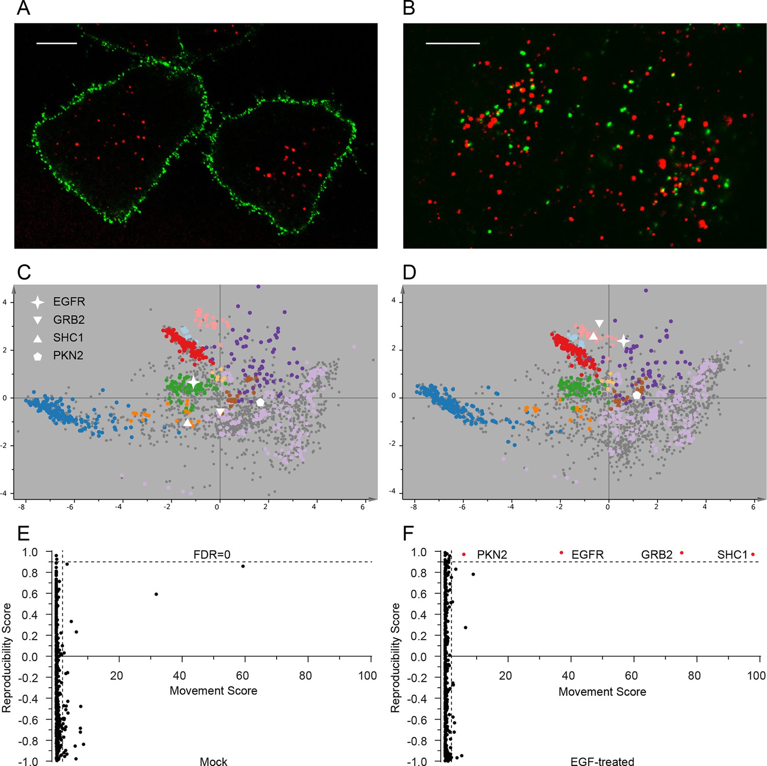
Dynamic organellar maps reveal protein localization changes following EGF stimulation.
(A, B) Fluorescently tagged EGF (green) was pre-bound to HeLa cells on ice, and imaged by confocal microscopy. Lysosomal compartments were visualized with Lysotracker (red). Most of the EGF was at the cell surface (A). Cells were then shifted to 37°C, and incubated for 30 min. EGF had been cleared off the cell surface, and localized predominantly to an endosomal compartment, with little lysosomal co-localization (B). Scale bars = 10 μm. (C) Organellar maps were prepared from untreated HeLa cells, and (D) from cells following 20 min of continuous stimulation with 20 ng/ml EGF. The translocation of the EGFR receptor (star symbol) from plasma membrane to endosomes was captured. Colours indicate organelles as in Figure 2. Maps show the combined data from three replicates each. (E, F) Unbiased identification of significant translocation events triggered by EGF stimulation. Each protein is scored for magnitude of translocation (M score, x-axis) and reproducibility of translocation direction (R score, y-axis) across the three replicates. A MR plot reveals significant translocations in the top right quadrant. Score cut-offs for FDR-control were determined by analysis of a triplicate mock experiment where no genuine translocations are expected (E). Ultra-stringent cut-offs (corresponding to an FDR of 0) were then applied to the EGF treatment experiment (F). Four significant translocations were detected, including EGFR and two known binding partners, GRB2 and SHC1. As the maps in C, D reveal, all move to the endolysosomal cluster. Figure 4—figure supplement 1 provides a schematic of the experimental design. Please refer to Figure 4—figure supplements 2 and 3 for further in-depth analysis of protein localization changes following EGF stimulation.
Figure 4—figure supplement 1
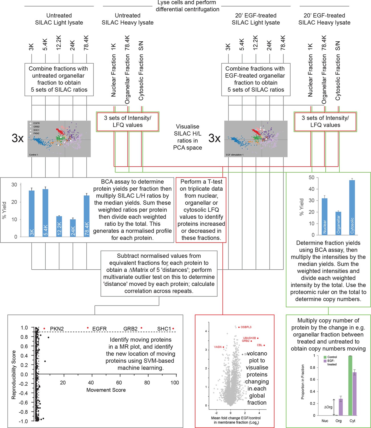
Dynamic organellar maps (EGF-treatment) – overview of the experimental workflow.
Starting with SILAC light and heavy cells in both conditions, lyse each batch of cells separately. Subject the lysates to differential centrifugation, generating membrane sub-fractions with light lysate and global fractions with heavy lysate. To identify moving proteins with precise location (follow grey lines), mix light fractions 1:1 with global membrane fraction of identically treated cells, to obtain ratios, which are visualised in PCA space. Weight SILAC L/H ratios by protein amount in the light fraction. Subtract equivalent weighted ratios of the untreated samples from the treated samples to obtain a difference profile of five differences for each protein. Repeat this three times, apply statistical test to identify moving proteins (MR plot). Use SVM-based machine learning to identify the new location of proteins that have moved. To identify proteins moving within the global membrane, nuclear and cytosolic fractions (red lines), measure the heavy fractions and quantify using MaxLFQ (Cox et al., 2014). Perform a T-test on triplicate data to reveal protein abundance changes in the global fractions. For copy number changes (green lines), multiply the intensity data by the protein yields, and use the sum of these values in the proteomic ruler (Wisniewski et al., 2014) to obtain total copy numbers. Multiply the copy numbers by the change in the proportion of a protein in a global fraction to obtain copy numbers entering or leaving this fraction.
Figure 4—figure supplement 2
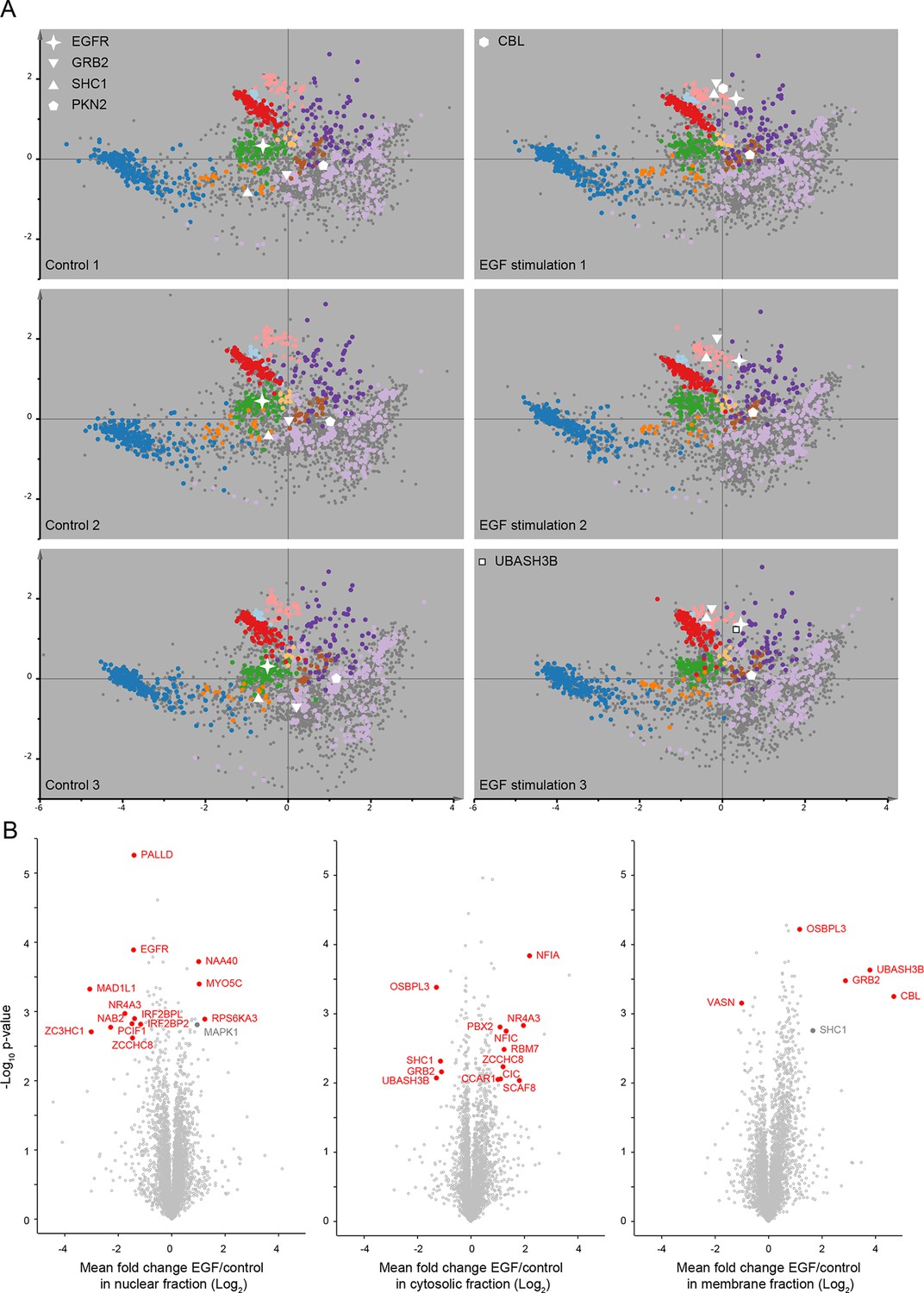
Protein localization changes following EGF stimulation.
(A) Organellar maps were prepared from untreatedHeLa cells (control, left side), and from cells following continuous stimulation with EGF for 20 min (+EGF, right side). The individual maps from triplicate biological repeats are shown, visualized by PCA. Organellar clusters are colour coded as in Figure 2. Major translocating proteins are shown as unique symbols. CBL and UBASH3B were identified in only one of the +EGF maps; they are mostly cytosolic before EGF treatment, and hence not identified in control maps. (B) Detection of EGF-induced global profile changes. Nuclear, membrane and cytosolic fractions from the experiments described in A) were subjected to mass-spectrometric analysis using label-free quantification (LFQ). Mean Log2 LFQ values from triplicate control experiments were subtracted from triplicate EGF stimulation experiments and plotted against Student’s (two-sided) t-test p-value for that difference (a ‘volcano’ plot). Proteins that increase in abundance in the relevant compartment following EGF stimulation are found on the right-hand side of the plots. Proteins undergoing significant translocations are shown in red, based on cut-offs determined as follows. First, the protein must show a minimum two-fold change in abundance (absolute log-difference >1). Second, the protein must constitute at least 10% of the total pool, either before or after EGF stimulation, in the compartment where it is shown to be changing (as determined from the protein’s global intensity profile; see Figure 1A). Finally, the p-value cut-off was FDR-controlled using the six control maps generated in Figure 2—figure supplement 2A as a mock experiment, in which no true positives would be expected. Three maps were assigned as mock-treated, three as control. For each compartment, a p-value cut-off was chosen such that no false positives would be detected in the mock experiment, but changes could still be detected in the genuine experiment (FDR = 0). This was possible for cytosolic and membrane fractions (-log10 p=2.0 and 3.1, respectively). In the case of the nucleus (-log10 p=2.6), two false positives are expected among the 13 positives (FDR ≈ 15%). Two relevant changes (shown in grey) narrowly missed significance with our extremely stringent cut-offs (SHC1 in the organellar fraction, and MAPK1 in the nuclear fraction). While their p-values were sufficiently high to reach significance, their fold-changes were just below two.
Figure 4—figure supplement 3

Global protein distribution profile changes induced by EGF treatment.
For proteins undergoing significant localization changes (Figure 4—figure supplement 1, Supplementary file 7), the distribution between nuclear, organellar and cytosolic fractions is shown before and after EGF treatment (bars show mean ± SD, n=3). Many proteins show transitions between nuclear and cytosolic fractions (eg CIC, NAA40). Several are recruited to the organellar fraction, from the cytosolic pool (eg CBL, GRB2, and SHC1). VASN shows overall degradation. Please refer to the Methods for full details on the interpretation of global distribution profiles and their changes. Furthermore, note that in each case, the three control fractions are normalized to a sum of 1. If EGF treatment changes the overall abundance of a protein, the sum of the three +EGF fractions will be different from 1 (eg <1, if the protein is degraded).
Figure 5
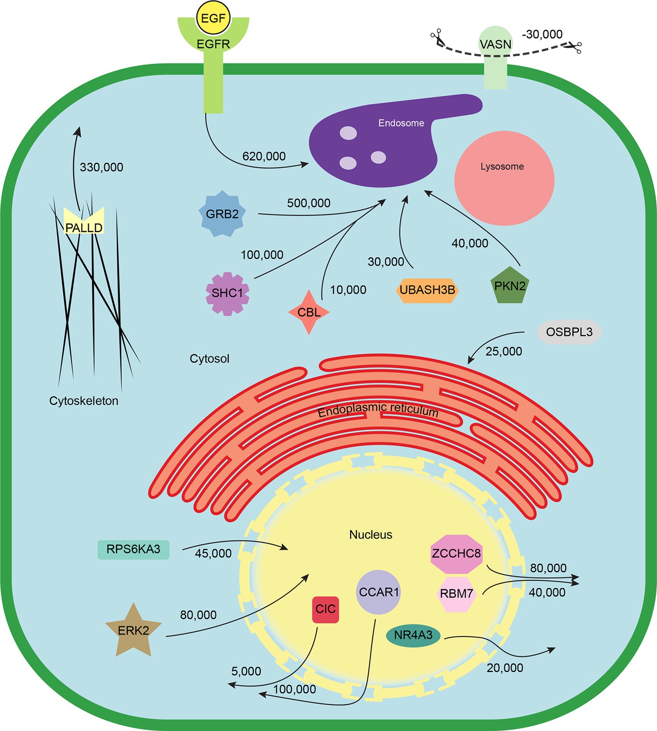
Quantitative mapping of EGF-triggered subcellular translocation events.
Summary of key protein translocations in HeLa cells following 20 min of continuous stimulation with EGF. All depicted changes were detected by organellar maps in this study; they include numerous previously known as well as novel translocation events. Numbers on arrows indicate how many copies of a protein undergo the indicated movement (per cell). These estimates were also calculated from the mass spectrometry data, using the proteomic ruler approach (Wisniewski et al., 2014). Figure 4—figure supplement 3 and Supplementary file 6 (interactive database) and 7 (compact summary) show additional translocations not included here.
Tables
Table 1
Prediction output and performance of HeLa organellar maps. The table shows the combined organellar prediction output from six replicate maps from HeLa cells. Prediction performance is judged by the proportion of correctly assigned organellar marker proteins. Please also refer to Supplementary file 1 (compact format) and 4 (complete database), which contain detailed information for all 8710 proteins covered in this study, including nuclear and cytosolic predictions. Supplementary file 2 shows the performance of each individual map.
| Compartment | Number of marker proteins | Correctly predicted markers | All proteins predicted in this compartment | |
|---|---|---|---|---|
| Number | % | |||
| Endosome | 85 | 75 | 88.2% | 304 |
| ER | 127 | 127 | 100.0% | 530 |
| ER, high curvature | 11 | 11 | 100.0% | 45 |
| ERGIC/cisGolgi | 26 | 25 | 96.2% | 73 |
| Golgi | 33 | 29 | 87.9% | 190 |
| Lysosome | 43 | 41 | 95.3% | 88 |
| Mitochondrion | 242 | 239 | 98.8% | 658 |
| Peroxisome | 21 | 15 | 71.4% | 25 |
| Plasma membrane | 127 | 123 | 96.9% | 510 |
| All organellar proteins | 715 | 685 | 95.8% | 2423 |
| Average per organelle | 92.7% | |||
| Large Protein Complexes | 361 | 353 | 97.8% | 2739 |
| Total | 1076 | 1038 | 96.5% | 5162 |
Additional files
-
Supplementary file 1
The HeLa spatial proteome.
A compact summary of organellar assignments and abundance information. Also includes the organellar markers used for classification.
- https://doi.org/10.7554/eLife.16950.015
-
Supplementary file 2
Prediction performance.
The performance and depth of all 12 maps reported in this study.
- https://doi.org/10.7554/eLife.16950.016
-
Supplementary file 3
External validation of predictions.
Contains the concordance analysis with external protein subcellular localization information. Our predictions are compared to UniProt annotations, and to a mouse cell line spatial proteome.
- https://doi.org/10.7554/eLife.16950.017
-
Supplementary file 4
The complete HeLa protein subcellular localization database.
An interactive database containing the full spatial information generated in this study, including localization, copy numbers, and neighbourhood analysis.
- https://doi.org/10.7554/eLife.16950.018
-
Supplementary file 5
Anatomy of major organelles.
The quantitative composition of three major compartments, ER, mitochondria, and plasma membrane.
- https://doi.org/10.7554/eLife.16950.019
-
Supplementary file 6
EGF dynamics database.
An interactive database showing organellar predictions and abundance changes induced by EGF.
- https://doi.org/10.7554/eLife.16950.020
-
Supplementary file 7
EGF Translocation analysis.
A summary of detected organellar and nuclear/cytosolic translocation events triggered by EGF.
- https://doi.org/10.7554/eLife.16950.021
-
Supplementary file 8
Comparison of organellar profiling approaches.
An overview of the features and requirements of Dynamic Organellar Maps and the LOPIT approach.
- https://doi.org/10.7554/eLife.16950.022
-
Supplementary file 9
Raw data.
The quantitative proteomics data used in this study (SILAC, intensity and LFQ data).
- https://doi.org/10.7554/eLife.16950.023
-
Supplementary file 10
How to use www.MapOfTheCell.org.
- https://doi.org/10.7554/eLife.16950.024
Download links
A two-part list of links to download the article, or parts of the article, in various formats.
Downloads (link to download the article as PDF)
Open citations (links to open the citations from this article in various online reference manager services)
Cite this article (links to download the citations from this article in formats compatible with various reference manager tools)
Global, quantitative and dynamic mapping of protein subcellular localization
eLife 5:e16950.
https://doi.org/10.7554/eLife.16950


