Automated structure refinement of macromolecular assemblies from cryo-EM maps using Rosetta
- University of Washington, United States
- University of California, San Francisco, United States
Figures
Figure 1 with 4 supplements
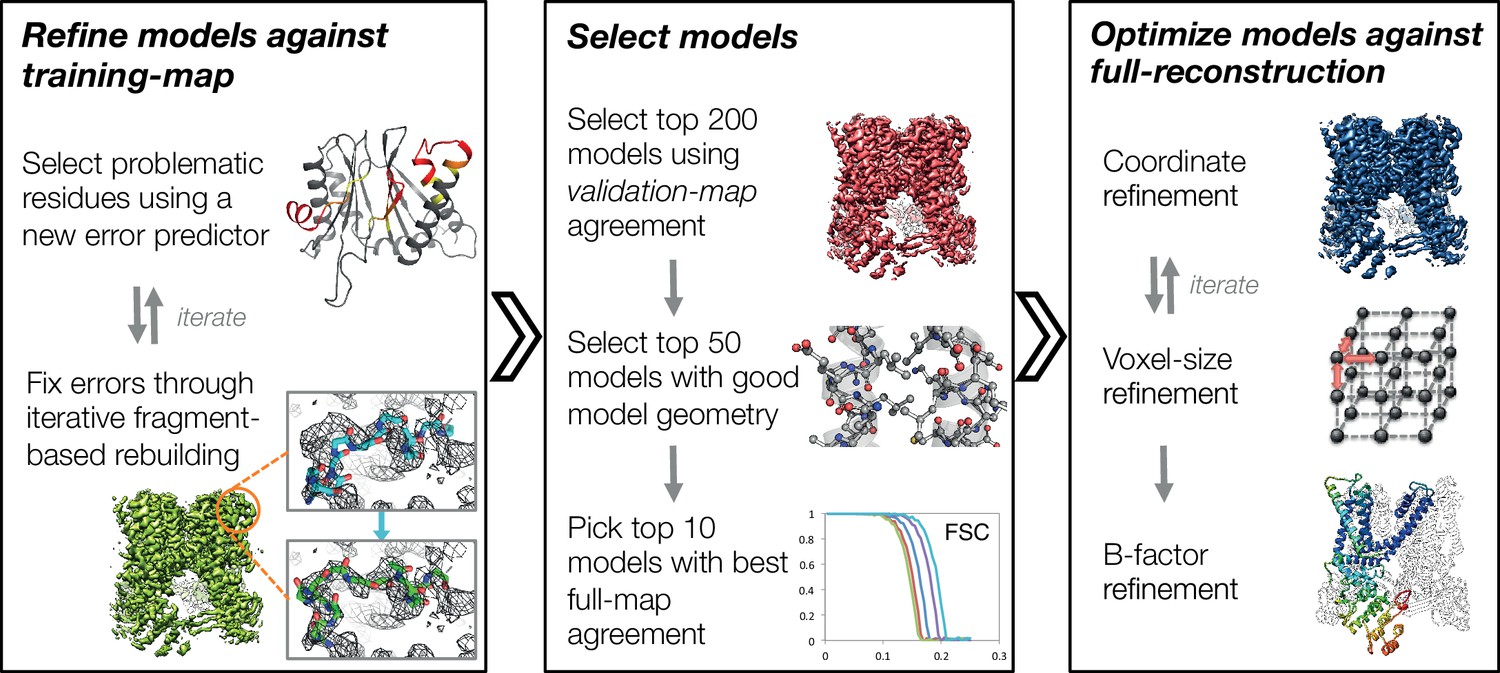
An overview of the three stages of automated refinement.
(Left) In stage 1, problematic regions are predicted using a newly developed error predictor that looks for local strain in the model and poor local density-fit. These selected regions are subject to iterative fragment-based rebuilding within a Monte Carlo sampling trajectory. Refinement in this stage is restricted to using one-half of the data, referred to as the training map. (Middle) In stage 2, the best models from the ~5000 independent Monte Carlo trajectories are selected. Models are selected based: on agreement to the validation map (independently constructed from the other half of the data), then by model geometry as assessed by MolProbity, and finally, on agreement to the full reconstruction. At this point, the selected models should in general have good fit-to-density and good geometry without overfitting to the data. (Right) In stage 3, using the 10 best models selected, we then optimize against the full reconstruction. Two half maps are used to choose the optimal density weight to refine structures using full-reconstruction. Finally, these top 10 models are optimized (without large-scale backbone rebuilding) into the full-reconstruction, which alternates with voxel-size refinement iteratively. Finally, these models are subject to B-factor refinement.
Figure 1—figure supplement 1
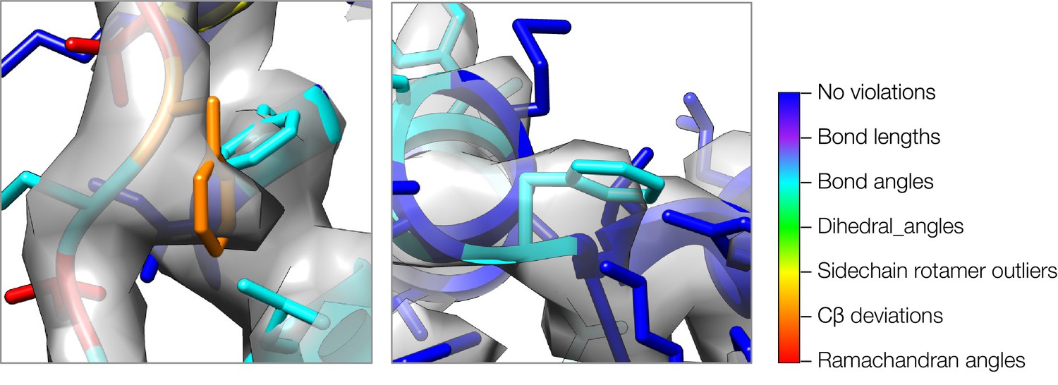
A close-up view of model strain indicating errors in density-optimized TRPV1 models using the superceded Rosetta approach.
Both insets show two regions of models refined by the superceded Rosetta approach, where strain can indicate errors in models. In both cases, phenylalanine sidechains fit the density well, but both show geometric strain around the Cβ atom. The type of strain (as evaluated by MolProbity) is indicated by model color, using the key on the right.
Figure 1—figure supplement 2
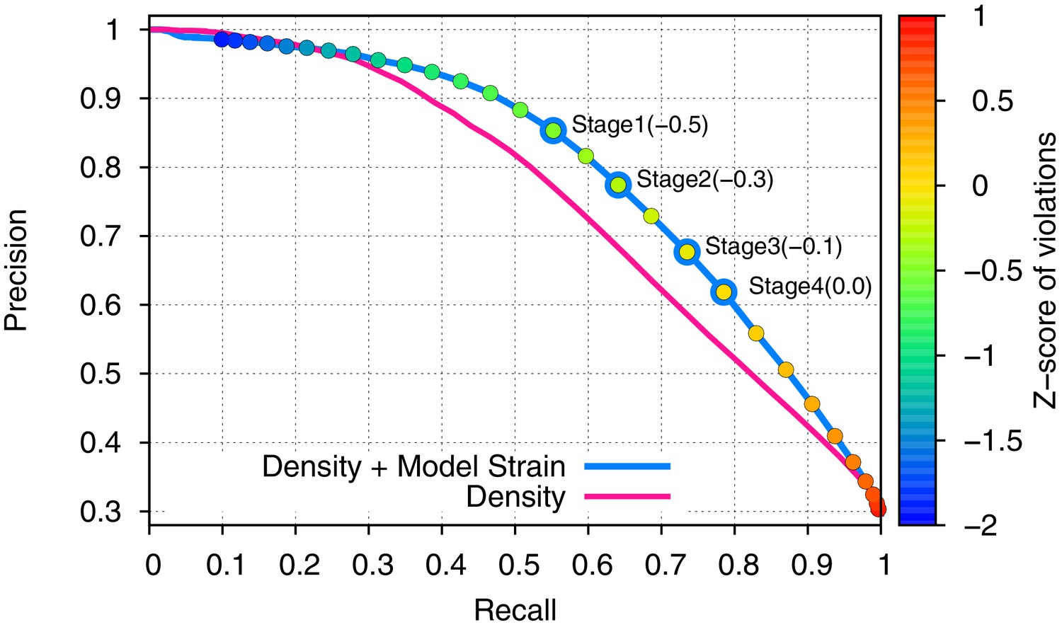
Incorporating model strain improves error detection.
Guided by the 3.3-Å 20S proteasome reconstruction, we evaluated 500 models against the high-resolution crystal structure. We plot here the precision (y-axis) and recall (x-axis) of predicting which residues were incorrectly placed (RMS > 1Å). Use of density alone (pink line) is outperformed by using a combination of density and model strain (blue line). Our refinement approach considers four points on this curve when picking density + model strain cutoffs, indicated on the plot with 'Stage1–4'.
Figure 1—figure supplement 3
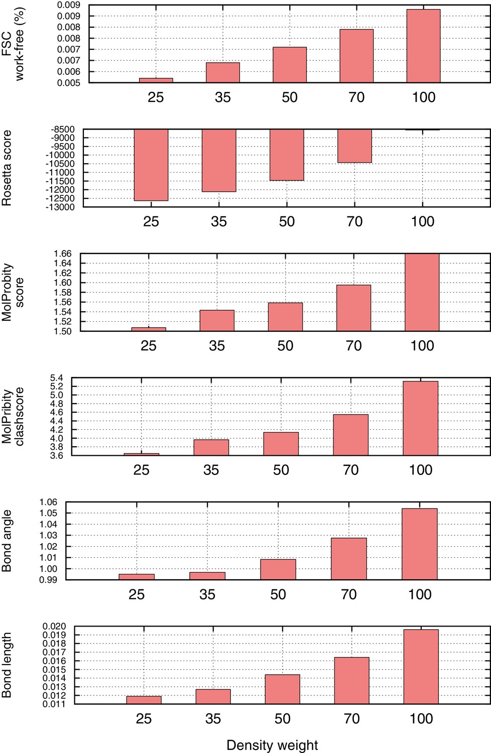
Density weight optimization against half maps for Mitoribosome.
Before refinement against the full reconstruction, we optimize the weight on the 'fit-to-density' energy using half maps, to avoid overfitting. We plot several key metrics here as a function of weight on the fit-to-density score term (x-axis), including the Fourier Shell Correlation (FSC) 'overfitting' (FSC work-free, top histogram), the Rosetta energy (second histogram), and several Molprobity model geometry terms (histograms 3–6). In all cases, we see a sharp inflection point at which overfitting increases and geometry gets notably worse. As a general rule-of-thumb, we use the weight maximizing FSCfree–(0.04*per-residue-energy to capture this inflection point).
Figure 1—figure supplement 4
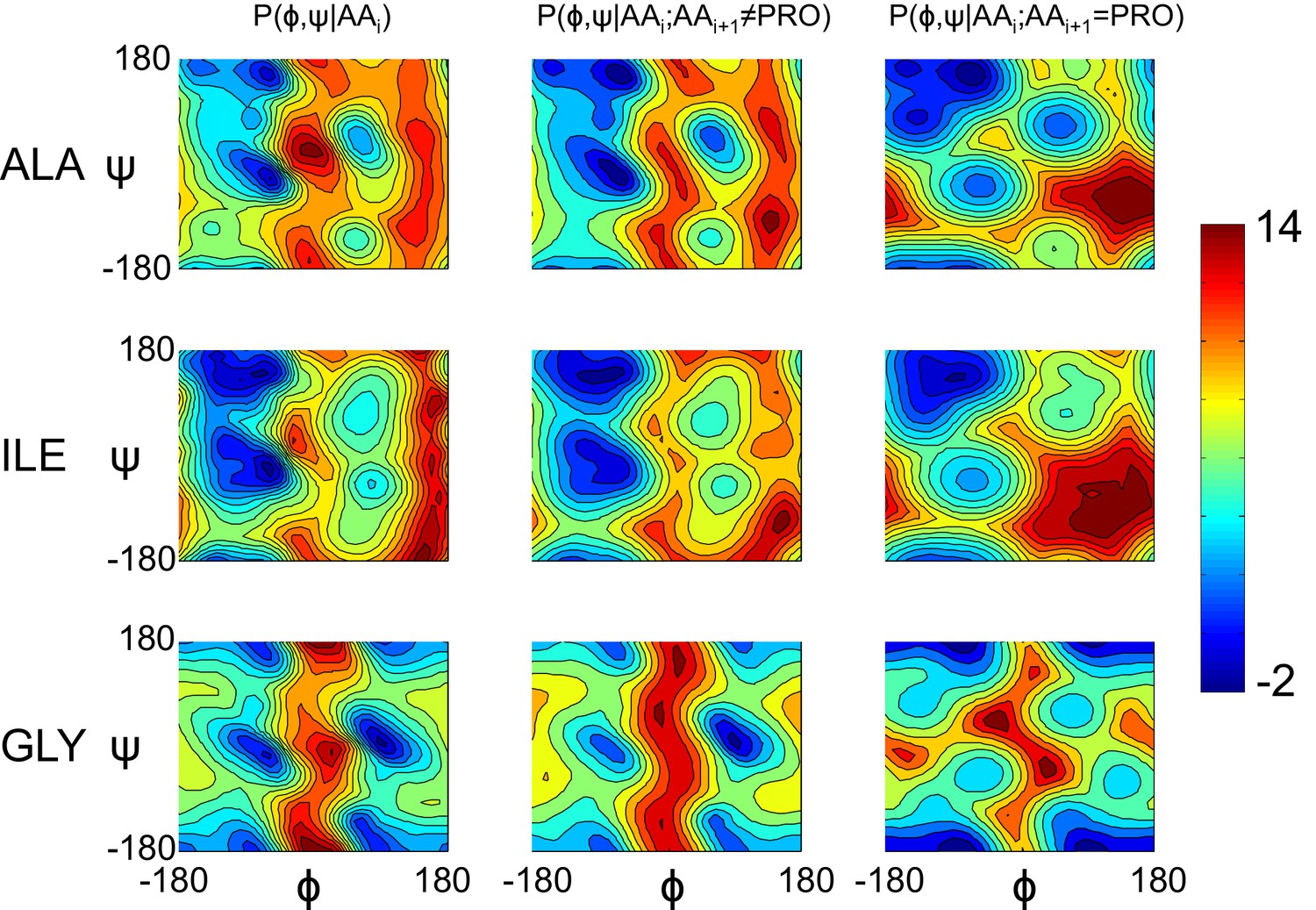
Model geometry is improved with a separate pre-proline potential.
Refined models initially had poor pre-proline geometry. Thus, a new backbone torsional potential was created which separately treats pre-proline and pre-non-proline residues. In the plot, we show the old potential (left), the new pre-non-proline potential (middle), and the pre-proline potential (right) for three different residue identities. The color indicates the unweighted energy values, using the key on the right.
Figure 2
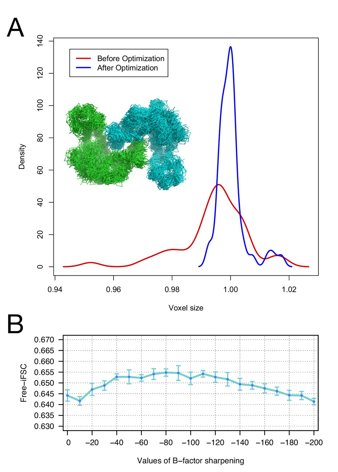
The accuracy of voxel size refinement and the effect of B-factor sharpening in Rosetta refinement.
(A) Voxel-size refinement on perturbed models. Perturbed structures were generated by running short MD trajectories in Rosetta, followed by all-atom minimization. Voxel size is refined against the perturbed models, yielding the density distribution in red. Following cycles of iterated voxel refinement and all-atom refinement, the voxel size shows significantly better convergence (blue line). (B) Rosetta structure refinement with a range values of B-factor sharpening. Integrated Fourier Shell Correlation eavluated using the validation map (free-iFSC) is plotted here as a function of B-factor sharpening of the training map. The results indicate that our refinement method is not particularly sensitive to the extent of B-factor sharpening, behaving similarly over a range of sharpening values between −40 and −130. The error bars show standard deviation of the free-iFSC among the top10 ensemble models (see Materials and methods for the ensemble selection method).
Figure 3

Refinement of the apo TRPV1 channel (EMD-5778) shows improved model quality.
(A) Comparison of the deposited and Rosetta-refined models, as assessed by MolProbity. Residues reported as violations are colored using the key shown on the far right. Blue open arrows indicate that the hydrogen-bond geometry of a β-hairpin was automatically detected and improved in the Rosetta refined model. (B) An overlay of the asymmetric unit of the deposited (pink) and the Rosetta-refined (green) model indicates the magnitude of conformational changes that are explored by our refinement approach. (C) The agreement of models to map assessed by Fourier space correlation (y-axis) at each resolution shell (x-axis), where the reported resolution (3.4Å) is depicted in a dashed orange line.
Figure 4
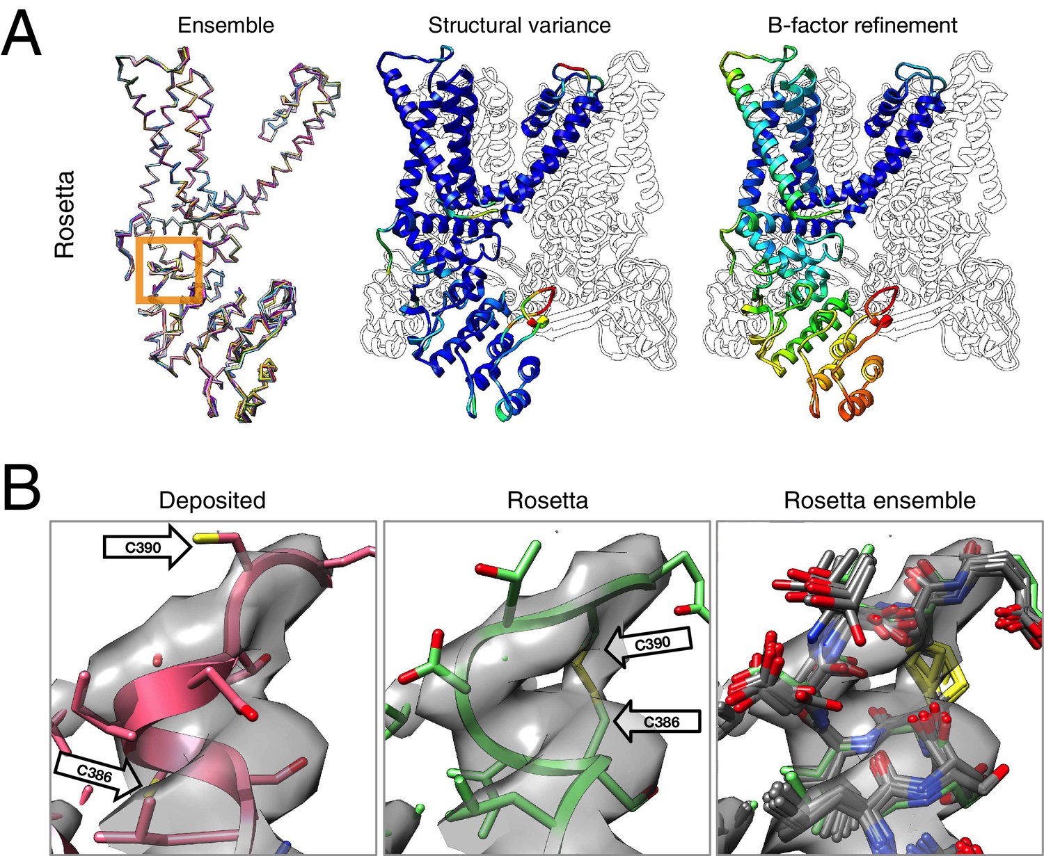
Refinement of the TRPV1 channel identifies a previously unmodeled disulfide bond.
(A) An overview of the entire structure, estimating local model uncertainty in two ways: local structural diversity and refined B-factors. Local structure diversity is indicated by showing (left) an overlay of the top 10 Rosetta models, (middle) the top model colored by per residue deviation, and (right) the refined per-atom B-factors. Using the model selection method illustrated in the middle panel of Figure 1, the Cα RMSDs among the selected ensemble range from 0.44 to 0.63 Å. The orange square shows the location of a newly identified disulfide bond (C386–C390) revealed by our refinement protocol. (B) A zoomed-in view of the disulfide linkage (C386–C390) identified by the automated method. Note that the sidechain coordinates of C390 were unassigned in the deposited model; for presentation, the sidechain atoms of C390 were optimally added by Rosetta on the basis of the deposited backbone torsion angles of C390.
Figure 5 with 1 supplement
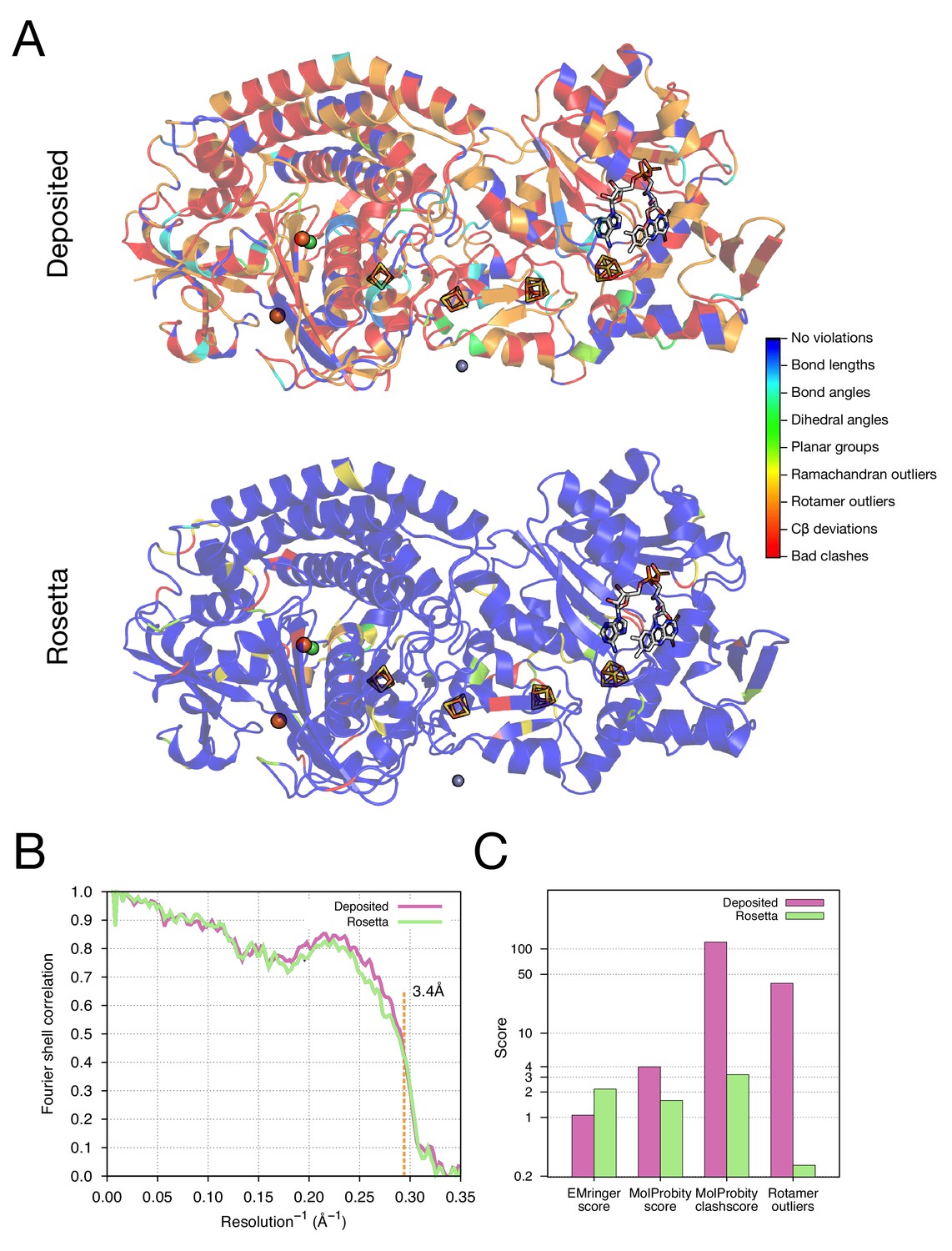
Refinement of the F420-reducing [NiFe] hydrogenase (EMD-2513) improves the model geometry.
(A) An illustration comparing the model geometry of the deposited (upper panel) and Rosetta-refined (lower panel) models. Three chains (A/B/C) of the asymmetric unit of the complex are shown as cartoon with geometry violations reported by MolProbity colored according to the key shown on the far right. Four iron–sulfur clusters [4Fe4S] and a FAD are shown in a stick representation. Metal ions are depicted as spheres, with Zn grey, Fe orange, and Ni green. (B) Model–map agreement – as assessed by Fourier shell correlation (y-axis) as a function of resolution (x-axis) – quantifies this improvement following voxel-size refinement. (C) Model quality as assessed by EMRinger and MolProbity. The x-axis shows methods used to evaluate the models, while the y-axis shows the scores under each criterion.
Figure 5—figure supplement 1

The symmetry operators denoted in the deposited PDB (PDB 4ci0) produce a complex that could not fit into the deposited density map properly.
(Left panel) The symmetric complex downloaded from a protein data bank as a biounit shifts the entire complex out of the deposited density map. The middle and right panels show a zoomed-in view of two regions in the deposited models corresponding to the helix and the sheet indicated by the orange and cyan squares, respectively, in the left panel.
Figure 6 with 2 supplements
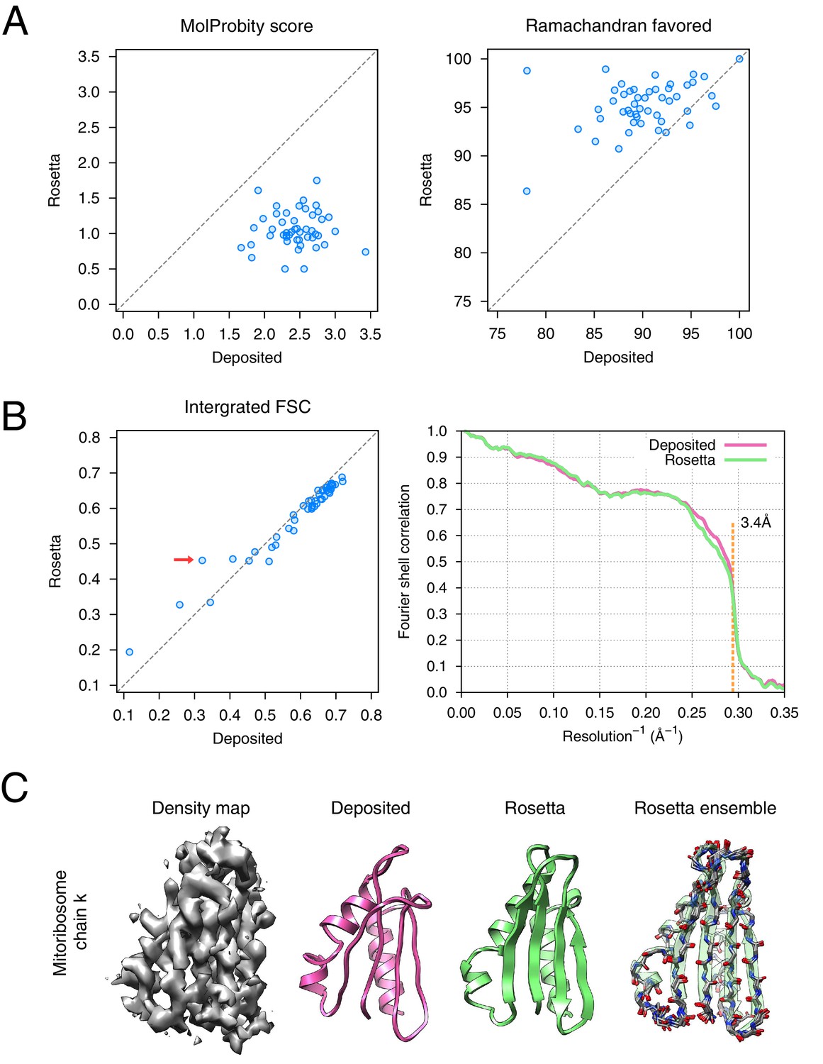
Refinement of the large subunit of the human mitochondrial ribosome (EMD-2762) shows improvements to all subunits.
(A) Scatterplots of model quality for each of the 48 protein chains compare the deposited (x-axis) and Rosetta (y-axis) models using MolProbity. On the left, the MolProbity scores of all 48 protein chains are compared, where a lower values indicates a better model geometry. On the right, the percentage of 'Ramachandran favored' residues on each chain are compared, with higher values preferable. (B) An evaluation of the fit-to-density of each protein chain. On the left, we compare the Fourier shell correlation (FSC) of each chain before and after refinement; we integrate the FSC from 10Å to 3.4Å. Higher values indicate better agreement with the data. The largest improvement, chain k, is indicated by the red arrow. On the right, we show the full FSC curve, with the deposited model shown in pink, and the Rosetta refined model shown in green; the reported map resolution (3.4Å) is indicated in the dashed orange line. (C) A zoomed-in view indicating a much improved backbone geometry and the large radius of convergence of the refinement of chain k. The left panel shows that the density for chain k is in the region of relatively low local resolution.
-
Figure 6—source data 1
Mitoribosome per-chain refinement results.
- https://doi.org/10.7554/eLife.17219.014
Figure 6—figure supplement 1
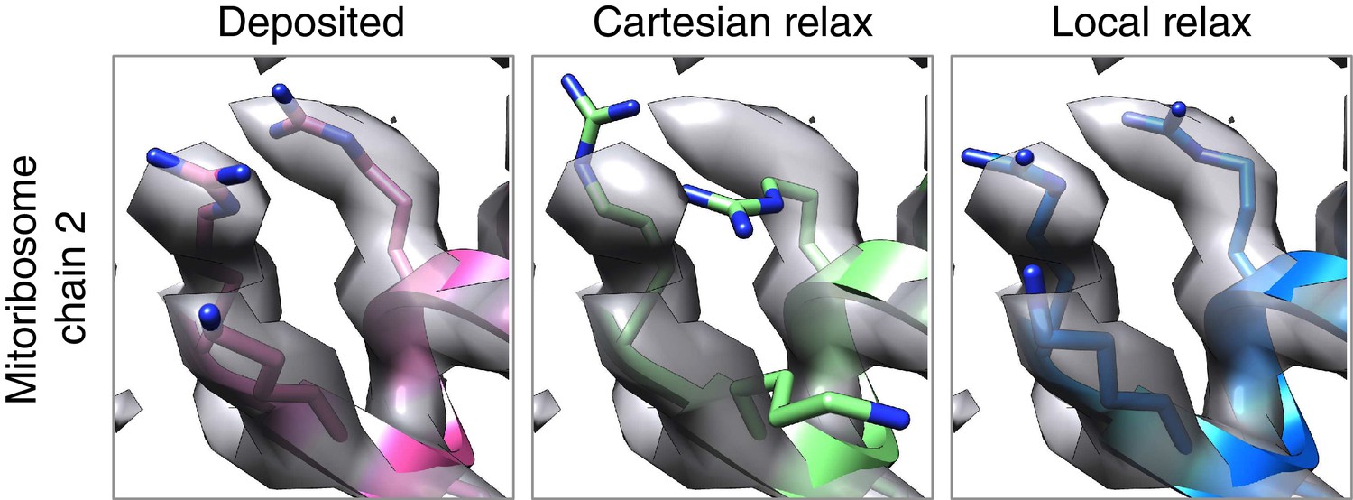
Local relax shows better placement of sidechains for large systems.
In the case of the mitoribosome, refinement of a particularly well-resolved region in the map (left) led to sidechains that are clearly misaligned with the density (middle). This was due to the poor convergence of our Monte Carlo sidechain placing approach when applied to systems with more than 1000 residues. Our alternative approach, LocalRelax, which performs many local sidechain optimizations, correctly places sidechains in a way that is consistent with density (right).
Figure 6—figure supplement 2
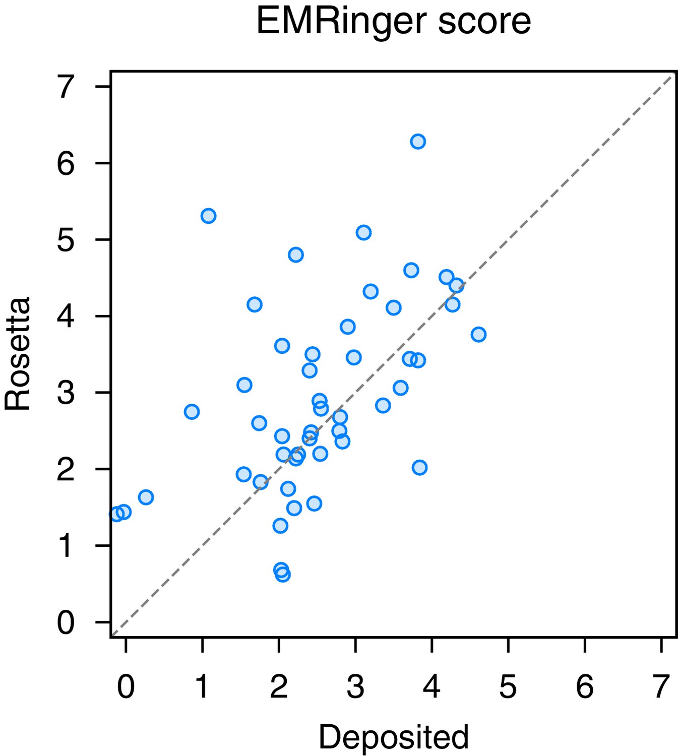
EMRinger analysis on refinement of the large subunit of the human mitochondrial ribosome.
A scatterplot of model quality assessed by EMringer of each of the 48 protein chains compares the deposited (x-axis) and Rosetta (y-axis) models.
Tables
Table 1
Structure refinement of macromolecular assemblies from cryo-EM maps using Rosetta.
| EMD ID | PDB ID | Reported resolution [Å] | Symmetry | Number of amino acids* | MolProbity† | EMRinger score† | iFSC‡ | ||||
|---|---|---|---|---|---|---|---|---|---|---|---|
| Score | Clash score | Rotamer outliers [%] | Ramachandran favored [%] | ||||||||
| TRPV1 | 5778 | 3j5p | 3.4 | C4 | 489 (1956) | 3.81 / 1.45 | 86.35 / 1.96 | 28.78 / 0.00 | 95.65 / 91.93 | 0.65 / 2.34 | 0.612 / 0.607 |
| Frh | 2513 | 4ci0 | 3.4 | T | 893 (10,716)§ | 3.98 / 1.59 | 120.42 / 3.22 | 39.11 / 0.27 | 96.51 / 92.18 | 1.06 / 2.17 | 0.743 / 0.708 |
| Mitoribosome | 2762 | 3j7y | 3.4 | N/A | 7469¶ | 2.71 / 1.50 | 8.38 / 3.51 | 8.49 / 0.08 | 89.86 / 94.86 | 2.09 / 2.40 | 0.692 / 0.676 |
-
*Number of protein residues in the asymmetric unit and (the total residues) modeled.
-
†Scores from deposited (left) versus (/) Rosetta refined (right) model.
-
‡Integrated Fourier Shell Correlation (iFSC) from 10–3.4Å resolution shells.
-
§In addition to protein residues, nine residues of ligand per asymmetric unit–including a [NiFe] cluster, two metal ions (Fe and Zn), and four [4Fe4S] clusters, and an FAD–were included in the refinement.
-
¶In addition to protein residues, 1529 base pairs of RNA molecule were included in the refinement.
Table 2
Comparison of structure refinement results between Rosetta and phenix.real_space_refine*.
| RSCC*,†,‡ validation map | iFSC*,†,§ validation map | EMRinger Score*,† validation map | MolProbity† | Number of residues with better RSCC†,¶ | ||||
|---|---|---|---|---|---|---|---|---|
| Score | Clash score | Rotamer outliers [%] | Ramachandran favored [%] | |||||
| TRPV1 | 0.785 / 0.790 | 0.546 / 0.566 | 1.84 / 1.90 | 1.59 / 1.48 | 4.30 / 2.14 | 0.00 / 0.00 | 94.41 / 91.72 | 86 / 250 |
| Frh | 0.835 / 0.835 | 0.504 / 0.517 | 1.36 / 1.27 | 1.68 / 1.62 | 7.99 / 3.66 | 0.68 / 0.13 | 96.31 / 92.67 | 677 / 1328 |
| Mitoribosome | 0.832 / 0.832 | 0.476 / 0.478 | 2.05 / 1.98 | 1.88 / 1.62 | 6.17 / 4.08 | 0.38 / 0.00 | 90.19 / 93.49 | 415 / 564 |
-
*To avoid over-fitting, refinement using both methods was carried out using the half-map approach, in which the models were subject to refinement using the training maps. The results showing here were evaluated using the validation-maps. The input model information is the same as reported at Table 1.
-
†Numbers (scores) from phenix.real_space_refine (left) versus (/) Rosetta refined (right) model.
-
‡Real-space correlation coefficients were evaluated using UCSF Chimera.
-
§Integrated Fourier shell correlation (iFSC) from 10–3.4Å resolution shells.
-
¶We calculate per-residue real-space correlation coefficient and report the number of residues which show the value of ΔRSCC greater than 0.05.
Table 3
Sidechain scaling factors used in automated Rosetta structure refinement.
| Sidechain | Raw data | Factor used |
|---|---|---|
| ARG | 0.84 | 0.66 |
| LYS | 0.84 | 0.66 |
| GLU | 0.85 | 0.66 |
| MET | 0.87 | 0.66 |
| ASP | 0.88 | 0.66 |
| CYS | 0.87 | 0.71 |
| GLN | 0.89 | 0.71 |
| HIS | 0.91 | 0.71 |
| ASN | 0.91 | 0.71 |
| THR | 0.94 | 0.71 |
| SER | 0.95 | 0.71 |
| TYR | 0.95 | 0.78 |
| TRP | 0.96 | 0.78 |
| ALA | 0.97 | 0.78 |
| PHE | 0.98 | 0.78 |
| PRO | 0.98 | 0.78 |
| ILE | 0.99 | 0.78 |
| LEU | 0.99 | 0.78 |
| VAL | 1.00 | 0.78 |
Additional files
-
Supplementary file 1
Input files to carry out the TRPV1 structure refinement described in the manuscript.
Structure refinement of TRPV1 using Rosetta involves two steps: (1) refinement of only the transmembrane regions, and (2) refinement of the full system, including the Ankyrin repeat domains. The package includes two folders, one for each of the two steps with the command lines and input files necessary to run TRPV1 structure refinement.
- https://doi.org/10.7554/eLife.17219.019
-
Supplementary file 2
Input files to carry out the Frh structure refinement described in the manuscript.
Structure refinement of Frh using Rosetta involves three steps: (1) refinement of the asymmetric unit without ligands present, (2) local refinement of the asymmetric unit with the ligands present, and (3) local refinement the full symmetric complex with ligands present. The package includes three folders, one for each of the three steps with the command lines and input files necessary to run Frh structure refinement.
- https://doi.org/10.7554/eLife.17219.020
-
Supplementary file 3
Input files to carry out the Mitoribosome structure refinement described in the manuscript.
Structure refinement of the case of Mitoribosome using Rosetta involves in two steps: (1) refinement of individual chains, and (2) local refinement the whole assembly. The package includes two folders, one for each of the two steps with the command lines and input files necessary to run Mitoribosome structure refinement.
- https://doi.org/10.7554/eLife.17219.021
Download links
A two-part list of links to download the article, or parts of the article, in various formats.
Downloads (link to download the article as PDF)
Open citations (links to open the citations from this article in various online reference manager services)
Cite this article (links to download the citations from this article in formats compatible with various reference manager tools)
Automated structure refinement of macromolecular assemblies from cryo-EM maps using Rosetta
eLife 5:e17219.
https://doi.org/10.7554/eLife.17219


