Advances in X-ray free electron laser (XFEL) diffraction data processing applied to the crystal structure of the synaptotagmin-1 / SNARE complex
- Stanford University, United States
- Lawrence Berkeley National Laboratory, United States
- SLAC National Accelerator Laboratory, United States
- University of California, San Francisco, United States
Figures
Figure 1 with 2 supplements
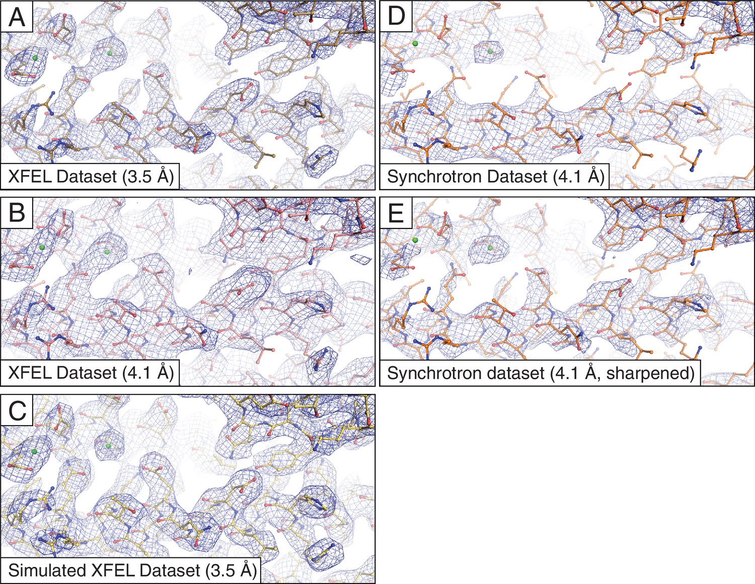
Representative 2mFo-DFc electron density maps.
The maps were obtained using (A) the XFEL diffraction data at 3.5 Å resolution; (B) same as (A) but truncated to 4.1 Å resolution in order to match the limiting resolution of the synchrotron data; (C) the simulated XFEL diffraction data set; (D) the synchrotron data set (at 4.1 Å resolution), (E) same as (D) but with the synchrotron data sharpened with Bsharp = −23 Å2 in order to account for the differences in overall B-factors of the corresponding diffraction data sets. All maps were rendered at a contour level of 2.0 σ.
Figure 1—figure supplement 1

Representative 2mFo-DFc electron density maps of an interface between the C2A and C2B domains of synaptotagmin-1.
The maps were obtained using (A) the 3.5 Å XFEL diffraction data as originally published in (Zhou et al., 2015), (B) the reprocessed 3.5 Å XFEL diffraction data and (C) the 4.1 Å synchrotron data. Note that in (C) the salt bridge between R233 and E346 could not be accurately modeled due to poor density. The map in (B) was sharpened with Bsharp = −33 Å2, and the map in (C) was sharpened with Bsharp = −23 Å2 in order to account for the differences in overall B-factors of the corresponding diffraction data sets. All maps were rendered at a contour level of 1.5 σ.
Figure 1—figure supplement 2
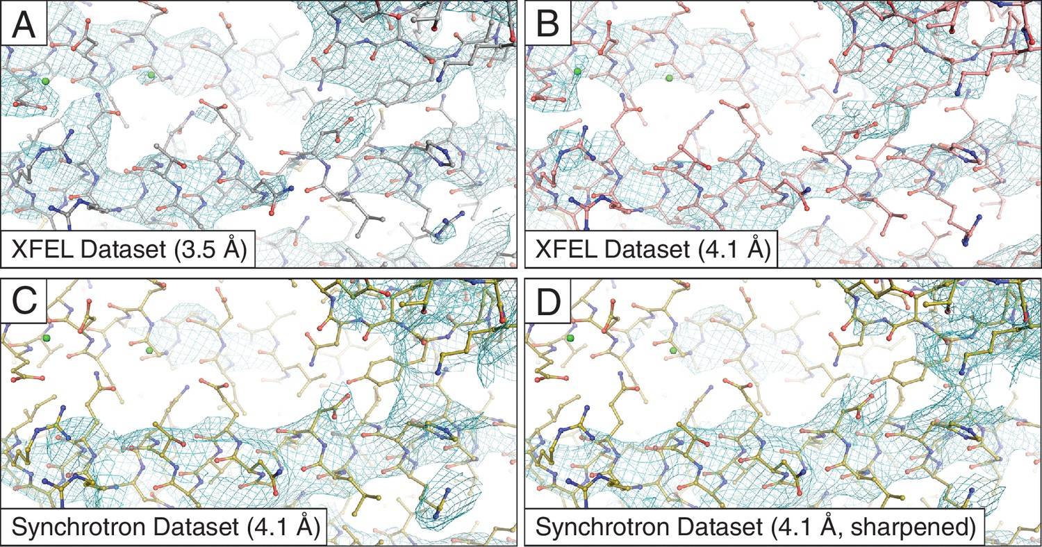
Simulated annealing composite omit maps generated using 2mFo-DFc coefficients.
The maps were obtained using (A) the 3.5 Å XFEL diffraction data; (B) same as (C) but truncated to 4.1 Å resolution in order to match the limiting resolution of (A); (C) the 4.1 Å synchrotron data set and (D) same as (C) but with the synchrotron data set sharpened with Bsharp = −23 Å2 in order to account for the differences in overall B-factors of the corresponding diffraction data sets. All maps were rendered at a contour level of 1.5 σ.
Figure 2 with 1 supplement
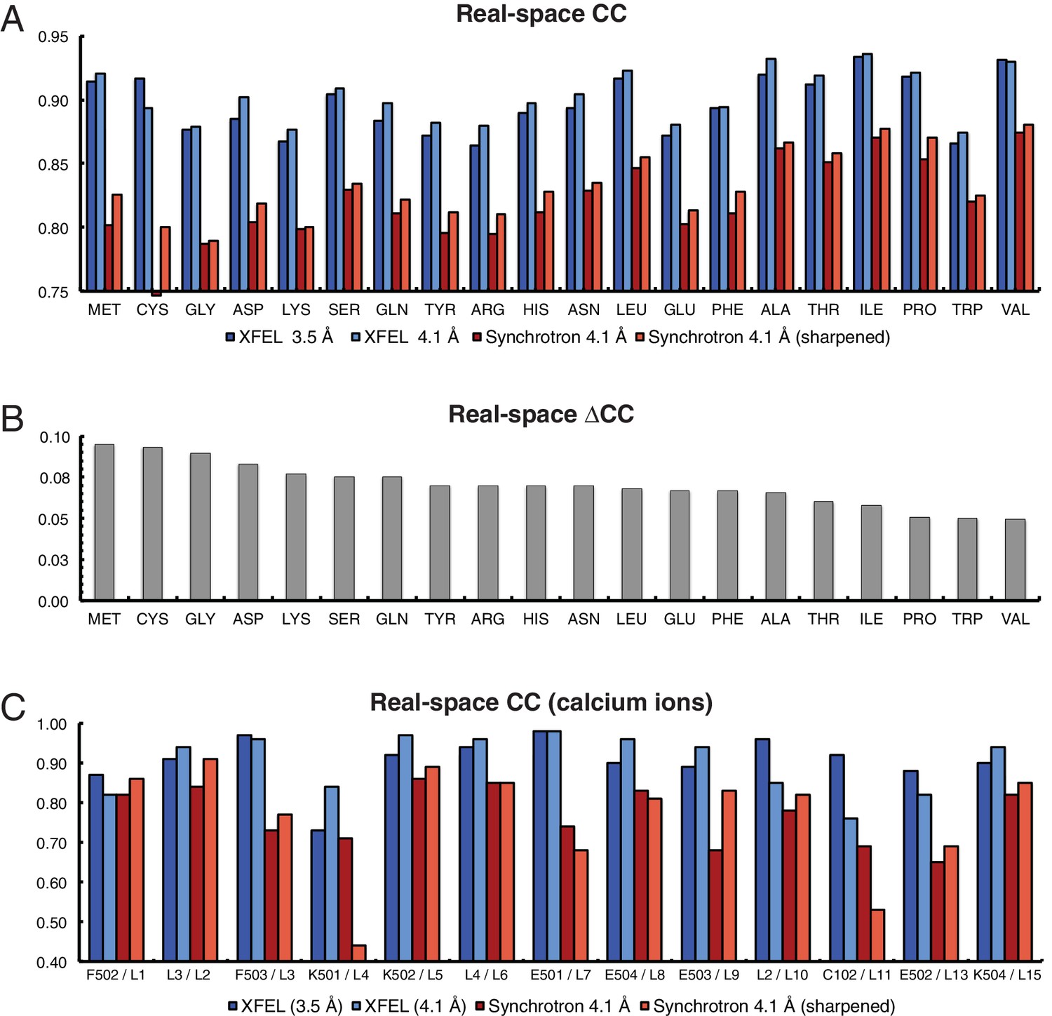
Analysis of real-space correlation for atomic models refined against the XFEL and synchrotron data sets.
(A) Real-space correlation coefficients for atomic models of the Syt1–SNARE complex refined against the XFEL (XFEL 3.5 Å, XFEL 4.1 Å) and synchrotron [Synchrotron 4.1 Å, Synchrotron 4.1 Å (sharpened)] diffraction data and analyzed by amino acid residue type; (B) differences between real-space correlation coefficients of the atomic models (ΔCC) refined against the XFEL and synchrotron diffraction data of Syt1–SNARE complex, both processed and refined at 4.1 Å resolution; (C) real-space correlation coefficients for the Ca2+ sites that were visible in the XFEL- and synchrotron-data derived Syt1–SNARE crystal structures (due to the different numbering of calcium ions in XFEL- and synchrotron-derived structures, two chain and atom labels are given for each, e.g. “F502 / L1”; the first label refers to the XFEL-derived structure, while the second label refers to the synchrotron-derived structure). To facilitate the comparison, the XFEL-based correlation coefficients were calculated at a limiting resolution of 4.1 Å (matching the limiting resolution of the synchrotron data set) as well as at the actual limiting resolution of the XFEL diffraction data set (3.5 Å). Furthermore, the electron density maps obtained from the synchrotron data were sharpened with Bsharp = −23 Å2 in order to account for the difference in overall B-factors of the diffraction data sets.
Figure 2—figure supplement 1
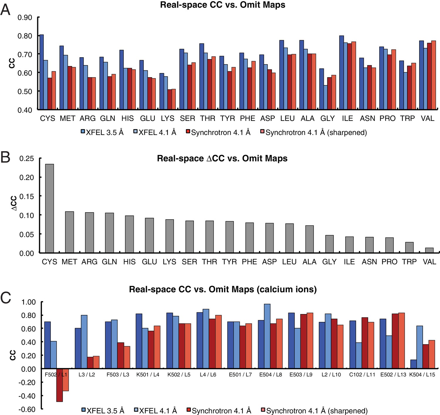
Analysis of real-space correlation for atomic models refined against the XFEL and synchrotron data sets versussimulated annealing composite omit maps.
(A) Real-space correlation coefficients for atomic models of the Syt1–SNARE complex refined against the XFEL (XFEL 3.5 Å, XFEL 4.1 Å) and synchrotron [Synchrotron 4.1 Å, Synchrotron 4.1 Å (sharpened)] diffraction data and analyzed by amino acid residue type; (B) differences between real-space correlation coefficients of the atomic models (ΔCC) refined against the XFEL and synchrotron diffraction data of Syt1–SNARE complex, both processed and refined at 4.1 Å resolution; (C) real-space correlation coefficients for the Ca2+ sites that were visible in the XFEL- and synchrotron-data derived Syt1–SNARE crystal structures. To facilitate the comparison, the XFEL-based correlation coefficients were calculated at a limiting resolution of 4.1 Å (matching the limiting resolution of the synchrotron data set) as well as at the actual limiting resolution of the XFEL diffraction data set (3.5 Å). Furthermore, the electron density maps obtained from the synchrotron data were sharpened with Bsharp = −23 Å2 in order to account for the difference in overall B-factors of the diffraction data sets.
Figure 3
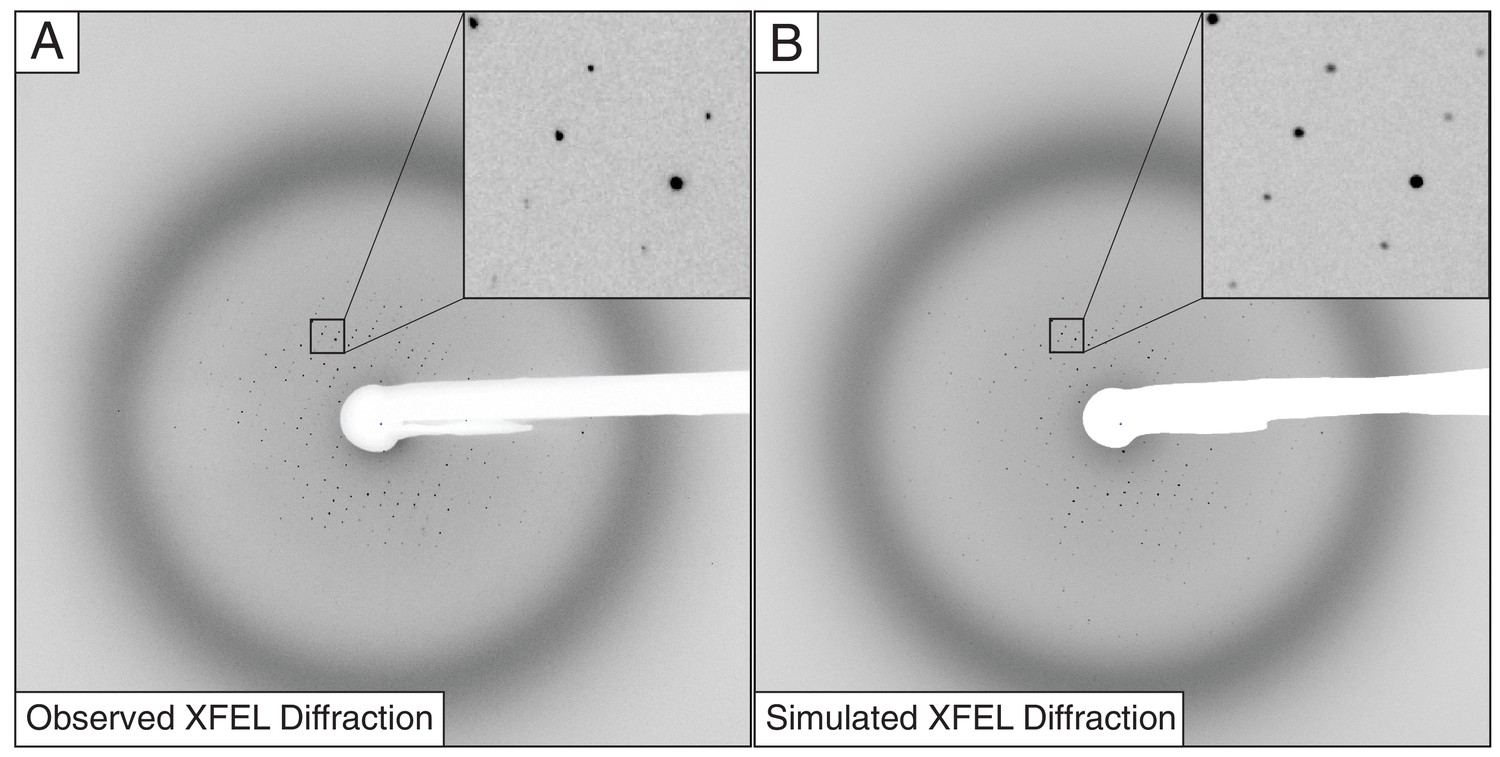
Observed (A) and simulated (B) XFEL diffraction images of the Syt1–SNARE complex.
The insets show close-up views of the indicated regions.
Figure 4 with 4 supplements
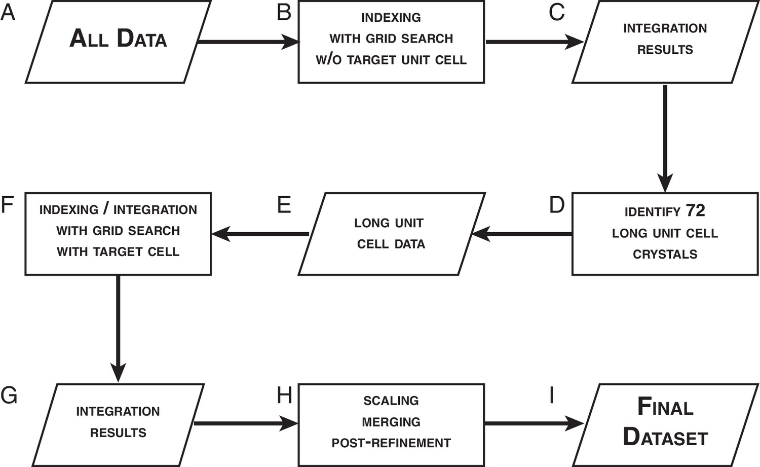
Data processing strategy for XFEL diffraction data of the Syt1–SNARE complex.
https://doi.org/10.7554/eLife.18740.010
Figure 4—figure supplement 1
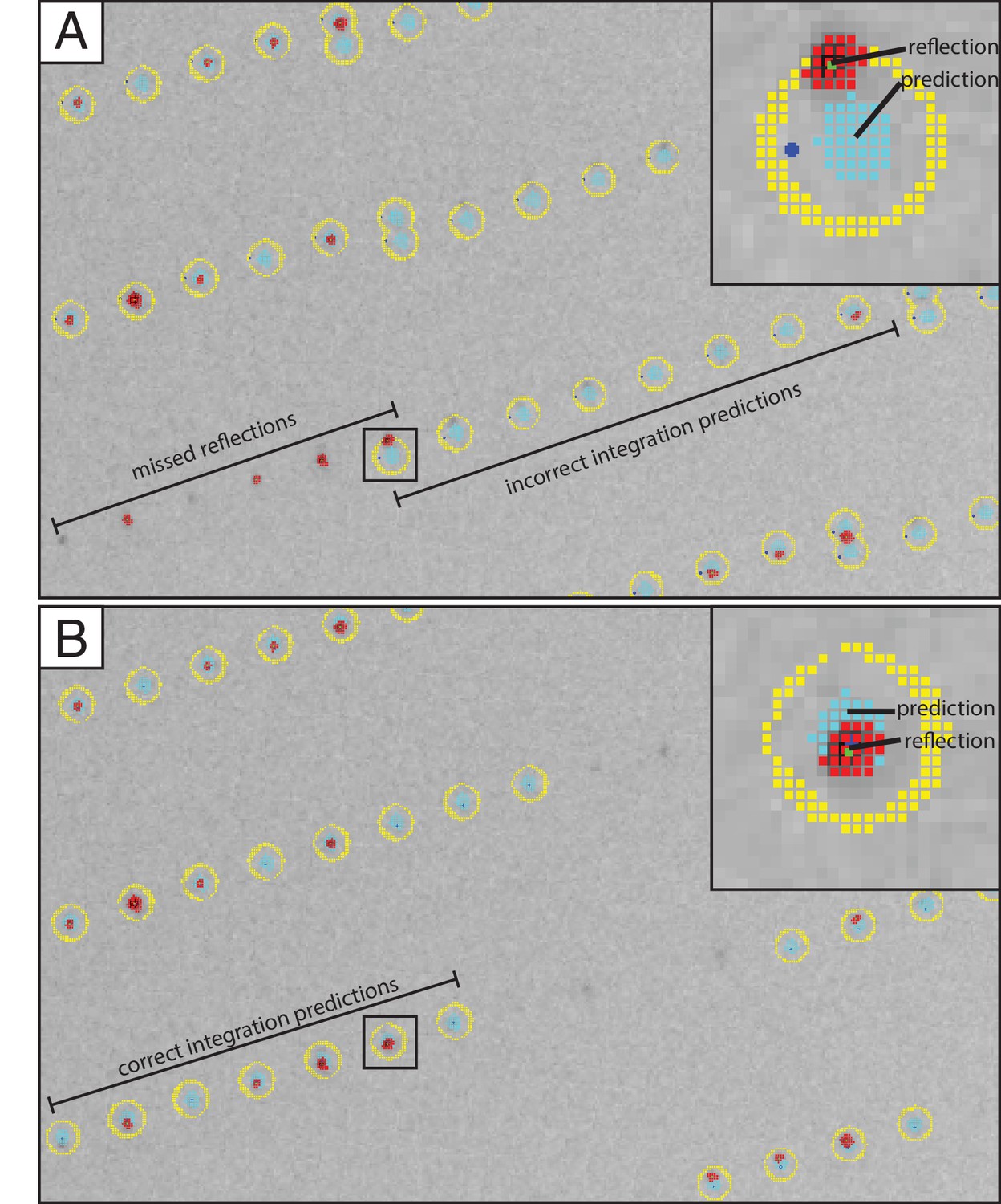
Improved crystal lattice refinement with DIALS.
Section of an XFEL diffraction image shown with overlaid integration prediction obtained with the LABELIT method implemented in cctbx.xfel (Hattne et al., 2014) and B) DIALS methods (Waterman et al., 2016) recently implemented in cctbx.xfel. A single reflection with incorrect (A, inset) and correct (B, inset) corresponding integration prediction was selected to illustrate how the new crystal lattice refinement approach implemented in DIALS results in a significant improvement of the integrated intensities. Initial spot-finding results are marked as clusters of red squares, integration masks as clusters of teal squares, and pixels used for background calculation as clusters of yellow squares.
Figure 4—figure supplement 2
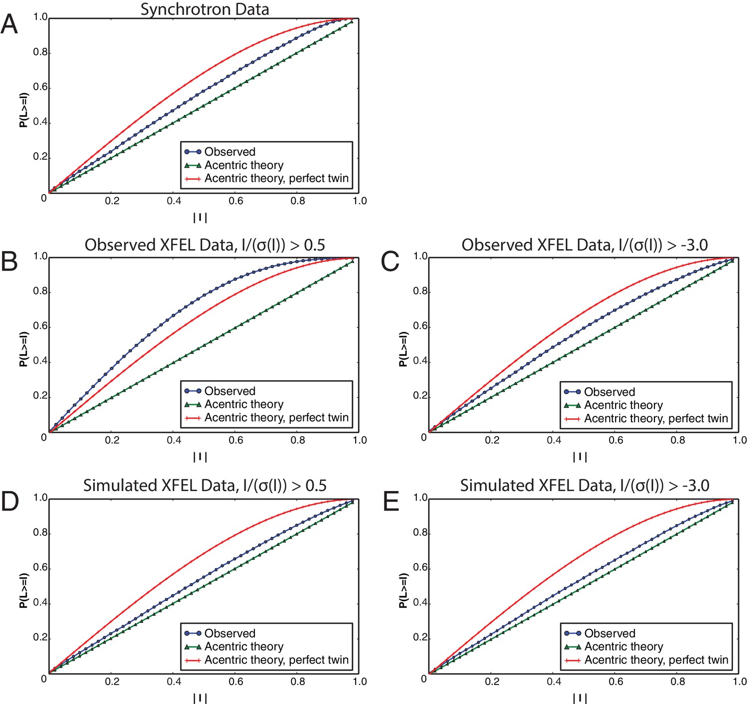
L-tests for merged diffraction data sets.
The L-tests were performed using phenix.xtriage (Zwart et al., 2005) for the (A) synchrotron data set, (B) observed XFEL data set with , (C) observed XFEL data set with , (D) simulated XFEL data set with and (E) simulated XFEL data set with . All L-tests are shown for the data sets at their respective limiting resolutions (corresponding to Table 1).
Figure 4—figure supplement 3
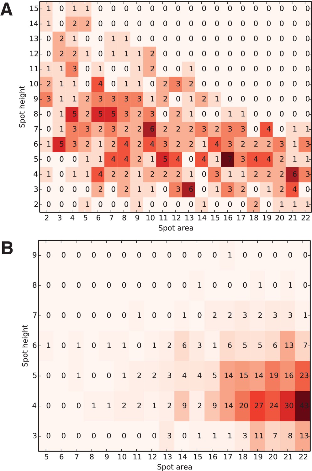
Distribution of the optimal spot-finding parameter combinations over all successfully integrated diffraction images.
Each diffraction image was indexed and integrated using every possible combination of the two spot-finding parameters; only the selected optimal integration results (one per each image) were used to construct the heat map. The color of each square represents the number of optimally integrated diffraction images (shown inside each square) for this combination of spot-finding parameters. Parameter distributions for A) experimental XFEL and B) simulated XFEL diffraction data are shown (corresponding to Table 1, columns A, C). Note the much wider distribution in experimental vs. simulated XFEL diffraction data, illustrating the image-to-image variability of serial XFEL diffraction data sets, which necessitated the grid search approach.
Figure 4—figure supplement 4
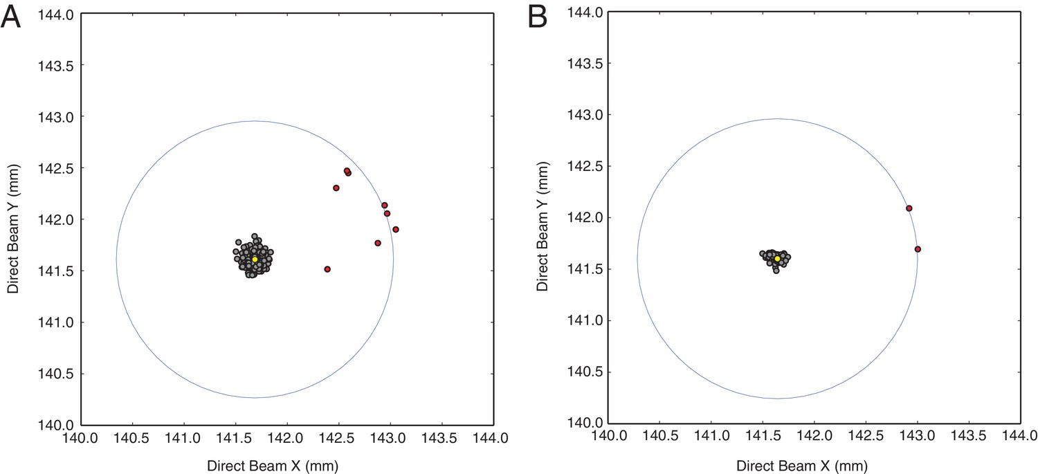
Inspection of refined direct beam coordinates indicates possible mis-indexed diffraction images.
Direct beam coordinates obtained from (A) diffraction images integrated using default direct beam coordinate refinement radius (4.0 mm) and (B) diffraction images integrated using a restricted default direct beam coordinate search area (0.5 mm). Note the bimodal distribution of direct beam coordinate sets (filled grey circles) clustered around the median (filled yellow circle) and outlier (filled red circles) clustered within a distance (~1.4 mm) approximately corresponding to the length of the c-axis (~292 Å, open blue circle), which indicates incorrect assignment of Miller indices (mis-indexing).
Figure 5 with 1 supplement
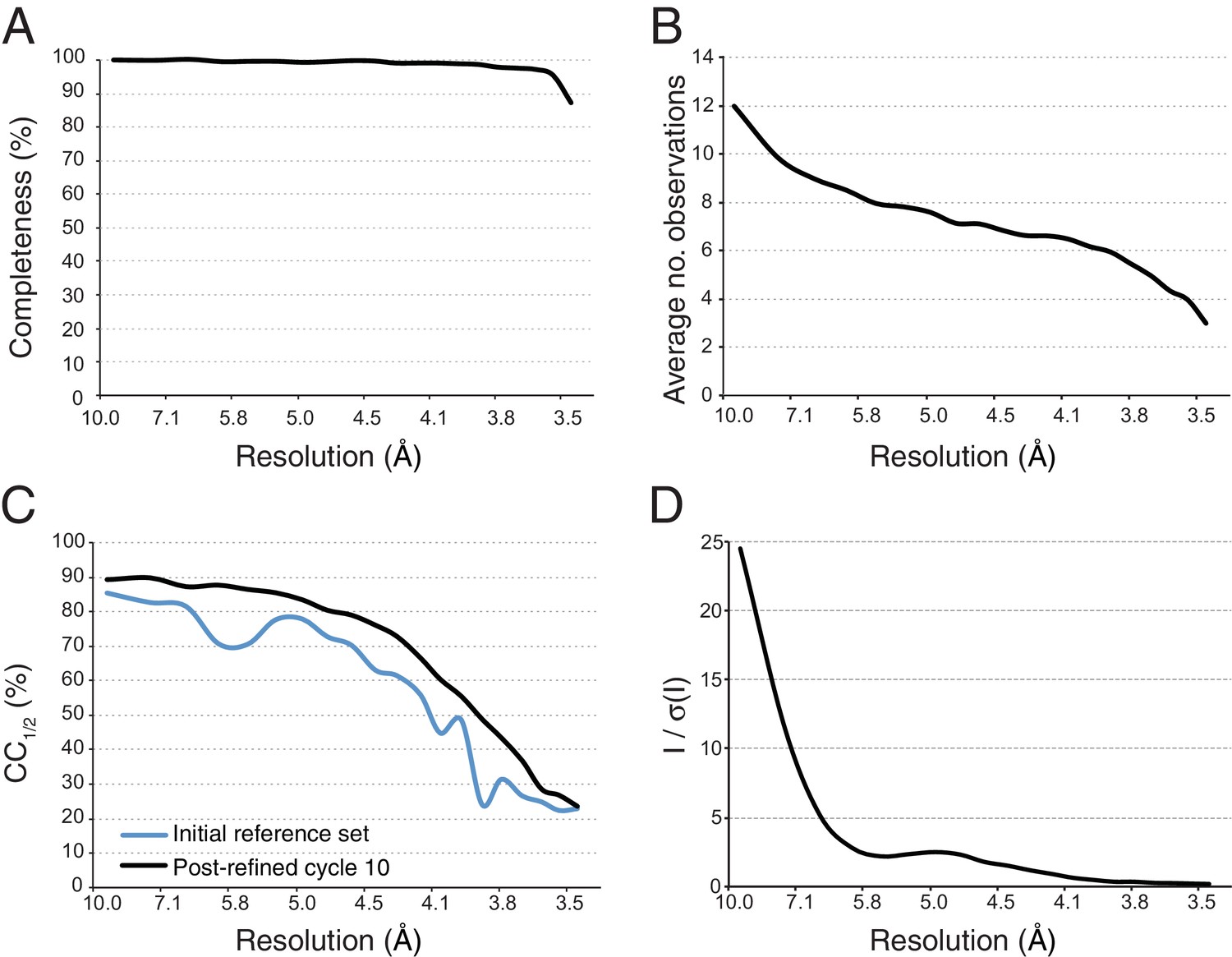
Statistical charts for scaled, merged and post-refined XFEL diffraction data.
(A) Completeness, (B) Average number of partial observations per Miller index, (C) CC1/2, comparing the initial reference set and post-refined data set, (D) I / σ(I).
Figure 5—figure supplement 1
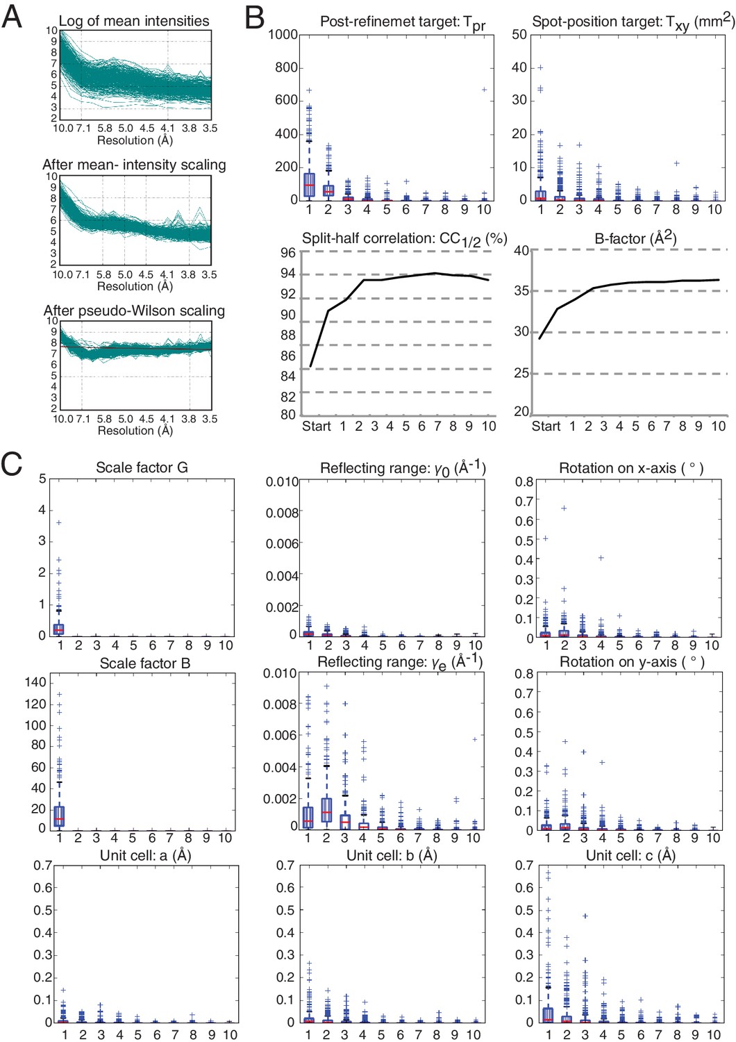
Wilson plots of the diffraction images and convergence of post-refinement after ten cycles for the XFEL diffraction data.
Changes in each parameter and target function are plotted relative to the previous cycles, while the CC1/2 metric and the B-factor are shown as absolute values for each merged data set per cycle starting from the initial reference set. The convergence of the post-refinement parameters and the refinement target functions are shown as box plots. These box plots show the first (Q1) and the third (Q3) quartiles (bottom and top of the blue box), the second quartile (Q2; red line), and the range at a 1.5 interquartile (Q3–Q1; black horizontal lines) for the particular quantity. The plus signs show any data points beyond this range. (A) Overlay of Wilson plots (on a logarithmic scale) for the observed intensities for all diffraction images (top), after mean-intensity scaling, as defined in (Uervirojnangkoorn et al., 2015) (middle), and after pseudo-Wilson scaling (bottom). (B) Convergence of post-refinement and spot-location target functions, the CC1/2 metric, and the overall B-factor of the merged data. (C) Convergence behavior of the all post-refined parameters. In all plots in (B) and (C), the horizontal axis is the post-refinement cycle number.
Author response image 1
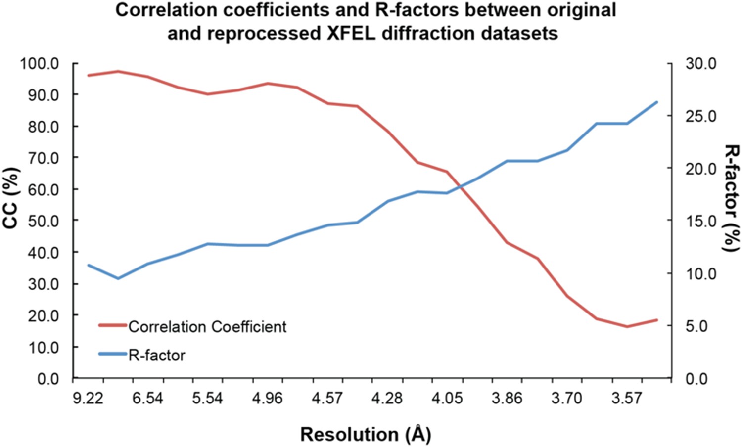
Statistical analysis of XFEL diffraction dataset reprocessing.
Correlation coefficients (red line) and R-values (blue line) between original and reprocessed XFEL diffraction datasets.
Author response image 2
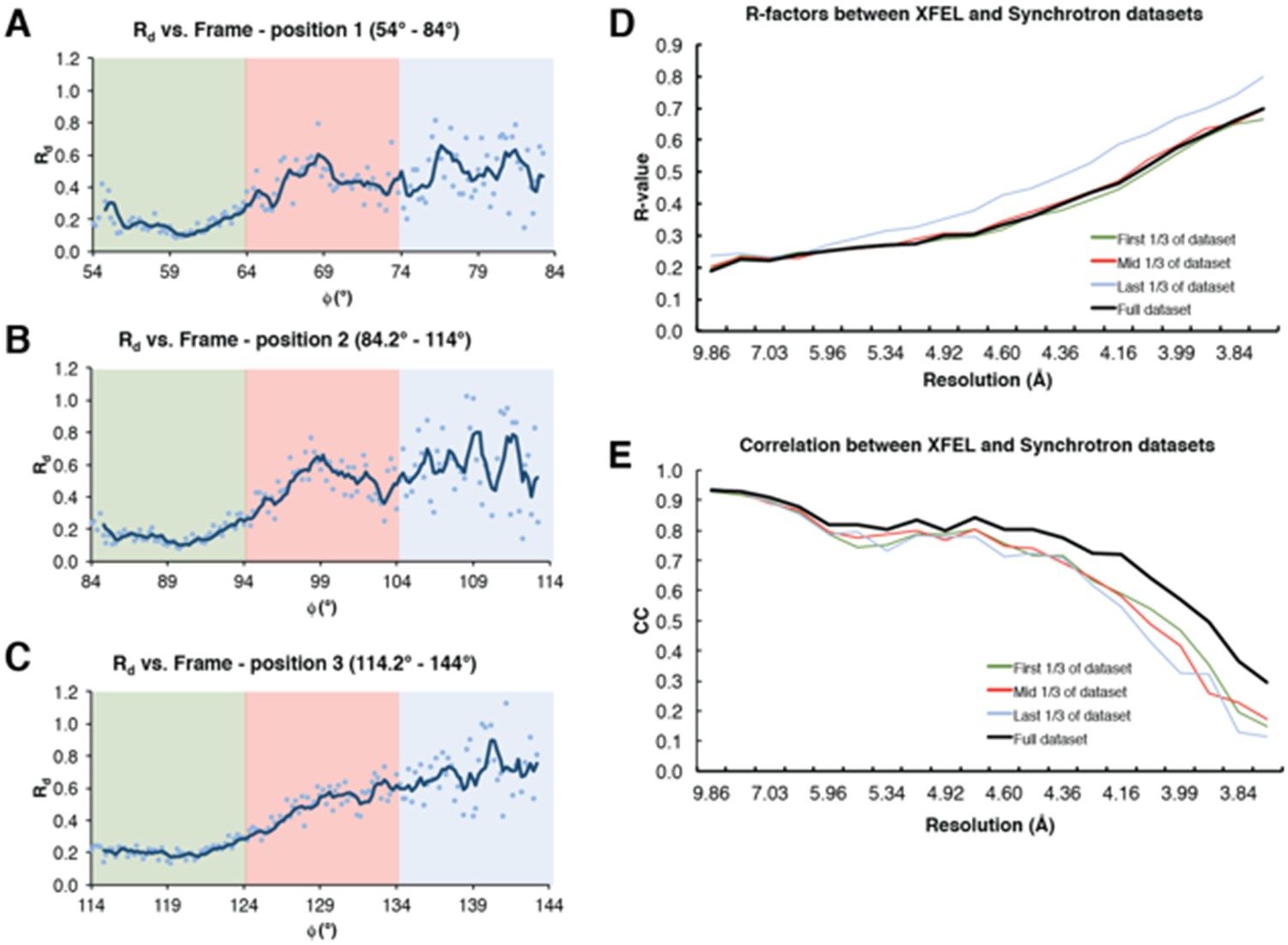
Analysis of radiation damage effect on synchrotron diffraction data.
(A–C) Rd plot vs. Φ angle for diffraction data collected at three separate positions on the same Syt1-SNARE crystal. Colored boxes represent sub-datasets (green – first 1/3 of the dataset, red – mid 1/3 of the dataset, blue – last 1/3 of the dataset). (D) R-factors between the full XFEL diffraction dataset and the three synchrotron sub-datasets; (E) Correlation coefficients between the two datasets. The colors for (D) and (E) follow the same scheme as that of (A–C); the full synchrotron dataset is shown as a black line.
Tables
Table 1
Data processing and refinement statistics for the synchrotron, XFEL, and simulated XFEL diffraction data.
| A. XFEL (SLAC-LCLS) | B. Synchroton (APS-NECAT) | C. Simulated XFEL (nanoBragg) | D. XFEL - Exclusion of negative intensities | E. XFEL - Exclusion of high resolution reflections | F. XFEL - Exclusion of low resolution reflections | G. Simulated XFEL – Exclusion of negative intensities | |
|---|---|---|---|---|---|---|---|
| No. images | 313 | 450 | 432 | 297 | 316 | 304 | 432 |
| Space group | P212121 | P212121 | P212121 | P212121 | P212121 | P212121 | P212121 |
| Cell dimensions* a, b, c (Å) | 69.5, 171.0, 291.3 | 68.8, 169.7, 286.8 | 69.4, 170.4, 291.0 | 69.4, 170.4, 291.0 | 69.5, 171, 291.4 | 69.6, 171, 291.4 | 69.4, 170.4, 291.0 |
| Resolution† (Å) | 20.0–3.5 (3.56–3.50) | 50.0–4.1 (4.21–4.10) | 20.0–3.5 (3.56–3.50) | 20.0–3.5 (3.56–3.50) | 20.0 – 4.1 (4.17–4.10) | 10.0 – 3.5 (3.56–3.50) | 20.0–3.5 (3.56–3.50) |
| Data cutoff [I / σ(I)] | −3 | −3 | −3 | .5 | −3 | −3 | .5 |
| Completeness (%) | 97.8 (89.2) | 98.1 (99.1) | 99.8 (99.1) | 87.8 (58.4) | 95.8 (84.2) | 88.3 (58.0) | 99.1 (95.5) |
| Multiplicity (rotation) ‡ | -- | 3.3 (3.4) | -- | -- | -- | -- | -- |
| Multiplicity (still) ‡ | 6.1 (2.9) | -- | 9.5 (6.7) | 4.4 (1.67) | 5.8 (3.1) | 4.3 (1.7) | 8.4 (4.8) |
| Post-refinement parameters | |||||||
| Linear scale factor G0 | 2.8 | -- | 1.9 | 2.9 | 3.9 | 2 | 1.3 |
| B | 66.8 | -- | 39.3 | 73.1 | 71.3 | 59.9 | 30.1 |
| γ0 (Å−1) | 0.00024 | -- | 0.00027 | 0.00016 | 0.00015 | 0.0014 | 0.00032 |
| γe (Å−1) | 0.00627 | -- | 0.00270 | 0.00483 | 0.00498 | 0.0639 | 0.00225 |
| Average Tpr | 169.8 | -- | 90.7 | 157.22 | 119.8 | 125.6 | 74.8 |
| Average Txy (mm2) | 7.3 | -- | 1.5 | 13.74 | 4.1 | 5.8 | 1.35 |
| CC1/2 | 94.3 (34.2) | 99.9 (63.8) | 99.1 (82.0) | 93.6 (43.4) | 94.3 (71.0) | 94.9 (41.7) | 99.4 (80.2) |
| Rmerge(%) (rotation) † | -- | 12.1 (78.8) | -- | -- | -- | -- | -- |
| Rmerge(%) (still) † | 49.4 (79.5) | -- | 17.3 (53.0) | 36.8 (33.5) | 38.3 (37.1) | 37.1 (32.8) | 13.0 (31.5) |
| I / σ(I) | 3.6 (0.2) | 7.6 (1.8) | 8.1 (1.6) | 4.7 (1.3) | 6.2 (1.8) | 3.5 (1.3) | 8.4 (2.4) |
| Structure-refinement parameters | |||||||
| Rwork / Rfree (%) | 29.2/32.9 | 28.8/ 29.5 | 9.6/11.1 | 30.0/33.2 | 28.9/33.5 | 31.5/34.6 | 10.7/12.5 |
| R.m.s. deviations | |||||||
| Bond lengths (Å) | 0.002 | 0.004 | 0.002 | 0.002 | 0.003 | 0.002 | 0.003 |
| Bond angles (° ) | 0.5 | 0.7 | 0.4 | 0.5 | 0.6 | 0.5 | 0.5 |
| No. atoms | |||||||
| Protein | 10578 | 10889 | 10578 | 10578 | 10903 | 10578 | 10578 |
| Ca2+ | 21 | 15 | 21 | 21 | 21 | 15 | 21 |
| B-factors | |||||||
| Protein | 106 | 155 | 40 | 52 | 103 | 64 | 43 |
| Ca2+ | 88 | 149 | 27 | 33 | 77 | 43 | 28 |
-
*The unit cell parameters displayed for XFEL data sets are the mean values of these parameters after post-refinement.
-
† Values in parentheses are for the highest resolution shell.
-
‡ '(rotation)' refers to rotation diffraction data collected at the synchrotron and '(still)'refers to XFEL diffraction data.
Table 2
Diffraction parameters for generation of the simulated XFEL diffraction data.
| Parameters | Values |
|---|---|
| Beam size (μm) | 30 |
| Spectral dispersion (Δλ/λ,%) | 0.2 |
| Wavelength jitter (%) | 0.5 |
| Intensity jitter* (%) | 100 |
| Beam center X, Y (mm) | 160.53, 182.31 |
| Misset angles (°) | 96.95, −52.09, −32.52 |
| Detector distance (mm) | 299.82 |
| Wavelength (Å) | 1.304735 |
| Mosaicity (°) | 0.2 |
| Divergence (mrad) | 0.02 |
| Dispersion (%) | 0.5 |
| Unit cell dimensions (a, b, c) (Å) | 69.6 171.1 291.9 |
| Mosaic domain size (μm) | 0.96 × 1.0 × 1.1 |
-
* Intensities were modeled using a Gaussian distribution with mean of 2 × 10¹² photons/pulse and FWHM of 2 × 10¹² photons/pulse.
Download links
A two-part list of links to download the article, or parts of the article, in various formats.
Downloads (link to download the article as PDF)
Open citations (links to open the citations from this article in various online reference manager services)
Cite this article (links to download the citations from this article in formats compatible with various reference manager tools)
Advances in X-ray free electron laser (XFEL) diffraction data processing applied to the crystal structure of the synaptotagmin-1 / SNARE complex
eLife 5:e18740.
https://doi.org/10.7554/eLife.18740


