Research Advance

Structural Biology and Molecular Biophysics

Advances in X-ray free electron laser (XFEL) diffraction data processing applied to the crystal structure of the synaptotagmin-1 / SNARE complex

Stanford University, United States
Lawrence Berkeley National Laboratory, United States
SLAC National Accelerator Laboratory, United States
University of California, San Francisco, United States

Oct 12, 2016

https://doi.org/10.7554/eLife.18740

Version of Record

Accepted for publication after peer review and revision.

Download
Cite
Share
CommentOpen annotations (there are currently 0 annotations on this page).

Version of Record published: November 3, 2016 (This version)
Accepted Manuscript published: October 12, 2016 (Go to version)
Accepted: October 11, 2016
Received: June 12, 2016

1. Builds upon
Enabling X-ray free electron laser crystallography for challenging biological systems from a limited number of crystals

Monarin Uervirojnangkoorn, Oliver B Zeldin ... William I Weis

Research Article Updated Apr 15, 2015
Further reading

Article
Figures and data
Abstract
Introduction
Results and discussion
Materials and methods
Data availability
References
Decision letter
Author response
Article and author information
Metrics

Abstract

X-ray free electron lasers (XFELs) reduce the effects of radiation damage on macromolecular diffraction data and thereby extend the limiting resolution. Previously, we adapted classical post-refinement techniques to XFEL diffraction data to produce accurate diffraction data sets from a limited number of diffraction images (Uervirojnangkoorn et al., 2015), and went on to use these techniques to obtain a complete data set from crystals of the synaptotagmin-1 / SNARE complex and to determine the structure at 3.5 Å resolution (Zhou et al., 2015). Here, we describe new advances in our methods and present a reprocessed XFEL data set of the synaptotagmin-1 / SNARE complex. The reprocessing produced small improvements in electron density maps and the refined atomic model. The maps also contained more information than those of a lower resolution (4.1 Å) synchrotron data set. Processing a set of simulated XFEL diffraction images revealed that our methods yield accurate data and atomic models.

https://doi.org/10.7554/eLife.18740.001

Introduction

X-ray free electron laser (XFEL) crystallography is an emerging technique for obtaining high-resolution diffraction data from macromolecular crystals (Schlichting, 2015). Diffraction data from an XFEL pulse lasting only tens of femtoseconds are largely free from X-ray induced radiation damage that might otherwise affect the success of crystallographic phasing and atomic model refinement. However, the crystal is effectively stationary during the XFEL pulse, which complicates determination of the crystal lattice model from the resulting zero-rotation or 'still' diffraction images. Furthermore, the XFEL pulse destroys or damages the illuminated crystal volume and thus allows only a single diffraction image to be collected. This effect is exacerbated by the variation in intensity and spectrum of the incident XFEL beam produced by the self-amplified spontaneous emission (SASE) process (Bonifacio et al., 1994; Emma et al., 2010). Together, these features cause significant image-to-image variability in the diffraction data (Hattne et al., 2014; Kern et al., 2012; Lyubimov et al., 2016; Sauter, 2015) and therefore pose challenges for data processing. Early XFEL diffraction data sets were processed exclusively using 'Monte Carlo' summation methods (Kirian et al., 2010), which required large numbers of diffraction images.

Previously, we described a program, PRIME, that uses post-refinement techniques to improve the scaling and merging of XFEL data sets obtained from relatively small numbers (100–2000) of diffraction patterns (Uervirojnangkoorn et al., 2015). This method, and similar methods described by others (Kabsch, 2014; Kroon-Batenburg et al., 2015; White, 2014; Ginn et al., 2015a) were applied to diffraction data of crystals of known structure (White, 2014; Kabsch, 2014; Lyubimov et al., 2015; Murray et al., 2015; Ginn et al., 2015b). We subsequently successfully applied our methods to the previously unknown crystal structure of the complex between synaptotagmin-1 (Syt1) and the neuronal SNARE complex, which mediates the fusion of synaptic vesicles with the synaptic membrane and is essential for Ca²⁺-dependent neurotransmitter release (Zhou et al., 2015). We had only a limited number of relatively large, plate-like crystals available that were not suitable for liquid jet experiments, so the XFEL diffraction data were collected on the goniometer setup implemented at the X-ray Pump Probe (XPP) endstation of the Linac Coherent Lightsource (LCLS) at SLAC National Accelerator Laboratory (Cohen et al., 2014).

To date, several structures have been determined using relatively small numbers of diffraction images obtained from crystals of known structure that diffracted to high resolutions (Cohen et al., 2014; Lyubimov et al., 2015; Uervirojnangkoorn et al., 2015; Hirata et al., 2014; Suga et al., 2015). Although valuable as test cases for methods development, they were not challenging enough to test the limits of XFEL data processing methods. In contrast, the Syt1–SNARE XFEL diffraction data set contained two crystal forms indistinguishable by visual inspection and had a limiting resolution of ~3.5 Å. These diffraction data required us to improve our data processing methods.

Here we describe improvements to PRIME (Uervirojnangkoorn et al., 2015) and other parts of the data processing system. We reprocessed the XFEL diffraction data of the Syt1–SNARE complex, which resulted in small improvements to the data and the atomic model refined against these data. We verified the accuracy of these improved methods by processing a simulated a XFEL diffraction data set that mimicked the Syt1–SNARE XFEL experiment. We also compared the reprocessed XFEL diffraction data set to a synchrotron diffraction data set collected from a similar Syt1–SNARE crystal. The synchrotron data extended to lower resolution (4.1 Å) and consequently provided less detailed electron density maps. Nonetheless, comparison with XFEL-derived maps calculated to 4.1 Å resolution showed that the XFEL maps were slightly more interpretable. We conclude that our methods have general applicability to XFEL diffraction data processing.

Results and discussion

Reprocessing the 3.5 Å XFEL diffraction data of the Syt1–SNARE complex

As previously described (Zhou et al., 2015), we used the program cctbx.xfel (Hattne et al., 2014) to index and integrate the observed XFEL diffraction images of crystals of the Syt1-SNARE complex. We performed a grid search of spot-finding parameters on an image-to-image basis to maximize the success of indexing and integration (Lyubimov et al., 2016). We divided the diffraction images into individual clusters based on their crystal symmetry and unit cell parameters using hierarchical clustering (Andrews and Bernstein, 2014; Zeldin et al., 2015). Using the largest cluster, we employed post-refinement as implemented in the program PRIME (Uervirojnangkoorn et al., 2015) to generate a merged diffraction data set from the relatively limited number of diffraction images. Two previously unpublished features were necessary to obtain the best results possible at the time, and are described in detail in the methods. First, the crystal lattice model refinement algorithm in cctbx.xfel was enhanced in order to minimize instances of mis-indexing. Second, an improved scaling procedure was implemented in PRIME.

Subsequent to the original publication (Zhou et al., 2015), we further enhanced the data processing methods. We combined the IOTA grid search method (Lyubimov et al., 2016) with new features including automatic rejection of images that had no discernible diffraction, the ability to use information about the Bravais lattice and unit cell dimensions from other data, and detection of mis-indexed images. We also implemented a graphical user interface for the processing of XFEL diffraction images. As described in the Materials and methods, the cctbx.xfel algorithms were also modified to allow refinement of parameters such as detector position and tilt. Finally, we introduced a feature to include reflections with negative intensity measurements in merging and post-refinement with PRIME.

We reprocessed the XFEL diffraction data of the Syt1–SNARE complex at 3.5 Å resolution to take advantage of all improvements implemented since the original publication (Zhou et al., 2015). Of the 789 diffraction images collected from 148 crystals, 362 images were indexed in the 'long unit cell' crystal form (see Materials and methods); this was the largest of the unit cell 'clusters' determined by the Andrews-Bernstein algorithm (Andrews and Bernstein, 2014 ; Zeldin et al., 2015). Of these, 328 images could be successfully integrated. Of the 328 integrated images, 15 were rejected during post-refinement, and the remaining 313 were merged into the final scaled data set (Table 1A).

Table 1

Data processing and refinement statistics for the synchrotron, XFEL, and simulated XFEL diffraction data.

https://doi.org/10.7554/eLife.18740.002

	A. XFEL (SLAC-LCLS)	B. Synchroton (APS-NECAT)	C. Simulated XFEL (nanoBragg)	D. XFEL - Exclusion of negative intensities	E. XFEL - Exclusion of high resolution reflections	F. XFEL - Exclusion of low resolution reflections	G. Simulated XFEL – Exclusion of negative intensities
No. images	313	450	432	297	316	304	432
Space group	P2₁2₁2₁	P2₁2₁2₁	P2₁2₁2₁	P2₁2₁2₁	P2₁2₁2₁	P2₁2₁2₁	P2₁2₁2₁
Cell dimensions* a, b, c (Å)	69.5, 171.0, 291.3	68.8, 169.7, 286.8	69.4, 170.4, 291.0	69.4, 170.4, 291.0	69.5, 171, 291.4	69.6, 171, 291.4	69.4, 170.4, 291.0
Resolution^† (Å)	20.0–3.5 (3.56–3.50)	50.0–4.1 (4.21–4.10)	20.0–3.5 (3.56–3.50)	20.0–3.5 (3.56–3.50)	20.0 – 4.1 (4.17–4.10)	10.0 – 3.5 (3.56–3.50)	20.0–3.5 (3.56–3.50)
Data cutoff [I / σ(I)]	−3	−3	−3	.5	−3	−3	.5
Completeness (%)	97.8 (89.2)	98.1 (99.1)	99.8 (99.1)	87.8 (58.4)	95.8 (84.2)	88.3 (58.0)	99.1 (95.5)
Multiplicity (rotation) ^‡	--	3.3 (3.4)	--	--	--	--	--
Multiplicity (still) ^‡	6.1 (2.9)	--	9.5 (6.7)	4.4 (1.67)	5.8 (3.1)	4.3 (1.7)	8.4 (4.8)
Post-refinement parameters
Linear scale factor G₀	2.8	--	1.9	2.9	3.9	2	1.3
B	66.8	--	39.3	73.1	71.3	59.9	30.1
γ₀ (Å⁻¹)	0.00024	--	0.00027	0.00016	0.00015	0.0014	0.00032
γ_e (Å⁻¹)	0.00627	--	0.00270	0.00483	0.00498	0.0639	0.00225
Average T_pr	169.8	--	90.7	157.22	119.8	125.6	74.8
Average T_xy (mm²)	7.3	--	1.5	13.74	4.1	5.8	1.35
CC_1/2	94.3 (34.2)	99.9 (63.8)	99.1 (82.0)	93.6 (43.4)	94.3 (71.0)	94.9 (41.7)	99.4 (80.2)
R_merge(%) (rotation) ^†	--	12.1 (78.8)	--	--	--	--	--
R_merge(%) (still) ^†	49.4 (79.5)	--	17.3 (53.0)	36.8 (33.5)	38.3 (37.1)	37.1 (32.8)	13.0 (31.5)
I / σ(I)	3.6 (0.2)	7.6 (1.8)	8.1 (1.6)	4.7 (1.3)	6.2 (1.8)	3.5 (1.3)	8.4 (2.4)
Structure-refinement parameters
R_work / R_free (%)	29.2/32.9	28.8/ 29.5	9.6/11.1	30.0/33.2	28.9/33.5	31.5/34.6	10.7/12.5
R.m.s. deviations
Bond lengths (Å)	0.002	0.004	0.002	0.002	0.003	0.002	0.003
Bond angles (° )	0.5	0.7	0.4	0.5	0.6	0.5	0.5
No. atoms
Protein	10578	10889	10578	10578	10903	10578	10578
Ca²⁺	21	15	21	21	21	15	21
B-factors
Protein	106	155	40	52	103	64	43
Ca²⁺	88	149	27	33	77	43	28

*The unit cell parameters displayed for XFEL data sets are the mean values of these parameters after post-refinement.
† Values in parentheses are for the highest resolution shell.
‡ '(rotation)' refers to rotation diffraction data collected at the synchrotron and '(still)'refers to XFEL diffraction data.

As in the originally published Syt1–SNARE structure, we observed strong electron density for many side chains (Figure 1A,B). Our modified data processing methods resulted in small improvements in the refinement statistics of the Syt1–SNARE structure (Table 1A) vs. the originally published structure (Zhou et al., 2015). Moreover, the reprocessed XFEL diffraction data produced slightly more interpretable electron density maps, which in a few cases allowed better modeling of side chain rotamers that were previously difficult to interpret (Figure 1—figure supplement 1). Simulated annealing composite omit maps (Figure 1—figure supplement 2) indicated that the electron densities observed in the XFEL-data derived maps are not likely affected by potential model bias.

Figure 1 with 2 supplements see all

Download asset Open asset

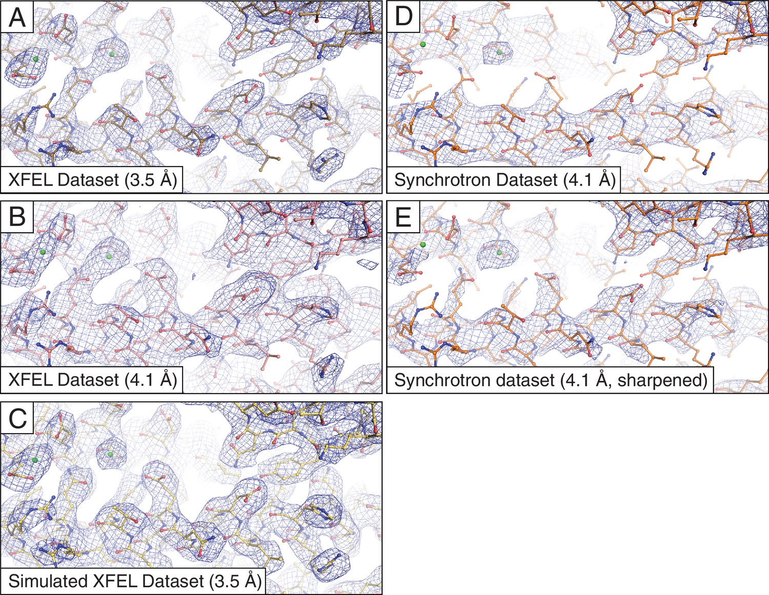
Representative *2mF_o-DF_c* electron density maps.

The maps were obtained using (A) the XFEL diffraction data at 3.5 Å resolution; (B) same as (A) but truncated to 4.1 Å resolution in order to match the limiting resolution of the synchrotron data; (C) the simulated XFEL diffraction data set; (D) the synchrotron data set (at 4.1 Å resolution), (E) same as (D) but with the synchrotron data sharpened with B_sharp = −23 Å² in order to account for the differences in overall B-factors of the corresponding diffraction data sets. All maps were rendered at a contour level of 2.0 σ.

https://doi.org/10.7554/eLife.18740.003

As a further assessment of the Syt1–SNARE XFEL diffraction data reprocessing, we re-refined the most current atomic model against the original XFEL diffraction data, resulting in R_work = 31.1% and R_free = 33.6%. Since the original XFEL diffraction data did not include negative intensity measurements, we also re-refined the current model against the reprocessed data set including only reflections with positive measurements. R_work and R_free were 1.1% and 0.4% lower, respectively, than those for the original XFEL diffraction data (Table 1D), indicating that the reprocessed data are more accurate than the original data. Inclusion of negative intensity measurements further lowered R_work and R_free by 0.8% and 0.3%, respectively, for the reprocessed data (Table 1A), indicating that the inclusion of negative intensities results in a somewhat more accurate model, which could be due to improved data completeness, accuracy, or both.

Accuracy of data processing with simulated XFEL diffraction images

In order to assess if our improved data processing system could accurately process XFEL still data, we generated a simulated XFEL diffraction data set from the atomic coordinates of the Syt1–SNARE complex (Materials and methods) and processed it with the same methods used for the observed XFEL data. This produced a merged dataset with excellent CC_1/2, R_merge and I / σ(I) values (Table 1C) and good agreement with structure factors calculated from the Syt1–SNARE structure that were used to generate the simulated XFEL data set [CC = 97.5% (88.4% in the high resolution bin), R = 11.8% (35.1% in the high resolution bin)]. The atomic model of the Syt1–SNARE complex was then re-refined against the simulated XFEL dataset, resulting in low R-values (Table 1C) and good agreement with the structure that was used to generate the simulated data set (root-mean-square-difference = 0.11 Å). Moreover, electron density maps computed from the simulated XFEL dataset showed strong features for most side chains (Figure 1C). Thus, our data processing system can produce a reasonably accurate merged diffraction data set from simulated XFEL still images. However, the CC_1/2 of the observed XFEL diffraction data and the R values of the corresponding refined atomic model are inferior to those obtained from the simulated XFEL data set (Table 1A). Although this difference might arise from experimental noise, it may also indicate that the simulation does not fully account for certain features of the observed XFEL data.

Comparison to 4.1 Å synchrotron diffraction data of the Syt1-SNARE complex

We previously reported diffraction data sets from crystals of the Syt1-SNARE complex collected at a microfocus synchrotron beam line using rotation data collection (Zhou et al., 2015). These synchrotron data sets, however, were obtained from a different (short unit cell') crystal form than that for the XFEL-data derived Syt1–SNARE crystal structure (Zhou et al., 2015). Here we have measured a synchrotron data set from a similar crystal in the same long unit cell' crystal form used for the XFEL-data derived structure (Table 1B).

A key difference between the XFEL and synchrotron data is the higher limiting resolution of the XFEL diffraction data (3.5 Å vs. 4.1 Å, Table 1A, B). The synchrotron diffraction data were obtained from a single crystal judged to be the best from a pool screened for optimal diffraction, and 4.1 Å was determined to be the maximum achievable limiting resolution with this particular data set. In contrast, the XFEL diffraction data were obtained from 148 crystals of widely varying quality with limiting resolutions ranging from ~5 Å to 2.9 Å (in 92 cases). Even though only 313 XFEL diffraction images were used in the final merged data set, it had high completeness (97.8%) and good multiplicity (6.1), along with reasonable merging statistics to 3.5 Å resolution (Table 1A). Notably, more diffraction images (450) were used in the synchrotron data set.

For more precise comparison, we re-scaled the synchrotron data to the same isotropic temperature factor (B) value as that of the XFEL data by applying a (sharpening) B factor of −23 Å². Subsequent re-refinement of the atomic model produced only a slight improvement in the electron density map (Figures 1D,E). We also tested the effect of the different resolution limits of the XFEL and synchrotron data sets by reprocessing the XFEL data truncated to 4.1 Å resolution, followed by atomic model refinement (Table 1E). Although the synchrotron data-derived model refined to a lower R_free value than the XFEL data-derived model (29.5% vs. 32.9%), the electron density maps calculated from the XFEL data set (Figures 1A,B) generally contained more information than the synchrotron data-derived maps (Figure 1D), even when the latter were sharpened (Figure 1E). The same effect was found using simulated annealing composite omit maps (Figure 1—figure supplement 2), suggesting that the side chain density features of the XFEL data-derived maps are not the result of model bias.

The electron density maps were quantitatively assessed by the real-space correlation coefficient (CC) calculated for each amino acid type (Figure 2). The real-space CCs were calculated using phenix.get_cc_mtz_pdb (Adams et al., 2010) by comparing a likelihood-weighted 2mF_o-DF_c electron density map with a map calculated from the model. All amino acid types correlate better with the XFEL data-derived map than with the corresponding synchrotron data-derived map (Figure 2A). Additionally, more Ca²⁺ were visible in the XFEL-data derived maps (21 Ca²⁺) than in synchrotron-data derived maps (15 Ca²⁺). The 13 Ca²⁺ that were in matching positions in both maps had higher real-space CCs in the XFEL-data derived structure (Figure 2C). Similar, but somewhat less pronounced results were obtained when calculating the real-space correlation coefficients from the simulated annealing composite omit maps (Figure 2—figure supplement 1).

Figure 2 with 1 supplement see all

Download asset Open asset

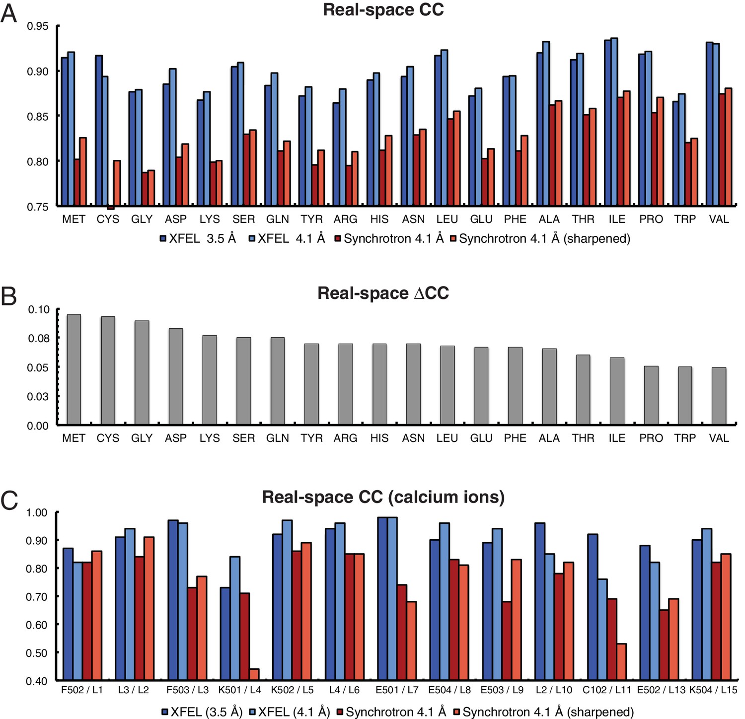
Analysis of real-space correlation for atomic models refined against the XFEL and synchrotron data sets.

(A) Real-space correlation coefficients for atomic models of the Syt1–SNARE complex refined against the XFEL (XFEL 3.5 Å, XFEL 4.1 Å) and synchrotron [Synchrotron 4.1 Å, Synchrotron 4.1 Å (sharpened)] diffraction data and analyzed by amino acid residue type; (B) differences between real-space correlation coefficients of the atomic models (ΔCC) refined against the XFEL and synchrotron diffraction data of Syt1–SNARE complex, both processed and refined at 4.1 Å resolution; (C) real-space correlation coefficients for the Ca²⁺ sites that were visible in the XFEL- and synchrotron-data derived Syt1–SNARE crystal structures (due to the different numbering of calcium ions in XFEL- and synchrotron-derived structures, two chain and atom labels are given for each, e.g. “F502 / L1”; the first label refers to the XFEL-derived structure, while the second label refers to the synchrotron-derived structure). To facilitate the comparison, the XFEL-based correlation coefficients were calculated at a limiting resolution of 4.1 Å (matching the limiting resolution of the synchrotron data set) as well as at the actual limiting resolution of the XFEL diffraction data set (3.5 Å). Furthermore, the electron density maps obtained from the synchrotron data were sharpened with B_sharp = −23 Å² in order to account for the difference in overall B-factors of the diffraction data sets.

https://doi.org/10.7554/eLife.18740.006

Although the differences between XFEL and synchrotron data sets may be due to differences in radiation damage sustained by the crystals during X-ray exposure, they may have arisen from batch-to-batch differences in crystal quality, individual crystal-to-crystal variability, differences in data collection strategy, or a combination of all these factors. Further studies will be required to determine whether XFELs can improve upon the diffraction data obtained from synchrotrons.

Conclusions

Advances to our XFEL diffraction data processing system resulted in somewhat better statistics of a diffraction data set and refined atomic model for the crystal structure of the Syt1–SNARE complex than that previously reported (Zhou et al., 2015). Compared with a lower resolution synchrotron diffraction data set obtained from similar crystals in the same crystal form, the electron density maps calculated from the XFEL data contained more information, especially for many side chains. However, the statistics of the XFEL diffraction data (CC_1/2) and refined atomic model (R_work and R_free) are still inferior to those obtained from synchrotron data (Table 1). The accuracy of a merged data set obtained from simulated XFEL diffraction images (Table 1) and the accuracy of an atomic model that was refined against it indicate that the differences in refinement statistics cannot be explained by an inability to adequately recover partiality and scaling information from a 'perfect' XFEL diffraction data set. We expect that further improvements in modeling the properties of XFEL diffraction data (Hattne et al., 2014; Lyubimov et al., 2016; Sauter, 2015), such as pulse-to-pulse variation in the SASE spectrum (Emma et al., 2010; Bonifacio et al., 1994), along with different modes of XFEL beam generation (Amann et al., 2012), should further improve the statistics of the XFEL diffraction data and ultimately approach those of synchrotron crystallography.

Materials and methods

Crystallization of the Syt1–SNARE complex

Request a detailed protocol

Construct design, cloning, expression, purification and crystallization of the Syt1–SNARE complex have been previously described (Zhou et al., 2015), and are briefly summarized here. Crystallization took 1–3 months, making the optimization of the crystals a difficult and time-consuming process. All crystals appeared as single plates approximately 25 × 250 × 500 μm³ and were mounted using 0.4–0.7 mm cryo-loops. Due to surface tension, the mounted crystals rested in the same plane as the cryo-loops. The mounted crystals were flash-cooled in a cryo-protecting solution containing the same constituents as the crystallization condition (20 mM Tris-HCl pH 8.0, 300 mM NaCl, 100 mM MgCl₂, 1 mM CaCl₂, and 0.5 mM TCEP in the protein buffer and 100 mM HEPES-Na pH 7.5 and 1% PEG 8000 in the reservoir buffer) supplemented with 35% (v/v) sucrose. The Syt1–SNARE complex crystallizes in two distinct crystal forms with morphologies that were indistinguishable by inspection of the crystals. As one of these crystal forms arose by the doubling of a single axis of the other crystal form, we term these 'long unit cell' and 'short unit cell' crystal forms, respectively (Zhou et al., 2015; Zeldin et al., 2015; Lyubimov et al., 2016).

XFEL data collection

Request a detailed protocol

Collection of the Syt1–SNARE XFEL diffraction data has been described (Zhou et al., 2015) and is briefly summarized here. The XFEL data were collected at the X-ray Pump Probe (XPP) endstation of the Linac Coherent Light Source (LCLS) at the SLAC National Accelerator Laboratory, using a goniometer-based fixed target sample delivery station and an automatic sample loading system similar to the setup used for conventional synchrotron data collection at SSRL (Cohen et al., 2002, 2014). We used a 30 μm XFEL beam with a pulse duration of 40 fs in SASE mode. We calculated the centroid of the SASE energy spectrum and used this value for the wavelength input to post-refinement of each diffraction image. Each 40 fs XFEL pulse at the XPP endstation at LCLS delivers approximately 10¹² photons, depositing a dose of 0.5 MGy. A total of 148 crystals were screened, yielding 789 images with usable diffraction.

Simulated XFEL data

Request a detailed protocol

To better understand some of the persistent problems found when integrating the intensities of XFEL data, we simulated XFEL diffraction images (Table 2, Figure 3) from the previously deposited structure of the Syt1–SNARE complex (PDB ID 5CCG). We calculated structure factors from these coordinates to 3.0 Å resolution with bulk solvent model parameters k_sol = 0.3 e/Å³ and B_sol = 50 Å² using CNS (Brunger et al., 1998). XFEL still diffraction images were simulated using the program nanoBragg (http://bl831.als.lbl.gov/~jamesh/nanoBragg/) with parameters shown in Table 2. These parameters were optimized using a brute-force grid search scored by the Pearson correlation coefficient between the simulated image and a single observed XFEL diffraction image with a high number of strong, well-resolved Bragg peaks, hand-selected from the Syt1–SNARE complex XFEL data set. To expedite the comparisons, pixels far from observed spots were excluded using a mask derived from blurring the background-subtracted real image. The point-spread function of the fiber-coupled CCD detector was implemented as described previously (Holton et al., 2012), and the conventional mosaic spread (Helliwell et al., 1982) was represented by 675 discrete mosaic domains distributed isotropically and randomly over a spherical cap with diameter 0.2 deg. Beam divergence and dispersion were simulated using four discrete source points, separated by the desired divergence, each emitting six discrete wavelengths evenly spaced across the desired spectral width (Table 2). The experimentally observed X-ray background was extracted with the fastBragg companion program nonBragg using a median-filtered azimuthal average for constant-resolution rings of pixels. This radial profile was subsequently used to simulate the X-ray background level. Finally, a hand-drawn beam stop shadow was applied to the simulated images. Apart from the random number seed used to generate noise, the final 432 simulated XFEL diffraction images varied from each other only in crystal orientation and the beam intensity, which were randomized shot-to-shot.

Table 2

Diffraction parameters for generation of the simulated XFEL diffraction data.

https://doi.org/10.7554/eLife.18740.008

Parameters	Values
Beam size (μm)	30
Spectral dispersion (Δλ/λ,%)	0.2
Wavelength jitter (%)	0.5
Intensity jitter* (%)	100
Beam center X, Y (mm)	160.53, 182.31
Misset angles (°)	96.95, −52.09, −32.52
Detector distance (mm)	299.82
Wavelength (Å)	1.304735
Mosaicity (°)	0.2
Divergence (mrad)	0.02
Dispersion (%)	0.5
Unit cell dimensions (a, b, c) (Å)	69.6 171.1 291.9
Mosaic domain size (μm)	0.96 × 1.0 × 1.1

* Intensities were modeled using a Gaussian distribution with mean of 2 × 10¹² photons/pulse and FWHM of 2 × 10¹² photons/pulse.

Figure 3

Download asset Open asset

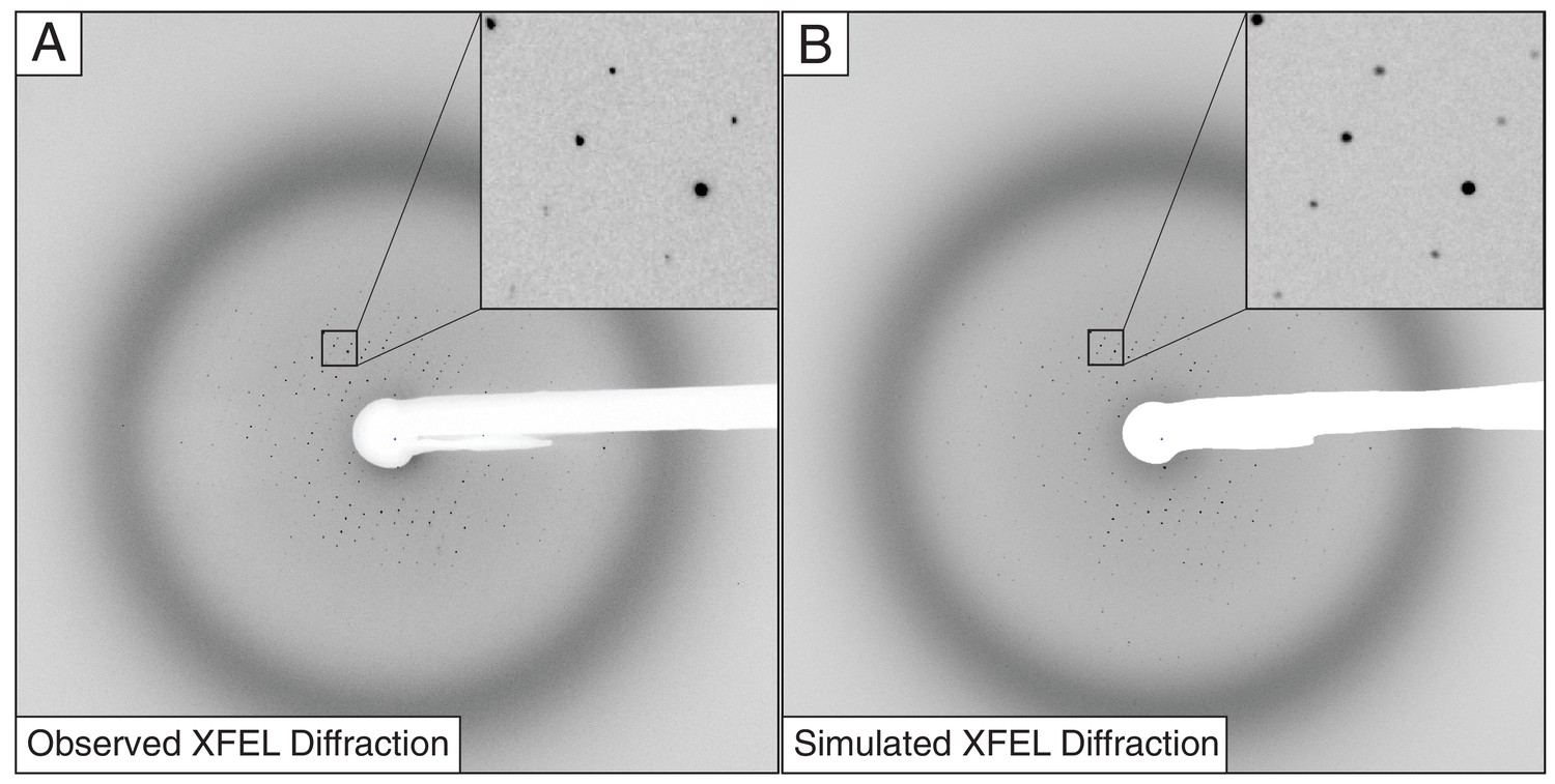
Observed (A) and simulated (B) XFEL diffraction images of the Syt1–SNARE complex.

The insets show close-up views of the indicated regions.

https://doi.org/10.7554/eLife.18740.009

XFEL diffraction data reprocessing

Request a detailed protocol

The experimental and the simulated XFEL diffraction images were indexed and integrated using identical procedures (Figure 4). We used cctbx.xfel (Hattne et al., 2014) with the improvements outlined below, along with the latest version of IOTA (Lyubimov et al., 2016), which enabled proper processing of a few additional diffraction images that had been previously mis-indexed. A hierarchical clustering algorithm (Andrews and Bernstein, 2014; Zeldin et al., 2015) was used to separate the two crystal forms found in the experimental XFEL diffraction images. Integrated diffraction images were scaled, merged and post-refined using PRIME (Uervirojnangkoorn et al., 2015) with improvements in scaling as outlined below.

Figure 4 with 4 supplements see all

Download asset Open asset

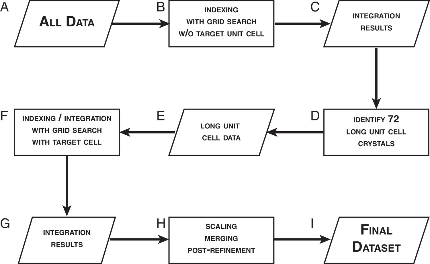
Data processing strategy for XFEL diffraction data of the Syt1–SNARE complex.
https://doi.org/10.7554/eLife.18740.010

Improvements to indexing, integration, and scaling

Request a detailed protocol

Several previously unpublished improvements to the core modules of the cctbx.xfel suite of software were required in order to successfully index and integrate diffraction images obtained from the Syt1–SNARE crystals using XFEL radiation:

We found that a small number of images of the Syt1–SNARE XFEL data set were mis-indexed. To alleviate this problem, we added the option to retain the initial assignment of Miller indices to Bragg reflections to cctbx.xfel (Young et al., 2016). During the indexing step, cctbx.xfel determines and refines the three basis vectors that span the primitive triclinic lattice, which are then used to assign Miller indices to the strong Bragg reflections found on the diffraction image. Subsequently, possible crystal symmetry constraints are applied to the lattice model. In the previous work (Zhou et al., 2015), Miller indices of the strong spots were then re-determined based on their proximity to nodes on the symmetry-constrained lattice. This was found to be problematic in cases where a long unit cell axis causes lattice nodes to be positioned close together, which may cause incorrect re-assignment of Miller indices. Mis-indexing was suppressed by retaining the original triclinic Miller index assignments throughout the re-refinement of the symmetry-constrained lattice model, while applying the appropriate change-of-basis operator to convert the indices to the appropriate symmetry (Sauter et al., 2006). Note that this approach does not correct any indexing errors that might have occurred during the initial indexing step.
Lattice model refinement is now carried out using modules from the DIALS toolkit (Waterman et al., 2016), wherein the target function includes both positions of the observed Bragg reflections and the angular proximity of reciprocal lattice points to the Ewald sphere as described previously (Sauter et al., 2014). DIALS allows the refinement of additional parameters such as detector tilt and distance, which substantially increases the success of obtaining a lattice model that best correlates with observed diffraction (Figure 4—figure supplement 1).
Partial reflections with negative intensities after background subtraction are now included in both cctbx.xfel and PRIME. Approximately 30% of the background subtracted integrated reflection intensities on XFEL diffraction images of the Syt1–SNARE crystals have negative values (Hattne et al., 2014; Sauter et al., 2014). We found that inclusion of these measurements alleviated unusual behavior of the L-test (Padilla and Yeates, 2003) and made the L-test of the XFEL data set comparable to that of the synchrotron data set (Figure 4—figure supplement 2). (Note that merohedral twinning is not possible in this crystal form.) While further investigations are underway to understand the impact of negative intensities and post-refinement on the statistics of the merged data set, we have added an option in PRIME to include negative intensity measurements in post-refinement. Currently, the default is to set the threshold at $I / σ (I) > - 3.0$ for reflections used in scale factor and diffraction parameter refinement, and this default was used for the final data set shown in Table 1A. The merging statistics for the observed XFEL diffraction data set with negative intensities excluded are shown in Table 1D.

Indexing and integration of the XFEL diffraction images

Request a detailed protocol

Typically, when processing XFEL diffraction data of a known system using cctbx.xfel, one would supply the known crystal symmetry and unit cell data as target parameters in order to better guide the lattice model refinement. However, this approach is not suitable for a system such as Syt1–SNARE complex, where a batch typically contains crystals in two related, but distinct orthorhombic unit cells (Zhou et al., 2015). In this case, using a single target unit cell to process diffraction data from two similar crystal forms would be inappropriate, as incorrect unit cell parameters could be forced upon images. Furthermore, since the Syt1–SNARE complex structure was unknown at the time, and the only information about the unit cell parameters was from lower-resolution synchrotron diffraction data, we were not confident that the available unit cell information would apply to the XFEL diffraction data set. To circumvent these difficulties, we utilized a multi-step data processing strategy (Figure 4).

We began by pooling all 789 XFEL diffraction images regardless of which crystal form they were from (Figure 4A), and indexed them without supplying any target unit cell parameters (Figure 4B). At this stage, we employed a spot-finding parameter grid search using the program IOTA (Lyubimov et al., 2016), which was specially developed for the purpose of optimizing the processing of XFEL diffraction stills. We used the unit cell information obtained from these indexed diffraction images (Figure 4C) and performed a hierarchical cluster analysis of these unit cells (Andrews and Bernstein, 2014; Zeldin et al., 2015). We then correlated each indexed image with the crystal it was obtained from, and identified 72 crystals that belonged to the 'long unit cell' (a = 69.4 Å, b = 170.8 Å, c = 291.2 Å, α = β = γ = 90°) crystal form (Figure 4D). The 362 diffraction images obtained from these 72 crystals comprised the 'long unit cell' cluster (Figure 4E). Only this crystal form yielded a sufficient number of diffraction images for a complete data set. The remaining 427 images that were either assigned to the 'short unit cell' cluster, could not be indexed, or contained no interpretable diffraction, were excluded from further analysis.

The clustering algorithm produced a set of consensus unit cell parameters that are assigned to the 'long unit cell' cluster. We used these unit cell parameters as a target for the indexing and integration of the 362 'long unit cell'diffraction images. At this stage, we performed an extensive spot-finding parameter grid search (minimum spot area = 2–22 pixels, minimum spot height = 2–15 σ, Figure 4F). Interestingly, this produced a wide range of spot-finding parameters that would yield optimal integration results (Figure 4—figure supplement 3A). An identical grid search carried out for the set of simulated XFEL diffraction images (described below) yielded a much narrower distribution (Figure 4—figure supplement 3B), illustrating the high degree of shot-to-shot variability inherent in XFEL diffraction data.

Of the 362 'long unit cell' diffraction images, 328 images were successfully integrated using the wide grid search parameters, while 34 images could not be integrated for a variety of reasons (insufficient number of Bragg reflections, poor diffraction quality, or un-resolvable multiple lattices). The 328 successfully integrated diffraction images were used as input for scaling, post-refinement and merging using the program PRIME. Of those 328 integrated diffraction images, 15 were rejected during post-processing due to large deviations from refined mean values for unit cell and scaling parameters. The remaining 313 integrated diffraction images were included in the final merged XFEL data set (Figure 4G–I, Table 1A).

Analysis of refined direct beam coordinates identifies mis-indexed XFEL images

Request a detailed protocol

Processing of the simulated XFEL diffraction data set with cctbx.xfel revealed occasional incidents of mis-indexing by a shift of a Miller index by ± 1. Since even a few mis-indexed frames can adversely affect the statistics of a merged diffraction data set, a diagnostic tool to detect them early would be desirable. We found that a plot of the refined direct beam coordinates can identify mis-indexed diffraction images in the experimental XFEL data set (Figure 4—figure supplement 4).

We have shown previously that probable position(s) for the direct beam position on the detector can be deduced from the periodic repeat of bright spots (Sauter et al., 2004), given an initial estimate of the beam position derived from the refined detector metrology (Hattne et al., 2014). Probability maps for the direct beam position have been useful for data collected at synchrotron beamlines, in cases where the beam position is not correctly recorded with the image metadata. Searching for probable beam positions up to a radius of 4 mm around the initial position allows the indexing program LABELIT to estimate the true position. However, we found it counterproductive to apply such a wide beam search to XFEL data. Firstly, at the XPP endstation the beam position with respect to the detector is known within ± 100 μm. Secondly, allowing a large search radius can potentially identify an incorrect beam position. In the case of the Syt1–SNARE complex XFEL diffraction data, eight mis-indexed frames exhibited a shift of ~1.5 mm in beam position, corresponding to a shift of one lattice spacing along the long c-axis (291 Å, Figure 4—figure supplement 4A). We therefore limited the beam search scope to a radius of 0.5 mm. Under this condition only two XFEL diffraction images remained mis-indexed (Figure 4—figure supplement 4B), and were therefore omitted from the merged diffraction data set.

Scaling, post-refinement, and merging of the XFEL data sets

Request a detailed protocol

Integrated XFEL images in the long unit cell cluster were scaled, post-refined and merged with PRIME, which corrects partially recorded intensities to their full intensity values using a partiality model (Uervirojnangkoorn et al., 2015). This step begins with the generation of the initial reference set, which is in turn used to determine the initial linear scale factor (G₀) and the initial temperature factor (B₀) for each image. In the original version of PRIME, the initial reference set was obtained by merging the integrated images and scaling them to the mean intensity of these images (referred to as mean-intensity scaling') (Uervirojnangkoorn et al., 2015). Our new approach scales each diffraction image to the intensity distribution calculated assuming a random distribution of atoms in the unit cell, i.e., a Wilson plot, generated using the scattering factors of atoms with the temperature (B) factor equal to zero and the contents of the asymmetric unit. For each diffraction image, the full intensity of each reflection is calculated using the initial parameters (crystal orientation, unit cell, mosaicity, spectral dispersion; see [Uervirojnangkoorn et al., 2015]). The average of these full intensity estimates is computed for selected reflections (I/σ(I) > 0.5) in equivolume resolution shells to generate an 'observed' Wilson plot, which is fitted to the calculated Wilson plot over the entire resolution range using a linear scale and B factor. Specifically, using the relation

l n \frac{⟨ I_{f u l l} (h k l) ⟩}{\sum_{i} f_{i} (s)} = l n G_{0} - \frac{B_{0} s^{2}}{2}

where $s$ is $2 \frac{s i n θ}{λ}$ , $I_{f u l l} (h k l)$ is the partiality-corrected observed intensity of Miller index $h k l$ , and $f_{i} (s)$ is the scattering factor of atom in each resolution bin, we obtain the initial scale factors ( $G_{0}$ and $B_{0}$ , i.e., the intercept and slope) that optimally fit $l n \frac{⟨ I_{f u l l} (h k l) ⟩}{\sum_{i} f_{i} (s)}$ vs. $s .$ All integrated diffraction images were brought to the same scale using these initial scale factors, with all reflections included in the merging step. We note that the non-ideal Wilson behavior of macromolecular diffraction data leads to non-zero values for the B factor of the merged and scaled data set. We refer to this scaling method as 'pseudo-Wilson' scaling.

The next step starts with the pseudo-Wilson scaled and merged data set described earlier as an initial reference and is used to refine crystal orientation, reflection width, and unit-cell parameters. The resolution cutoff was placed where CC_1/2 fell below 0.25, yielding a merged data set that was 97.4% complete to 3.5 Å resolution. Post-refinement was performed in ten cycles, and at the end of each cycle a new reference set was generated by applying the new scale factors and diffraction parameters to each diffraction image and re-merging the data set. Completeness and average number of observations of the final merged data set and improvement in terms of CC_1/2 from the starting reference set to the final merged data set are illustrated in Figure 5. Wilson plots of the observed intensities before and after mean-intensity scaling and pseudo-Wilson scaling are shown in Figure 5—figure supplement 1A. The convergence behavior of post-refinement parameters (scale factors G and B, reflecting range $γ_{0}$ and $γ_{e}$ , crystal orientation, and unit cell dimensions) and of the refinement target functions (post-refinement target T_pr and spot-position target T_xy) are shown in Figure 5—figure supplements 1B–C. Although some parameters continued to change after three cycles, little change occurred in CC_1/2 (Figure 5—figure supplement 1B). After scaling each diffraction image using the idealized Wilson model, the B-factor of the initial reference was 29 Å²; the B-factor value changed over the next few cycles until stabilizing at 36 Å² (Figure 5—figure supplement 1B). As mentioned above, we generalized PRIME in order to include negative intensity measurements in post-refinement.

Figure 5 with 1 supplement see all

Download asset Open asset

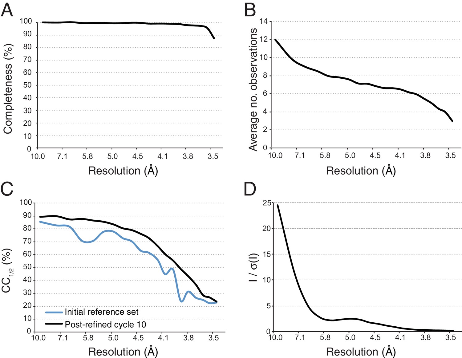
Statistical charts for scaled, merged and post-refined XFEL diffraction data.

(A) Completeness, (B) Average number of partial observations per Miller index, (C) CC_1/2, comparing the initial reference set and post-refined data set, (D) I / σ(I).

https://doi.org/10.7554/eLife.18740.015

Taken together, the improvements in XFEL processing methods resulted in better statistics for the XFEL diffraction data set of the Syt1–SNARE complex (Table 1) than previously published (Zhou et al., 2015). In particular, the reprocessed data set was is more complete (97.8% vs. 87.6%, respectively) than the previously published XFEL data set, has a higher multiplicity (6.1 vs. 5.0) and a better CC_1/2 (94.3% vs. 92.7%).

Effects of resolution and signal-to-noise cutoffs

Request a detailed protocol

We investigated the effects of applying different filters to the observed XFEL diffraction data prior to post-refinement and merging on the statistics of the merged data set: (a) merging with negative measurements (including all reflections with $I / σ (I) > - 3$ ); (b) merging using all reflections with $I / σ (I) > 0.5$ and omitting reflections higher than 4.1 Å Bragg spacings; and (c) merging using all reflections with $I / σ (I) > 0.5$ and omitting reflections lower than 10 Å Bragg spacings. Inclusion of the negative intensities slightly improved the merging and refinement statistics (Table 1), improved the L-test (Figure 4—figure supplement 2), and lowered the overall atomic model R values (Table 1). Omitting high- or low-resolution data has a small deleterious effect on the merging statistics (R_merge and CC_1/2) and the corresponding refined atomic models (Table 1), suggesting that the intensity measurements are of roughly the same quality throughout different resolutions. The electron density map generated from the XFEL data set that included negative intensities yielded higher average B-factor than that generated from the reflection set without negative intensities (~100 Å² vs. ~50 Å² respectively), but this had no substantial effect on the interpretability of the electron density maps, so the data set with negative intensities included was used for the final refinement of the Syt1–SNARE complex (Table 1).

In contrast to the substantial effect of excluding negative intensities on the L-test statistics of the observed XFEL data, the effect was very small for the simulated XFEL data (Figure 4—figure supplement 2). The effect on merging statistics and R-values of refined atomic models for the simulated XFEL data was similarly small (Table 1), likely due to the much smaller fraction of negative intensities in the simulated XFEL data (4.1%) than in the observed XFEL data (15.8%).

Synchrotron data collection and processing

Request a detailed protocol

Synchrotron data were collected using the shutterless, continuous rotation method at the Northeastern Collaborative Access Team (NE-CAT) beamline at the Advanced Photon Source at Argonne National Lab on a Pilatus 6M detector (Dectris). 80 cryo-cooled crystals were screened and the best diffraction data (in the long unit cell form) were merged from three data sets collected at three different positions on a single crystal using consecutive spindle angles. A 30 μm beam was used throughout the experiment. Each of the three data sets contained 150 diffraction images in 0.2° frames and an exposure time of 0.2 s. The diffraction images were indexed and integrated using XDS (Kabsch, 2010) and scaled and merged using Scala (Evans, 2006).

Atomic model refinements

Request a detailed protocol

The structure of the Syt1–SNARE complex was refined against the merged XFEL diffraction data set to 3.5 Å resolution (Table 1) in a manner similar to that previously described (Zhou et al., 2015). Briefly, the phases for the XFEL crystal structure of Syt1-SNARE complex were determined by molecular replacement with Phaser (McCoy, 2007) using the rat SNARE complex (PDB ID: 1N7S), the rat Syt1 C2A domain (PDB ID: 3F04), and the rat Syt1 C2B domain (PDB ID: 1UOW) as search models. The structure was iteratively rebuilt and initially refined using CNS v1.3 (Brunger et al., 1998), with deformable elastic network (DEN) restraints (Schroder et al., 2014), restrained grouped atomic displacement parameters (ADP) and non-crystallographic symmetry (NCS) restraints, then further refined with phenix.refine (Adams et al., 2010) using NCS restraints, secondary structure restraints, and individual ADP refinement. The unit cell dimensions for refinement were set to the mean values obtained by post-refinement with PRIME. Re-refinement of the Syt1 – SNARE structure against the reprocessed XFEL data resulted in better atomic model R_work / R_free values (29.2% / 32.9% vs. 32.2% / 35.3%) than the originally published structure. The final refinement cycle was replicated for the resolution- or intensity-truncated XFEL data sets (Table 1) in order to obtain comparable refinement statistics.

The phases for the synchrotron diffraction data were determined using molecular replacement and refined in the same manner as above. We transferred the test set of reflections for cross-validation that was used for the refinement against the XFEL data. Refined independently from the XFEL-data derived structure, the synchrotron data-derived structure yielded slightly better R_work / R_free values than the structure refined against the XFEL diffraction data truncated to the same resolution (4.1 Å) (Table 1).

Generation of simulated annealing composite omit maps

Request a detailed protocol

Composite omit maps were generated in order to reduce the potential effect of model bias (Figure 1—figure supplement 2). The maps were generated using phenix.composite_omit_map (Terwilliger et al., 2008) via the Phenix GUI (Echols et al., 2012), employing a single cycle of Cartesian simulated annealing (starting at 5000 K) to reduce model bias, followed by minimization. We chose to exclude bulk solvent from the omitted regions, as that option appeared to result in stronger omit map features.

Additional files

Request a detailed protocol

The merged XFEL diffraction data (Table 1A) and the merged synchrotron diffraction data (Table 1B) for the Syt1–SNARE complex, along with the corresponding atomic model coordinates have been deposited in the Protein Data Bank (PDB IDs 5KJ7 and 5KJ8, respectively). The merged simulated XFEL diffraction data (Table 1C) and corresponding atomic model coordinates are available as Source Data files. The complete set of raw XFEL diffraction images for the Syt1–SNARE complex will be deposited in the SBGrid data repository.

Data availability

The following data sets were generated

1. Lyubimov AY
2. Uervirojnangkoorn M
3. Zhou Q
4. Zhao M
5. Sauter NK
6. Brewster AS
7. Weis WI
8. Brunger AT
(2016) Raw XFEL diffraction images (MarCCD format) of Synaptotagmin-1 / SNARE complex, associated with PDB entry 5KJ7
Publicly available at the Structural Biology Data Grid.

http://dx.doi.org/10.15785/SBGRID/365
1. Lyubimov AY
2. Uervirojnangkoorn M
3. Zhou Q
4. Zhao M
5. Sauter NK
6. Brewster AS
7. Weis WI
8. Brunger AT
(2016) Structure of the Ca2+-bound synaptotagmin-1 SNARE complex (long unit cell form) - from XFEL diffraction
Publicly available at the RCSB Protein Data Bank (accession no: 5KJ7).

http://www.rcsb.org/pdb/explore/explore.do?structureId=5KJ7
1. Lyubimov AY
2. Uervirojnangkoorn M
3. Zhou Q
4. Zhao M
5. Sauter NK
6. Brewster AS
7. Weis WI
8. Brunger AT
(2016) Structure of the Ca2+-bound synaptotagmin-1 SNARE complex (long unit cell form) - from synchrotron diffraction
Publicly available at the RCSB Protein Data Bank (accession no: 5KJ8).

http://www.rcsb.org/pdb/explore/explore.do?structureId=5KJ8

References

1. Adams PD
2. Afonine PV
3. Bunkóczi G
4. Chen VB
5. Davis IW
6. Echols N
7. Headd JJ
8. Hung LW
9. Kapral GJ
10. Grosse-Kunstleve RW
11. McCoy AJ
12. Moriarty NW
13. Oeffner R
14. Read RJ
15. Richardson DC
16. Richardson JS
17. Terwilliger TC
18. Zwart PH
(2010) PHENIX: a comprehensive Python-based system for macromolecular structure solution
Acta Crystallographica. Section D, Biological Crystallography 66:213–221.
https://doi.org/10.1107/S0907444909052925
- PubMed
- Google Scholar
1. Amann J
2. Berg W
3. Blank V
4. Decker F-J
5. Ding Y
6. Emma P
7. Feng Y
8. Frisch J
9. Fritz D
10. Hastings J
11. Huang Z
12. Krzywinski J
13. Lindberg R
14. Loos H
15. Lutman A
16. Nuhn H-D
17. Ratner D
18. Rzepiela J
19. Shu D
20. Shvyd'ko Y
21. Spampinati S
22. Stoupin S
23. Terentyev S
24. Trakhtenberg E
25. Walz D
26. Welch J
27. Wu J
28. Zholents A
29. Zhu D
(2012) Demonstration of self-seeding in a hard-X-ray free-electron laser
Nature Photonics 6:693–698.
https://doi.org/10.1038/nphoton.2012.180
- Google Scholar
1. Andrews LC
2. Bernstein HJ
(2014) The geometry of Niggli reduction: BGAOL -embedding Niggli reduction and analysis of boundaries
Journal of Applied Crystallography 47:346–359.
https://doi.org/10.1107/S1600576713031002
- PubMed
- Google Scholar
(1994) Spectrum, temporal structure, and fluctuations in a high-gain free-electron laser starting from noise
Physical Review Letters 73:70–73.
https://doi.org/10.1103/PhysRevLett.73.70
- PubMed
- Google Scholar
1. Brünger AT
2. Adams PD
3. Clore GM
4. DeLano WL
5. Gros P
6. Grosse-Kunstleve RW
7. Jiang JS
8. Kuszewski J
9. Nilges M
10. Pannu NS
11. Read RJ
12. Rice LM
13. Simonson T
14. Warren GL
(1998) Crystallography & NMR system: A new software suite for macromolecular structure determination
Acta Crystallographica. Section D, Biological Crystallography 54:905–921.
https://doi.org/10.1107/s0907444998003254
- PubMed
- Google Scholar
(2002) An automated system to mount cryo-cooled protein crystals on a synchrotron beam line, using compact sample cassettes and a small-scale robot
Journal of Applied Crystallography 35:720–726.
https://doi.org/10.1107/S0021889802016709
- PubMed
- Google Scholar
1. Cohen AE
2. Soltis SM
3. González A
4. Aguila L
5. Alonso-Mori R
6. Barnes CO
7. Baxter EL
8. Brehmer W
9. Brewster AS
10. Brunger AT
11. Calero G
12. Chang JF
13. Chollet M
14. Ehrensberger P
15. Eriksson TL
16. Feng Y
17. Hattne J
18. Hedman B
19. Hollenbeck M
20. Holton JM
21. Keable S
22. Kobilka BK
23. Kovaleva EG
24. Kruse AC
25. Lemke HT
26. Lin G
27. Lyubimov AY
28. Manglik A
29. Mathews II
30. McPhillips SE
31. Nelson S
32. Peters JW
33. Sauter NK
34. Smith CA
35. Song J
36. Stevenson HP
37. Tsai Y
38. Uervirojnangkoorn M
39. Vinetsky V
40. Wakatsuki S
41. Weis WI
42. Zadvornyy OA
43. Zeldin OB
44. Zhu D
45. Hodgson KO
(2014) Goniometer-based femtosecond crystallography with X-ray free electron lasers
PNAS 111:17122–17127.
https://doi.org/10.1073/pnas.1418733111
- PubMed
- Google Scholar
(2012) Graphical tools for macromolecular crystallography in PHENIX
Journal of Applied Crystallography 45:581–586.
https://doi.org/10.1107/S0021889812017293
- PubMed
- Google Scholar
1. Emma P
2. Akre R
3. Arthur J
4. Bionta R
5. Bostedt C
6. Bozek J
7. Brachmann A
8. Bucksbaum P
9. Coffee R
10. Decker F-J
11. Ding Y
12. Dowell D
13. Edstrom S
14. Fisher A
15. Frisch J
16. Gilevich S
17. Hastings J
18. Hays G
19. Hering P
20. Huang Z
21. Iverson R
22. Loos H
23. Messerschmidt M
24. Miahnahri A
25. Moeller S
26. Nuhn H-D
27. Pile G
28. Ratner D
29. Rzepiela J
30. Schultz D
31. Smith T
32. Stefan P
33. Tompkins H
34. Turner J
35. Welch J
36. White W
37. Wu J
38. Yocky G
39. Galayda J
(2010) First lasing and operation of an ångstrom-wavelength free-electron laser
Nature Photonics 4:641–647.
https://doi.org/10.1038/nphoton.2010.176
- Google Scholar
1. Evans P
(2006) Scaling and assessment of data quality
Acta Crystallographica. Section D, Biological Crystallography 62:72–82.
https://doi.org/10.1107/S0907444905036693
- PubMed
- Google Scholar
1. Ginn HM
2. Brewster AS
3. Hattne J
4. Evans G
5. Wagner A
6. Grimes JM
7. Sauter NK
8. Sutton G
9. Stuart DI
(2015a) A revised partiality model and post-refinement algorithm for X-ray free-electron laser data
Acta Crystallographica. Section D, Biological Crystallography 71:1400–1410.
https://doi.org/10.1107/S1399004715006902
- PubMed
- Google Scholar
1. Ginn HM
2. Messerschmidt M
3. Ji X
4. Zhang H
5. Axford D
6. Gildea RJ
7. Winter G
8. Brewster AS
9. Hattne J
10. Wagner A
11. Grimes JM
12. Evans G
13. Sauter NK
14. Sutton G
15. Stuart DI
(2015b) Structure of CPV17 polyhedrin determined by the improved analysis of serial femtosecond crystallographic data
Nature Communications 6:6435.
https://doi.org/10.1038/ncomms7435
- Google Scholar
1. Hattne J
2. Echols N
3. Tran R
4. Kern J
5. Gildea RJ
6. Brewster AS
7. Alonso-Mori R
8. Glöckner C
9. Hellmich J
10. Laksmono H
11. Sierra RG
12. Lassalle-Kaiser B
13. Lampe A
14. Han G
15. Gul S
16. DiFiore D
17. Milathianaki D
18. Fry AR
19. Miahnahri A
20. White WE
21. Schafer DW
22. Seibert MM
23. Koglin JE
24. Sokaras D
25. Weng TC
26. Sellberg J
27. Latimer MJ
28. Glatzel P
29. Zwart PH
30. Grosse-Kunstleve RW
31. Bogan MJ
32. Messerschmidt M
33. Williams GJ
34. Boutet S
35. Messinger J
36. Zouni A
37. Yano J
38. Bergmann U
39. Yachandra VK
40. Adams PD
41. Sauter NK
(2014) Accurate macromolecular structures using minimal measurements from X-ray free-electron lasers
Nature Methods 11:545–548.
https://doi.org/10.1038/nmeth.2887
- PubMed
- Google Scholar
1. Helliwell JR
2. Greenhough TJ
3. Carr PD
4. Rule SA
5. Moore PR
6. Thompson AW
7. Worgan JS
(1982) Central data collection facility for protein crystallography, small angle diffraction and scattering at the Daresbury Laboratory Synchrotron Radiation Source (SRS), England
Journal of Physics E: Scientific Instruments 15:1363–1372.
https://doi.org/10.1088/0022-3735/15/12/023
- Google Scholar
1. Hirata K
2. Shinzawa-Itoh K
3. Yano N
4. Takemura S
5. Kato K
6. Hatanaka M
7. Muramoto K
8. Kawahara T
9. Tsukihara T
10. Yamashita E
11. Tono K
12. Ueno G
13. Hikima T
14. Murakami H
15. Inubushi Y
16. Yabashi M
17. Ishikawa T
18. Yamamoto M
19. Ogura T
20. Sugimoto H
21. Shen JR
22. Yoshikawa S
23. Ago H
(2014) Determination of damage-free crystal structure of an X-ray-sensitive protein using an XFEL
Nature Methods 11:734–U174.
https://doi.org/10.1038/nmeth.2962
- PubMed
- Google Scholar
(2012) The point-spread function of fiber-coupled area detectors
Journal of Synchrotron Radiation 19:1006–1011.
https://doi.org/10.1107/S0909049512035571
- PubMed
- Google Scholar
1. Kabsch W
(2010) XDS
Acta Crystallographica. Section D, Biological Crystallography 66:125–132.
https://doi.org/10.1107/S0907444909047337
- PubMed
- Google Scholar
1. Kabsch W
(2014) Processing of X-ray snapshots from crystals in random orientations
Acta Crystallographica. Section D, Biological Crystallography 70:2204–2216.
https://doi.org/10.1107/S1399004714013534
- PubMed
- Google Scholar
1. Kern J
2. Alonso-Mori R
3. Hellmich J
4. Tran R
5. Hattne J
6. Laksmono H
7. Glockner C
8. Echols N
9. Sierra RG
10. Sellberg J
11. Lassalle-Kaiser B
12. Gildea RJ
13. Glatzel P
14. Grosse-Kunstleve RW
15. Latimer MJ
16. McQueen TA
17. DiFiore D
18. Fry AR
19. Messerschmidt M
20. Miahnahri A
21. Schafer DW
22. Seibert MM
23. Sokaras D
24. Weng T-C
25. Zwart PH
26. White WE
27. Adams PD
28. Bogan MJ
29. Boutet S
30. Williams GJ
31. Messinger J
32. Sauter NK
33. Zouni A
34. Bergmann U
35. Yano J
36. Yachandra VK
(2012) Room temperature femtosecond X-ray diffraction of photosystem II microcrystals
PNAS 109:9721–9726.
https://doi.org/10.1073/pnas.1204598109
- Google Scholar
1. Kirian RA
2. Wang X
3. Weierstall U
4. Schmidt KE
5. Spence JC
6. Hunter M
7. Fromme P
8. White T
9. Chapman HN
10. Holton J
(2010) Femtosecond protein nanocrystallography-data analysis methods
Optics Express 18:5713–5723.
https://doi.org/10.1364/OE.18.005713
- PubMed
- Google Scholar
(2015) Accounting for partiality in serial crystallography using ray-tracing principles
Acta Crystallographica. Section D, Biological Crystallography 71:1799–1811.
https://doi.org/10.1107/S1399004715011803
- PubMed
- Google Scholar
1. Lyubimov AY
2. Murray TD
3. Koehl A
4. Araci IE
5. Uervirojnangkoorn M
6. Zeldin OB
7. Cohen AE
8. Soltis SM
9. Baxter EL
10. Brewster AS
11. Sauter NK
12. Brunger AT
13. Berger JM
(2015) Capture and X-ray diffraction studies of protein microcrystals in a microfluidic trap array
Acta Crystallographica. Section D, Biological Crystallography 71:928–940.
https://doi.org/10.1107/S1399004715002308
- PubMed
- Google Scholar
(2016) IOTA: integration optimization, triage and analysis tool for the processing of XFEL diffraction images
Journal of Applied Crystallography 49:1057–1064.
https://doi.org/10.1107/S1600576716006683
- PubMed
- Google Scholar
1. McCoy AJ
(2007) Solving structures of protein complexes by molecular replacement with Phaser
Acta Crystallographica. Section D, Biological Crystallography 63:32–41.
https://doi.org/10.1107/S0907444906045975
- PubMed
- Google Scholar
(2015) A high-transparency, micro-patternable chip for X-ray diffraction analysis of microcrystals under native growth conditions
Acta Crystallographica. Section D, Biological Crystallography 71:1987–1997.
https://doi.org/10.1107/S1399004715015011
- PubMed
- Google Scholar
1. Padilla JE
2. Yeates TO
(2003) A statistic for local intensity differences: robustness to anisotropy and pseudo-centering and utility for detecting twinning
Acta Crystallographica Section D Biological Crystallography 59:1124–1130.
https://doi.org/10.1107/S0907444903007947
- PubMed
- Google Scholar
(2004) Robust indexing for automatic data collection
Journal of Applied Crystallography 37:399–409.
https://doi.org/10.1107/S0021889804005874
- PubMed
- Google Scholar
(2006) Improved statistics for determining the Patterson symmetry from unmerged diffraction intensities
Journal of Applied Crystallography 39:158–168.
https://doi.org/10.1107/S0021889805042299
- Google Scholar
1. Sauter NK
2. Hattne J
3. Brewster AS
4. Echols N
5. Zwart PH
6. Adams PD
(2014) Improved crystal orientation and physical properties from single-shot XFEL stills
Acta Crystallographica. Section D, Biological Crystallography 70:3299–3309.
https://doi.org/10.1107/S1399004714024134
- PubMed
- Google Scholar
1. Sauter NK
(2015) XFEL diffraction: developing processing methods to optimize data quality
Journal of Synchrotron Radiation 22:239–248.
https://doi.org/10.1107/S1600577514028203
- PubMed
- Google Scholar
1. Schlichting I
(2015) Serial femtosecond crystallography: the first five years
IUCrJ 2:246–255.
https://doi.org/10.1107/S205225251402702X
- PubMed
- Google Scholar
(2014) Deformable elastic network refinement for low-resolution macromolecular crystallography
Acta Crystallographica. Section D, Biological Crystallography 70:2241–2255.
https://doi.org/10.1107/S1399004714016496
- PubMed
- Google Scholar
1. Suga M
2. Akita F
3. Hirata K
4. Ueno G
5. Murakami H
6. Nakajima Y
7. Shimizu T
8. Yamashita K
9. Yamamoto M
10. Ago H
11. Shen JR
(2015) Native structure of photosystem II at 1.95 Å resolution viewed by femtosecond X-ray pulses
Nature 517:99–103.
https://doi.org/10.1038/nature13991
- PubMed
- Google Scholar
(2008) Iterative-build OMIT maps: map improvement by iterative model building and refinement without model bias
Acta Crystallographica. Section D, Biological Crystallography 64:515–524.
https://doi.org/10.1107/S0907444908004319
- PubMed
- Google Scholar
(2015) Enabling X-ray free electron laser crystallography for challenging biological systems from a limited number of crystals
eLife 4:e05421.
https://doi.org/10.7554/eLife.05421
- PubMed
- Google Scholar
1. Waterman DG
2. Winter G
3. Gildea RJ
4. Parkhurst JM
5. Brewster AS
6. Sauter NK
7. Evans G
(2016) Diffraction-geometry refinement in the DIALS framework
Acta Crystallographica. Section D, Structural Biology 72:558–575.
https://doi.org/10.1107/S2059798316002187
- PubMed
- Google Scholar
1. White TA
(2014) Post-refinement method for snapshot serial crystallography
Philosophical Transactions of the Royal Society B: Biological Sciences 369:20130330.
https://doi.org/10.1098/rstb.2013.0330
- Google Scholar
1. Young ID
2. Ibrahim M
3. Chatterjee R
4. Gul S
5. Fuller F
6. Koroidov S
7. Brewster AS
8. Tran R
9. Alonso-Mori R
10. Kroll T
11. Michels-Clark T
12. Laksmono H
13. Sierra RG
14. Stan CA
15. Hussein R
16. Zhang M
17. Douthit L
18. Kubin M
19. de Lichtenberg C
20. Pham LV
21. Nilsson H
22. Cheah MH
23. Shevela D
24. Saracini C
25. Bean MA
26. Seuffert I
27. Sokaras D
28. Weng T-C
29. Pastor E
30. Weninger C
31. Fransson T
32. Lassalle L
33. Bräuer P
34. Aller P
35. Docker PT
36. Andi B
37. Orville AM
38. Glownia JM
39. Nelson S
40. Sikorski M
41. Zhu D
42. Hunter MS
43. Lane TJ
44. Aquila A
45. Koglin JE
46. Robinson J
47. Liang M
48. Boutet S
49. Lyubimov AY
50. Uervirojnangkoorn M
51. Moriarty NW
52. Liebschner D
53. Afonine PV
54. Waterman DG
55. Evans G
56. Wernet P
57. Dobbek H
58. Weis WI
59. Brunger AT
60. Zwart PH
61. Adams PD
62. Zouni A
63. Messinger J
64. Bergmann U
65. Sauter NK
66. Kern J
67. Yachandra VK
68. Yano J
(2016)
Structure of photosystem II and substrate binding at room temperature

Nature.
- Google Scholar
1. Zeldin OB
2. Brewster AS
3. Hattne J
4. Uervirojnangkoorn M
5. Lyubimov AY
6. Zhou Q
7. Zhao M
8. Weis WI
9. Sauter NK
10. Brunger AT
(2015) Data Exploration Toolkit for serial diffraction experiments
Acta Crystallographica. Section D, Biological Crystallography 71:352–356.
https://doi.org/10.1107/S1399004714025875
- PubMed
- Google Scholar
1. Zhou Q
2. Lai Y
3. Bacaj T
4. Zhao M
5. Lyubimov AY
6. Uervirojnangkoorn M
7. Zeldin OB
8. Brewster AS
9. Sauter NK
10. Cohen AE
11. Soltis SM
12. Alonso-Mori R
13. Chollet M
14. Lemke HT
15. Pfuetzner RA
16. Choi UB
17. Weis WI
18. Diao J
19. Südhof TC
20. Brunger AT
(2015) Architecture of the synaptotagmin-SNARE machinery for neuronal exocytosis
Nature 525:62–67.
https://doi.org/10.1038/nature14975
- PubMed
- Google Scholar
(2006) Exploring metric symmetry
CCP4 Newsletter.
https://doi.org/10.2172/926901
- Google Scholar

Decision letter

Stephen C. Harrison

Reviewing Editor; Harvard Medical School, United States

In the interests of transparency, eLife includes the editorial decision letter and accompanying author responses. A lightly edited version of the letter sent to the authors after peer review is shown, indicating the most substantive concerns; minor comments are not usually included.

Thank you for submitting your article "Advances in XFEL diffraction data processing applied to the crystal structure of the synaptotagmin-1 / SNARE complex" for consideration by eLife. Your article has been favorably evaluated by Arup Chakraborty as the Senior Editor and three reviewers, including Tom Terwilliger (Reviewer #2) and Stephen C. Harrison (Reviewer #1), who is a member of our Board of Reviewing Editors.

The reviewers have discussed the reviews with one another and the Reviewing Editor has drafted this decision to help you prepare a revised submission.

Summary:

This is a Research Advance that indeed reports improvements in the software previously described in eLife (Uevirojnankoorn et al., 2015) and that comes to updated conclusions. It thus conforms appropriately to the intent of the Research Advance category and merits publication.

The authors have made some substantial changes to their approach for analyzing the still images obtained from XFEL data. The new approaches allow treatment of reflections with negative intensities and the use of pseudo-Wilson scaling to normalize not just the average intensity of each image but also the fall-off with resolution (as has been done as a matter of course previously for synchrotron data but not for XFEL data). These approaches were applied to previously analyzed data for a synaptotagmin/SNARE complex, and the resulting maps appear to show more detail than those calculated with data treated by the earlier methods. Moreover, density correlations were better for the XFEL maps than for maps from synchrotron data from similar crystals.

Essential revisions:

Attention to the suggestions (a) and (b) under (1) and to one or more of the suggestions (i), (ii), and (iii) under (2)(b) would make the paper stronger; those calculations should be straightforward and take relatively little time. Many of the other points raised here cannot be settled with the current data, but some comments on those points would be valuable.

1) Improvement from reprocessing XFEL data. The data from the reprocessing are more complete (98% vs. 88%), but a large fraction have negative intensities, and excluding the negative intensities reduces the completeness to 88%, the same as for the previous analysis. The CC_1/2 is marginally better (94% vs. 93%) for the reprocessed data. The free R value for the complex was lower for the reprocessed data (33% vs. 35%). This is the most convincing evidence that the reprocessed data are more accurate, but as the models were not the same, it is not easy to tell if the change is significant.

Suggestions:

a) It would be helpful to show a detailed comparison of the previous XFEL data with the current data. For example, what is the correlation of intensities between previous and current processed data, and what is the I/σ vs. resolution for each, after selecting the data that are in common between the two?

b) It would also be helpful to refine the same model against the previous and current XFEL datasets, only adjusting parameter values, to have a more convincing comparison based on decrease in the free R.

2) Comparison with synchrotron source. The R-factor and other formal comparisons of the model refinement suggest that the model fits the synchrotron dataset more closely, even when allowing for the resolution difference. This conflict between the free R (overall agreement between model and data) and the real-space correlation (average local agreement between model and data) is unusual. Thus, there appear to be two key issues at this point, neither related to whether the software needs even more work. (a) One key issue, which the authors cannot settle with the current data – if they could, this would be a new paper, not an Advance – appears to be: what is the physical explanation for the differences in the data sets? Excluding for now potentially undiscovered aspects of the scattering physics from the intense XFEL beam, one can see at least three reasons why the data might be different: (i) differences in the way data were collected and merged; (ii) differences in crystal damage (including, of course, the possibility that there was very little in the XFEL case); (iii) differences in the crystals themselves on the two occasions, separated substantially in time. (b) The other key issue is: why does an atomic model fit one better than the other? A hypothesis that needs testing is that the 2F_o-F_c map calculated from the XFEL dataset has more model bias because of less accurate data. (The rationale behind this hypothesis is that a dataset with zero I/σ everywhere would effectively look just like the model because the 2(F_o-F_c) portion of the 2F_o-F_c map would be random and the F_o portion would look just like the model).

a) What is the physical explanation for the differences in the data sets?i) The single-crystal data came from three fixed positions, with ccd recording. Current experience shows that this regime gives less accurate intensities than the continuous motion regime made possible by direct x-ray detectors. The latter strategy yields data with more uniform B-factors (instead of a "sawtooth" dependence of B-factor on frame number) and more favorable statistics. Nonetheless, a single crystal is more likely than many crystals to have essentially identical unit-cell contents, packing, etc., from one place to another than will a large number of crystals, and perhaps it is not surprising that despite the greater "blur" (higher net B, etc.), one model fits that set better than it does a set merged from many crystals.

ii) It might be a good idea to include the "sawtooth" B-versus-frame number plot for the single crystals, to show how much damage resulted from the total exposure at each location. Did the initial frames show measurable Bragg intensities beyond 4.1 Å? If so, the right comparison of synchrotron and XFEL might have been, for the former case, to collect only as many frames from each position that showed no evident decay, if necessary using more than one crystal to complete the data (but of course getting into an issue of crystal-to-crystal variation – perhaps minimized by taking crystals from a single drop).

iii) With two molecular complexes in the asymmetric unit, there are probably more possibilities for batch-to-batch variation (let alone one year to the next variation) from many small crystals than with just a couple of much larger ones.

b) Why does an atomic model fit one better than the other? Some possible tests for model bias and related issues are suggested below.

i) Calculate a composite omit map (with refinement) instead of a 2F_o-F_c map and analyze this map. For example one could do this by: (1) adjusting the Wilson B of the synchrotron and XFEL datasets to the same value. (j2) removing anisotropy, (3) setting the cell constants of the two datasets to both be equal to the APS dataset, (4) refining the APS model against both datasets, (5) calculating the refined composite omit map, and (6) comparing the map to the model. When one of the reviewers (TT) did this, he found adjusting the cell dimensions didn't change the Rfree for the XFEL dataset very much (R_free=0.34 compared to 0.33 using original cell parameters). He obtained very similar correlations of XFEL and APS composite omit maps to their respective refined models in the region of the models (0.75 for XFEL vs. 0.74 for APS). The correlation calculated over the entire unit cell was somewhat better for the APS data (0.62 vs. 0.59). This result would suggest that the APS data are at least as accurate as the XFEL data.

ii) Calculate a F_o(XFEL) – F_o(synchrotron) map phased with model phases (either model). This again requires the assumption of equal cell dimensions. This map should show differences between the density corresponding to the two datasets and would be expected to have peaks at positions of side chains that are radiation sensitive (or perhaps at sulfur positions). TT calculated such a map and could not see any such pattern of density in the map (it looked almost random but not quite as there were more peaks in the protein region than in the solvent). This did not provide any evidence for a systematic difference between the two datasets at positions of radiation-sensitive atoms. It is possible that the cell dimensions really are different, affecting the difference map (although the similar free R value obtained above with different cell dimensions would argue against this interpretation).

iii) Calculate correlation or R-values of data from APS data collected at lower dose or higher dose with XFEL data. This could be done by processing just early frames of APS data or just late frames of this data and comparing each to the XFEL data. If radiation damage is less in the XFEL data it might be expected to correlate better with the early APS data (though other interpretations would still be possible). See also (a)(ii), above.

The authors suggest that the XFEL dataset had less radiation damage because the correlation difference was bigger for those side chains known to be more sensitive to radiation damage. But among the 7 side chains with the largest differences, four (Gly, Lys, Ser and Gln) are not thought to be sensitive, while Glu, one of the most sensitive, is only 13th in the sorted list. Are the Cys residues involved in di-sulfide bridges? These are far more sensitive than a cysteine. Thus, it seems likely that, while radiation damage may be a contributing factor to the observed differences, it is not the whole story.

In summary, the new software is an advance, but the reviewers are not convinced by the second conclusion – which is in any case not needed to qualify for a Research Advance publication – that "XFELs can improve upon the data obtained from synchrotrons". It has clearly done so (somewhat marginally, but nonetheless properly documented here, including the local real-space correlations, etc.) for this particular synchrotron data set, but the thoughts just outlined illustrate why that data set might not have been optimal and why the comparison may to some extent be apples and oranges.

Thus, the authors should revise the text to avoid conclusions about data "quality" and rather should focus on what this Advance is really about anyway – the new algorithms and software that implements them. To the extent that comparison with synchrotron and simulated data allows them to assess the new methods, inclusion of those comparisons is excellent. But avoid comparing what cannot, at this stage, be properly compared.

https://doi.org/10.7554/eLife.18740.026

Author response

[…] Essential revisions:

1) Improvement from reprocessing XFEL data. The data from the reprocessing are more complete (98% vs. 88%), but a large fraction have negative intensities, and excluding the negative intensities reduces the completeness to 88%, the same as for the previous analysis. The CC_1/2is marginally better (94% vs. 93%) for the reprocessed data. The free R value for the complex was lower for the reprocessed data (33% vs. 35%). This is the most convincing evidence that the reprocessed data are more accurate, but as the models were not the same, it is not easy to tell if the change is significant.

We agree that the relative improvement due to the reprocessing of the XFEL diffraction data was modest. This was as expected, as the reprocessing was carried out mostly to account for the changes and improvements in the processing software. We believe that the original XFEL-derived structure of Syt1-SNARE was refined with sufficiently good R-values and geometry to merit publication and deposition to the Protein Data Bank.

We would like to clarify that the improvements to the data processing software came in two installments. The first installment (comprising improvements to the software since the publication of articles describing the software) included changes in cctbx.xfel in how the lattice model is generated (specifically concerning the transition from triclinic to higher-symmetry Bravais lattice) as well as the implementation of the pseudo-Wilson scaling in PRIME. These changes were made while the original Syt1-SNARE structure was being refined against XFEL diffraction data. They resulted in the structure published by (Zhou et al., 2015). After the publication of that structure, further changes were made to the software, which resulted in additional improvements to the electron density maps and refined atomic model of the Syt1-SNARE complex described in this Research Advance.

We have added additional details in the Results section of the manuscript, clarifying which changes applied to which version of the Syt1-SNARE XFEL structure. We have also added a new figure supplement to provide an example of the improvements in the atomic model made possible by the most recent methods development (new Figure 1—figure supplement 1).

Suggestions:

Comparison of the originally-processed (“old”) and re-processed (“new”) XFEL datasets using the reflections in common shows a significant drop in correlation after ~4.3 Å (Author response image 1). These results suggest that the improved XFEL diffraction data processing techniques reported here most strongly affected the high-resolution diffraction data.

Author response image 1

Download asset Open asset

Statistical analysis of XFEL diffraction dataset reprocessing.

Correlation coefficients (red line) and R-values (blue line) between original and reprocessed XFEL diffraction datasets.

https://doi.org/10.7554/eLife.18740.017

We performed bulk solvent and anisotropic scaling refinement of the new XFEL Syt1-SNARE structure reported here (PDB ID: 5KJ7) against the originally published XFEL dataset resulting in R_work = 31.1% and R_free = 33.6%. When only reflections with positive measurements were included in the reprocessed XFEL diffraction dataset, both R_work and R_free were 1.1% and 0.4% lower, respectively, than those for the original XFEL diffraction data. Inclusion of negative intensity measurements further lowered the overall R_work and R_free values by 0.8% and 0.3%, respectively, for the reprocessed data. These observations indicate that the reprocessing produces data that give somewhat more accurate models. The improved completeness provided by including negative data may also help in this regard. We have added this point to the text.

Please note that the electron density maps presented in Figure 1 are σ_A weighted. This technique effectively down weights the weak data in high resolution shells when generating the maps and minimizes potential model bias. Moreover, as we now document more carefully in the revised manuscript (new Figure 1—figure supplement 1), the 2mF_o-DF_c electron density maps derived from the XFEL diffraction data reveal features not seen in the synchrotron-data derived maps. For example, some side chain rotamers had to be adjusted (or, in some cases, modeled for the first time) in the XFEL-data derived maps. Thus, we conclude that the features revealed by the XFEL-data derived electron density maps are not likely the result of model bias. The composite omit maps calculated with simulated annealing to alleviate model bias (new Figure 1—figure supplement 2) support this assertion.

The synchrotron diffraction data for Syt1-SNARE were collected using a Dectris Pilatus 6M detector in a shutterless, continuous rotation mode with 0.2° frames (we have added this detail to the Methods section of the manuscript). We agree that variation in unit cell parameters, diffraction strength due to pulse intensity and crystal size differences are likely to give rise to differences with the single crystal diffraction data. We have added this detail to the Results and Discussion section of the manuscript.

ii) It might be a good idea to include the "sawtooth" B-versus-frame number plot for the single crystals, to show how much damage resulted from the total exposure at each location.

The R_d plots, provided by the XDS package as a crude measure of radiation damage (Diederichs, 2006), show a clear effect vs. exposure (Author response image 2A–C). This suggests that synchrotron data collection resulted in noticeable radiation damage to the crystal despite the care that was taken to minimize it.

Author response image 2

Download asset Open asset

Analysis of radiation damage effect on synchrotron diffraction data.

(A–C) R_d plot vs. Φ angle for diffraction data collected at three separate positions on the same Syt1-SNARE crystal. Colored boxes represent sub-datasets (green – first 1/3 of the dataset, red – mid 1/3 of the dataset, blue – last 1/3 of the dataset). (D) R-factors between the full XFEL diffraction dataset and the three synchrotron sub-datasets; (E) Correlation coefficients between the two datasets. The colors for (D) and (E) follow the same scheme as that of (A–C); the full synchrotron dataset is shown as a black line.

https://doi.org/10.7554/eLife.18740.018

The R_d plots also demonstrate why multi-volume diffraction data collection was needed in this case, and suggests that a serial data collection approach – such as one used in our XFEL experiment – might improve upon synchrotron diffraction data.

Did the initial frames show measurable Bragg intensities beyond 4.1 Å? If so, the right comparison of synchrotron and XFEL might have been, for the former case, to collect only as many frames from each position that showed no evident decay, if necessary using more than one crystal to complete the data (but of course getting into an issue of crystal-to-crystal variation – perhaps minimized by taking crystals from a single drop).

Visual inspection of the synchrotron Syt1-SNARE diffraction images shows very weak reflections at ~3.8 – 4.0 Å in the first few images. However, such higher resolution reflections are not visible anymore in subsequent images.

Nevertheless, we attempted to merge the synchrotron diffraction data to beyond 4.1 Å, and noticed a sudden, precipitous deterioration of CC_1/2, R_meas and I / σ(I) in the resolution shells past that threshold. Attempts to match the 3.5 Å resolution of the XFEL data set resulted in even poorer merging statistics, indicating the lack of any interpretable diffraction at that resolution. Therefore, we believe that we cannot extend the resolution of the synchrotron diffraction dataset past 4.1 Å.

We agree that this is definitely possible and have added this point to the Results and Discussion portion of the text.

b) Why does an atomic model fit one better than the other? Some possible tests for model bias and related issues are suggested below.

i) Calculate a composite omit map (with refinement) instead of a 2F_o-F_c map and analyze this map. For example one could do this by: (1) adjusting the Wilson B of the synchrotron and XFEL datasets to the same value. (2) removing anisotropy, (3) setting the cell constants of the two datasets to both be equal to the APS dataset, (4) refining the APS model against both datasets, (5) calculating the refined composite omit map, and (6) comparing the map to the model. When one of the reviewers (TT) did this, he found adjusting the cell dimensions didn't change the Rfree for the XFEL dataset very much (R_free=0.34 compared to 0.33 using original cell parameters). He obtained very similar correlations of XFEL and APS composite omit maps to their respective refined models in the region of the models (0.75 for XFEL vs. 0.74 for APS). The correlation calculated over the entire unit cell was somewhat better for the APS data (0.62 vs. 0.59). This result would suggest that the APS data are at least as accurate as the XFEL data.

We have calculated two types of composite omit maps: 1) A “refined” (as per definition in the phenix GUI, not involving simulated annealing) composite omit map suggested in item (5) above, though matching each dataset with the model that was refined against it, rather than using the same model for all calculations; 2) A simulated-annealing composite omit map (with bulk solvent excluded from the omitted regions as implemented in phenix). To facilitate comparison, we calculated omit maps for both the XFEL and synchrotron datasets. In addition, we \ calculated such maps for the XFEL dataset truncated to 4.1 Å and for the “sharpened” synchrotron dataset, with the Wilson B-factor matching that of the XFEL dataset.

For the refined composite omit maps, we obtained similar results to the reviewer, in that the global real-space correlation coefficients (CCs) were fairly similar between the various datasets used. However, the real-space CCs per residue type shows a compelling overall pattern: the 3.5 Å XFEL data usually gave the highest CCs, while truncating the resolution to 4.1 Å yielded similar CCs than the synchrotron data set. Sharpening the synchrotron data had little effect. For individual Ca²⁺ ions, the XFEL datasets have yielded higher CCs in more than half of the cases. For the simulated-annealing composite omit maps (new Figure 1—figure supplement 2), CCs per residue group and for Ca²⁺ ions showed more pronounced differences, with the XFEL data yielding higher CCs in virtually all cases. The resolution effect persists across the board (new Figure 2—figure supplement 1). We have added these points to the text. We included the simulated annealing composite omit maps in this manuscript (new Figure 1—figure supplement 2).

We believe that an F_o-F_o analysis would not be very informative due to crystal and unit cell variability and potential scaling issues between the data sets that would introduce large difference features obscuring the differences in side chain densities.

For this analysis, we used the synchrotron sub-datasets collected for the three diffraction volumes of the chosen crystal; each of these datasets contained 150 diffraction images, which were separated into three subsets (“first 1/3 of the dataset”, “mid 1/3 of the dataset” and “last 1/3 of the dataset”). We then generated merged datasets for each “time point” by merging the 50-frame (10°) subsets from all three diffraction volumes (Author response image 2A–C). While this analysis is useful for addressing the reviewer’s suggestion we believe that it does not pertain to the key messages of this Research Advance so have not included it in the revised manuscript.

Calculating the R-values between the XFEL diffraction dataset and the three sub-datasets also reveals a clear dose effect, predominantly beyond ~ 4.6 Å, where the last 50 images have worse R-values vs. XFEL diffraction data than the mid-50 images and far worse R-values than the first 50 images (Author response image 2D). The plot of the correlation coefficients of the same sub-datasets shows something similar, albeit to a lesser extent (Author response image 2E).

None of the Cys residues are involved in disulfide bridges; furthermore, as steps were taken to minimize radiation damage (specifically, the multi-volume diffraction data collection strategy), we do not expect the effects to be particularly severe. We do agree with the reviewers that radiation damage, while a contributing factor, is not the whole story. We have modified the text accordingly.

We agree and have revised the text to avoid the appearance of implying that we have conclusively shown that “XFELs can improve upon the data obtained from synchrotrons”. This will be the subject of future investigations.

We thank the referees for a thorough review and have modified the manuscript accordingly.

https://doi.org/10.7554/eLife.18740.027

Article and author information

Author details

Artem Y Lyubimov
1. Department of Molecular and Cellular Physiology, Stanford University, Stanford, United States
2. Neurology and Neurological Science, Stanford University, Stanford, United States
3. Structural Biology, Stanford University, Stanford, United States
4. Photon Science, Stanford University, Stanford, United States
5. Howard Hughes Medical Institute, Stanford University, Stanford, United States
Contribution
AYL, Conception and design, Analysis and interpretation of data, Drafting or revising the article

Contributed equally with
Monarin Uervirojnangkoorn

Competing interests
No competing interests declared.
Monarin Uervirojnangkoorn
1. Department of Molecular and Cellular Physiology, Stanford University, Stanford, United States
2. Neurology and Neurological Science, Stanford University, Stanford, United States
3. Photon Science, Stanford University, Stanford, United States
4. Structural Biology, Stanford University, Stanford, United States
5. Howard Hughes Medical Institute, Stanford University, Stanford, United States
Contribution
MU, Conception and design, Analysis and interpretation of data, Drafting or revising the article

Contributed equally with
Artem Y Lyubimov

Competing interests
No competing interests declared.
Oliver B Zeldin
1. Department of Molecular and Cellular Physiology, Stanford University, Stanford, United States
2. Neurology and Neurological Science, Stanford University, Stanford, United States
3. Photon Science, Stanford University, Stanford, United States
4. Structural Biology, Stanford University, Stanford, United States
5. Howard Hughes Medical Institute, Stanford University, Stanford, United States
Contribution
OBZ, Contributed a computer program, Contributed unpublished essential data or reagents

Competing interests
No competing interests declared.
Qiangjun Zhou
1. Department of Molecular and Cellular Physiology, Stanford University, Stanford, United States
2. Neurology and Neurological Science, Stanford University, Stanford, United States
3. Photon Science, Stanford University, Stanford, United States
4. Structural Biology, Stanford University, Stanford, United States
5. Howard Hughes Medical Institute, Stanford University, Stanford, United States
Contribution
QZ, Acquisition of data, Analysis and interpretation of data

Competing interests
No competing interests declared.
Minglei Zhao
1. Department of Molecular and Cellular Physiology, Stanford University, Stanford, United States
2. Neurology and Neurological Science, Stanford University, Stanford, United States
3. Photon Science, Stanford University, Stanford, United States
4. Structural Biology, Stanford University, Stanford, United States
5. Howard Hughes Medical Institute, Stanford University, Stanford, United States
Contribution
MZ, Acquisition of data, Analysis and interpretation of data

Competing interests
No competing interests declared.
Aaron S Brewster

Molecular Biophysics and Integrated Bioimaging Division, Lawrence Berkeley National Laboratory, Berkeley, United States

Contribution
ASB, Analysis and interpretation of data, Drafting or revising the article

Competing interests
No competing interests declared.
Tara Michels-Clark

Molecular Biophysics and Integrated Bioimaging Division, Lawrence Berkeley National Laboratory, Berkeley, United States

Contribution
TM-C, Analysis and interpretation of data, Drafting or revising the article

Competing interests
No competing interests declared.
James M Holton
1. Molecular Biophysics and Integrated Bioimaging Division, Lawrence Berkeley National Laboratory, Berkeley, United States
2. Stanford Synchrotron Radiation Lightsource, SLAC National Accelerator Laboratory, Menlo Park, United States
3. Department of Biochemistry and Biophysics, University of California, San Francisco, San Francisco, United States
Contribution
JMH, Conception and design, Analysis and interpretation of data, Drafting or revising the article

Competing interests
No competing interests declared.
Nicholas K Sauter

Molecular Biophysics and Integrated Bioimaging Division, Lawrence Berkeley National Laboratory, Berkeley, United States

Contribution
NKS, Analysis and interpretation of data, Drafting or revising the article

Competing interests
No competing interests declared.
William I Weis
1. Department of Molecular and Cellular Physiology, Stanford University, Stanford, United States
2. Structural Biology, Stanford University, Stanford, United States
3. Photon Science, Stanford University, Stanford, United States
Contribution
WIW, Conception and design, Analysis and interpretation of data, Drafting or revising the article

For correspondence
bill.weis@stanford.edu

Competing interests
WIW: Reviewing editor for eLife
Axel T Brunger
1. Department of Molecular and Cellular Physiology, Stanford University, Stanford, United States
2. Neurology and Neurological Science, Stanford University, Stanford, United States
3. Photon Science, Stanford University, Stanford, United States
4. Structural Biology, Stanford University, Stanford, United States
5. Howard Hughes Medical Institute, Stanford University, Stanford, United States
Contribution
ATB, Conception and design, Analysis and interpretation of data, Drafting or revising the article

For correspondence
brunger@stanford.edu

Competing interests
ATB: Reviewing editor for eLife

"This ORCID iD identifies the author of this article:" 0000-0001-5121-2036

Funding

Howard Hughes Medical Institute (Collaborative Innovation Award)

William I Weis
Axel T Brunger

National Institutes of Health (R01GM102520)

Nicholas K Sauter

National Institutes of Health (R01GM117126)

Nicholas K Sauter

National Institute of General Medical Sciences (P41 GM103403)

Axel T Brunger

National Institutes of Health (S10 RR029205)

Axel T Brunger

The funders had no role in study design, data collection and interpretation, or the decision to submit the work for publication.

Acknowledgements

The authors would like to thank the National Institutes of Health (R01GM102520 and R01GM117126 to NKS, and NIGMS P41 GM103393 to WIW, which also supports JMH). ATB and WIW acknowledge a Howard Hughes Collaborative Innovation Award. This work is based upon research conducted at the Northeastern Collaborative Access Team beamlines, which are funded by the National Institute of General Medical Sciences from the National Institutes of Health (P41 GM103403). The Pilatus 6M detector on 24-ID-C beam line is funded by a NIH-ORIP HEI grant (S10 RR029205). Furthermore, this research used resources of the Linac Coherent Light Source (LCLS) at SLAC National Accelerator Laboratory, supported by the U.S. Department of Energy, Office of Science, Office of Basic Energy Sciences under contract no. DE-AC02-76SF00515. This research also used resources of the Advanced Photon Source, a US Department of Energy (DOE) Office of Science User Facility operated for the DOE Office of Science by Argonne National Laboratory under Contract No DE-AC02-06CH11357.

Reviewing Editor

Stephen C. Harrison, Harvard Medical School, United States

Publication history

Received: June 12, 2016
Accepted: October 11, 2016
Accepted Manuscript published: October 12, 2016 (version 1)
Version of Record published: November 3, 2016 (version 2)

Copyright

This article is distributed under the terms of the Creative Commons Attribution License, which permits unrestricted use and redistribution provided that the original author and source are credited.