A fitness trade-off between seasons causes multigenerational cycles in phenotype and population size
- University of Guelph, Canada
Figures
Figure 1

A schematic of the three experiments conducted in this study with accompanying duration, number of replicates and brief summary of their purpose.
https://doi.org/10.7554/eLife.18770.003
Figure 2
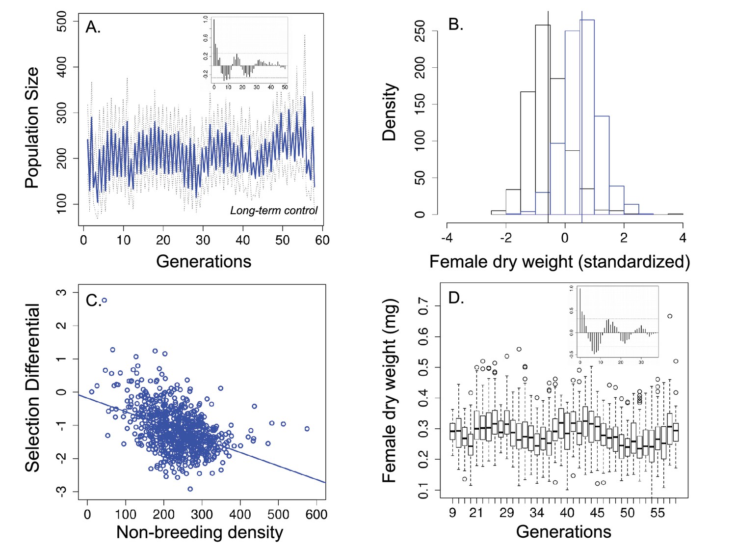
Population size, changes in body size and selection differentials for body size in the 'long-term control' experiment.
(a) Population size of seasonal flies cycled over 58 generations; (b) Female dry weight before (blue bars) and after (black bars) the non-breeding season. Vertical bars indicate the mean female dry weight before and after the non-breeding season; (c) Increased population size in the non-breeding season led to stronger directional selection for smaller flies. (d) Time series of female dry weight measured at the end of the non-breeding season over 38 generations. In (a and (d), the autocorrelograms (insets) showed evidence of cycles in both population size and body size. In (a solid blue line denotes mean population size for each generation from all replicates and dotted lines denote ±1 s.d. In (d, the horizontal line within each box represents the median value, the edges are 25th and 75th percentiles, the whiskers extend to the most extreme data points, and points are potential outliers.
Figure 3
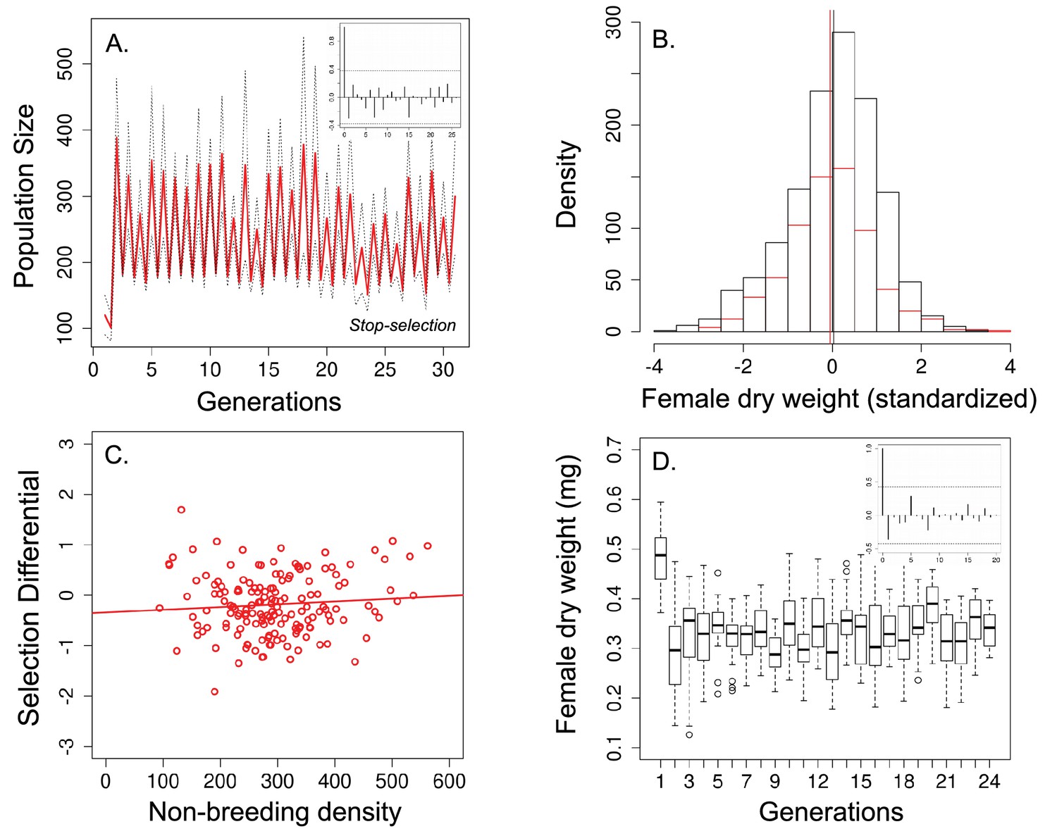
Population size, changes in body size and selection differential for body size in the 'stop-selection' experiment.
(a) Population size of seasonal flies cycled over 31 generations. Unlike the ‘long-term control, (b) there was no significant change in body size after the non-breeding season (female dry weight before - red bars - and after -black bars- the non-breeding season; vertical bars indicates the mean female dry weight before and after the non-breeding season) and (c) no evidence that selection for smaller flies was density dependence. (d) Time series of female dry weight measured at the end of the non-breeding season over 27 generations. In (a) and (d), the autocorrelograms (insets) showed no evidence of cycles in population or body size. In a solid red line denotes the mean population size for each generation from all replicates and dotted lines denote ±1 s.d. In (d), the horizontal line within each box represents the median value, the edges are 25th and 75th percentiles, the whiskers extend to the most extreme data points, and points are potential outliers.
Figure 4
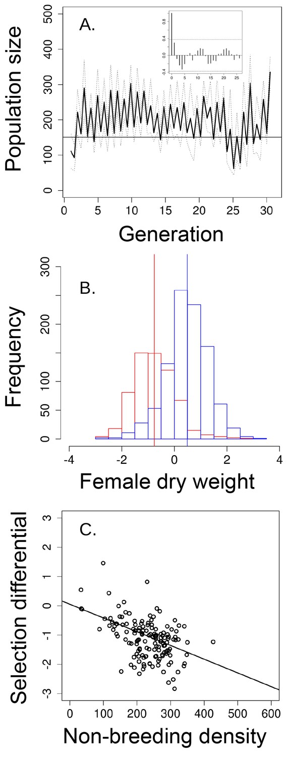
Population size, changes in body size and selection differentials for body size in the 'short-term control' experiment.
(a) Population size of seasonal flies cycled over 31 generations, as suggested by the autocorrelogram (insets), (b) female dry weight before the non-breeding season (blue bars) was higher than after the non-breeding season (red bars; vertical bars indicate the mean female dry weight before and after the non-breeding season). (c) increased population size in the non-breeding season led to stronger directional selection for smaller flies. In (a) solid black line denotes mean population size for each generation from all replicates and dotted lines denote ±1 s.d. In (d, the horizontal line within each box represents the median value, the edges are 25th and 75th percentiles, the whiskers extend to the most extreme data points, and points are potential outliers.
Figure 5
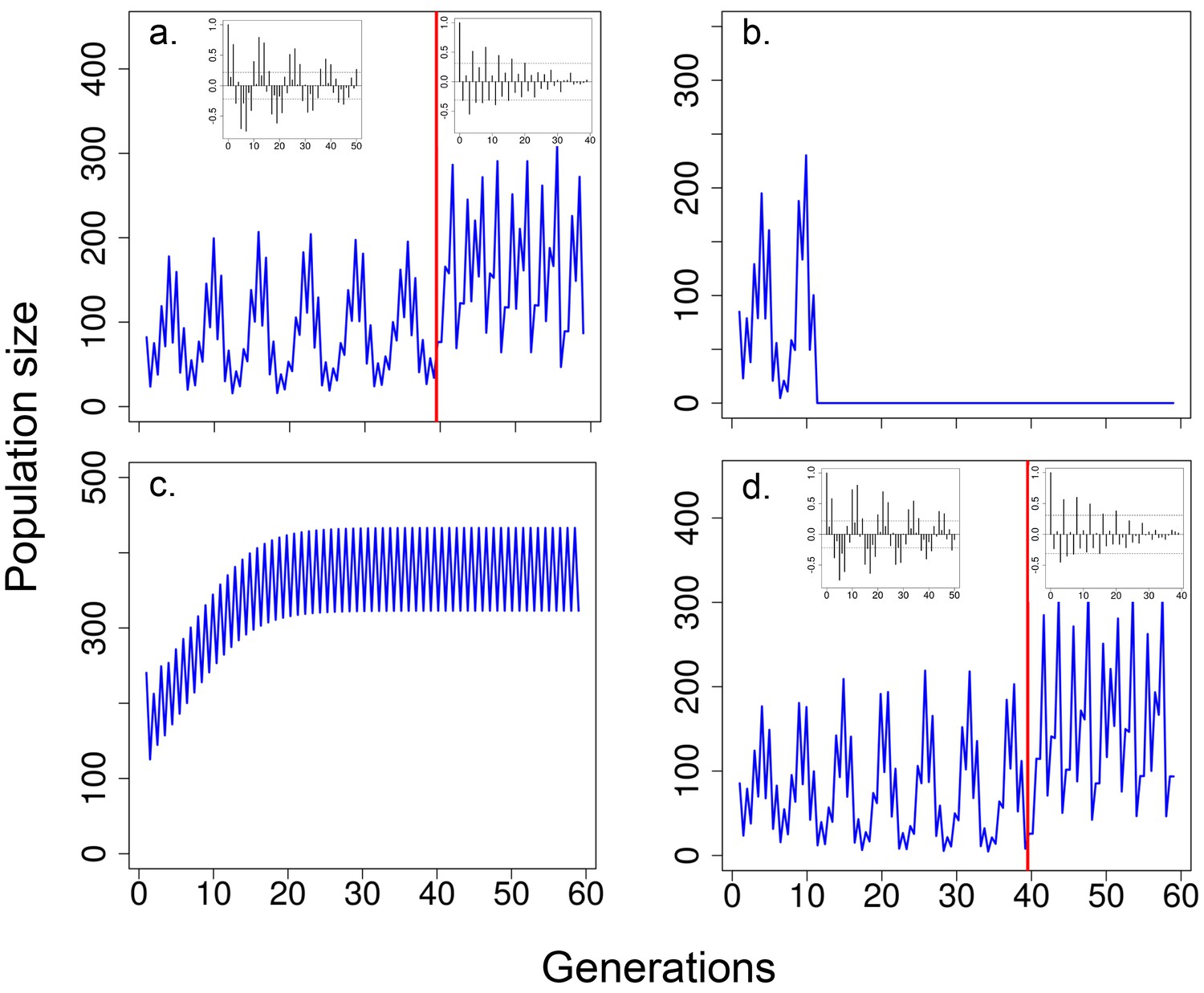
Predicted population size according to the integral projection model.
Time series generated with the model where, (a) for the first 40 generations (before vertical red line), when both viability selection and delayed density effects on survival during the non-breeding season and fecundity were operating and, for the last 20 generations, only the effects of current population size on fecundity and survival were modelled (i.e. no viability selection and no delayed density effects); (b) population size excluding the effects of viability selection (only the effects of delayed density dependence on fecundity and survival were operating) or (c) excluding the effects of delayed density dependence (only the effects of viability selection were operating). In (d), times series were generated as in (a) but with low heritability (see Results for details). In (b), population crashed (i.e. population size <1) at generation 10. In both (b) and (c), the model incorporated the effects of current abundance on fecundity and survival and heritability for body size. In (a) and (d) inset figures represent autocorrelograms for population size obtained from the mathematical model including delayed density dependence, viability and fecundity selection (before red line) or without both delayed density dependence and viability selection (after red line). See Material and methods for details and model parameters.
Figure 6
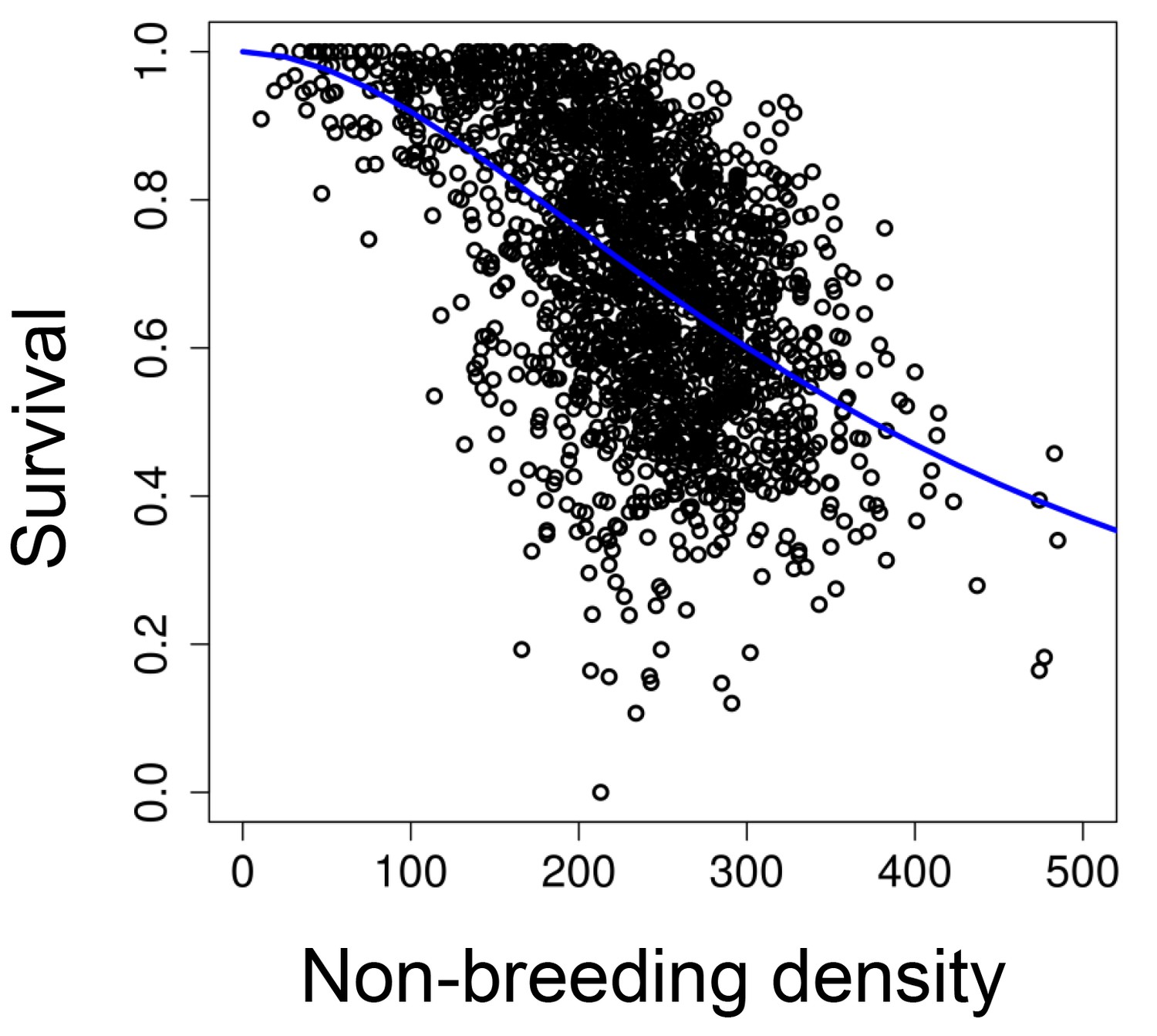
The relationship between survival and population size at the beginning of the non-breeding season.
The blue line represents a survival function parameterized with our 'long-term control' populations (v = 375.22, s.e.=7.60, t = 49.43, p<0.001; w = 1.83, s.e.=0.08, t = 22.50, p<0.001).
Appendix 1—figure 1
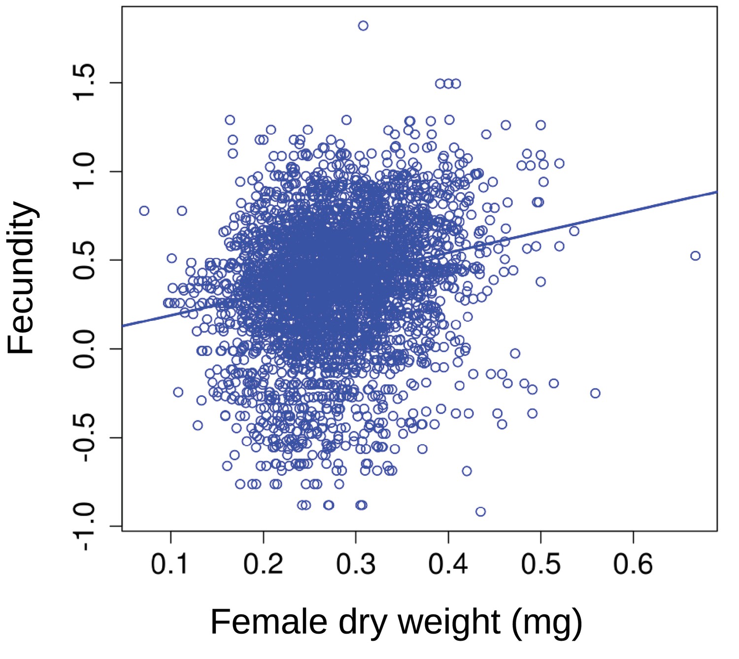
Fecundity as a function of average female dry weight at the beginning of the breeding season.
Larger individuals tend to have higher fecundity. The solid line represents the linear mixed effect model line for female dry weight (Appendix 1—table 1).
Appendix 2—figure 1
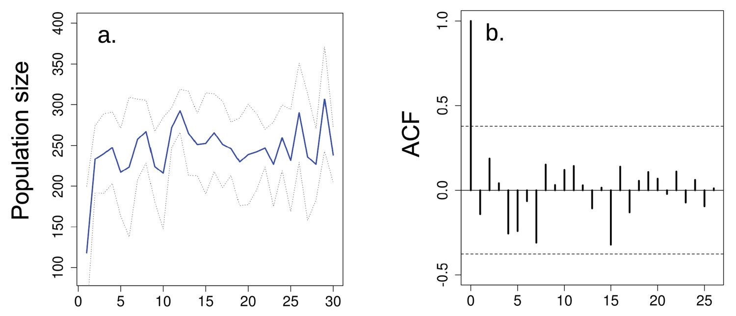
Overall effect of seasonality in multigenerational cycles.
(a) Population size of ‘aseasonal’ populations over 30 generations do not present evidence of multigenerational cycles according to the (b) autocorrelation plots. In a solid blue line denotes mean population size for each generation from all replicates and dotted lines denote ±1 s.d.
Appendix 3—figure 1
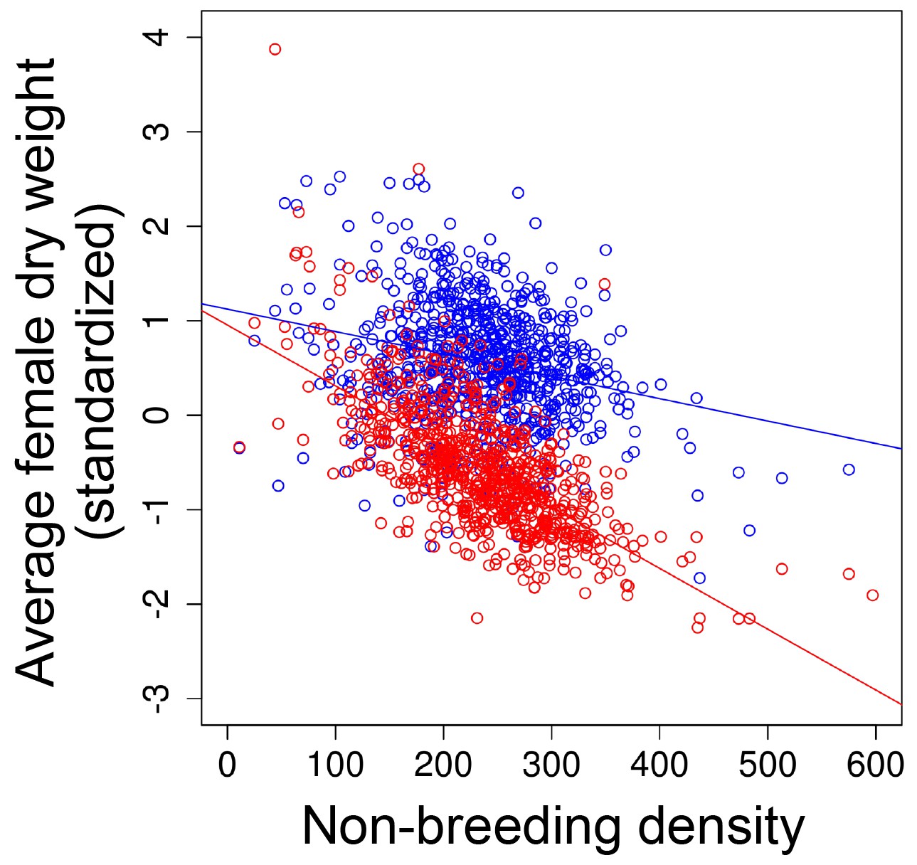
The strength of selection on body weight in seasonal environments.
As non-breeding density increased, the magnitude of directional selection for reduced dry weight also increased (Figure 2c in the main text). This relationship was driven by changes in the weight after (red points) rather than before (blue points) the non-breeding season. Solid lines indicate the linear mixed effect model line for non-breeding density before (blue line) and after (red line) the non-breeding season.
Author response image 1

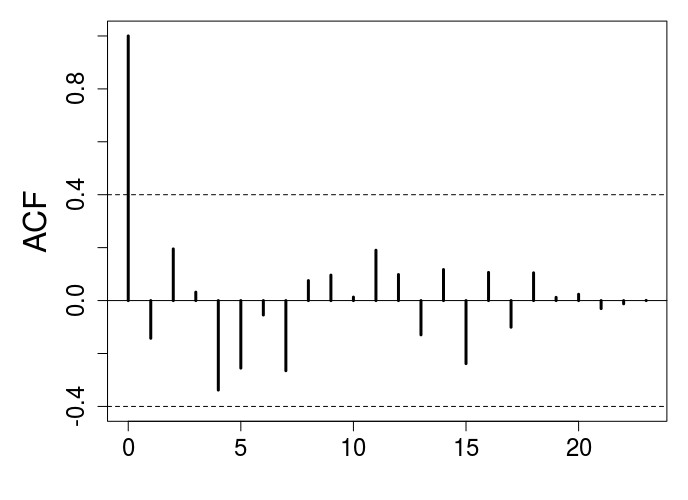
ACF plot for the long-term control after eliminating the first 6 generations to avoid transient dynamics.
Note that the peak at lag 16 crosses the confidence interval line.
Author response image 2
ACF plot for the stop-selection treatment after eliminating the first 6 generations to avoid transient dynamics.
There is no evidence of periodicity.
Tables
Table 1
Parameter estimates obtained from linear mixed effect models to investigate viability selection on body size as a function of thenumber of individuals at the beginning of the non-breeding season. In the ‘long-term control’, R2LMM(m)=0.18 and R2LMM(c)=0.20; in the 'stop selection' treatment, R2LMM(m)=0.006 and R2LMM(c)=0.006; and in the 'short-term control', R2LMM(m)=0.22 and R2LMM(c)=0.22. R2LMM(m) is the variance on the response variable that is explained only by the fixed effects and R2LMM(c) is the variance that is explained by both fixed and random effects. In all models, the selection differential was the response variable, abundance at the beginning of the non-breeding season was the fixed effect and population (vial) was the random effect.
Parameters | Fixed effects estimate | SE | Df | T | P |
|---|---|---|---|---|---|
1. Long-term control | |||||
Intercept | −0.181 | 0.081 | 434.5 | −2.22 | 0.027 |
Non-breeding abundance | −0.004 | 0.003 | 745.3 | −12.67 | <0.001 |
2. Stop selection | |||||
Intercept | −0.341 | 0.159 | 159 | −2.15 | 0.033 |
Non-breeding abundance | 0.001 | 0.001 | 159 | 1.06 | 0.291 |
3. Short-term control | |||||
Intercept | 0.028 | 0.184 | 100 | −0.15 | 0.880 |
Non-breeding abundance | −0.005 | 0.001 | 139 | −6.44 | <0.001 |
Table 2
Parameter estimates obtained from linear mixed effect models to investigate the effects of current and past density on fecundity in the ‘long-term control’, ‘stop-selection’ and ‘short-term control’ experiments. B refers to population size at the beginning of the breeding season in the current season and NB refers to population size at the beginning of the previous non-breeding season. In the ‘long-term control’, R2LMM(m)=0.34 and R2LMM(c)=0.37; in the 'stop selection' treatment, R2LMM(m)=0.07 and R2LMM(c)=0.07; and in the 'short-term control', R2LMM(m)=0.30 and R2LMM(c)=0.30.
Parameters | Fixed effects estimate | SE | T | P |
|---|---|---|---|---|
1. Long-term control | ||||
Intercept | 0.450 | 0.012 | 37.445 | <0.001 |
B | −0.212 | 0.008 | −25.82 | <0.001 |
NB | −0.008 | 0.008 | −1.05 | 0.296 |
B * NB | 0.026 | 0.005 | 5.07 | <0.001 |
2. Stop-selection | ||||
Intercept | 0.551 | 0.024 | 22.91 | <0.001 |
B | 0.150 | 0.053 | 2.82 | 0.005 |
NB | −0.156 | 0.034 | −4.53 | <0.001 |
B * NB | 0.0613 | 0.03 | 2.31 | 0.021 |
2. Short-term control | ||||
Intercept | 0.532 | 0.019 | 27.72 | <0.001 |
B | −0.226 | 0.024 | −9.34 | <0.001 |
NB | −0.039 | 0.022 | −1.74 | 0.083 |
B * NB | 0.046 | 0.017 | 2.65 | 0.008 |
Table 3
Parameter estimates obtained from linear mixed effect models to investigate the effects of current and past density on survival in the ‘long-term control’, ‘stop-selection’ and ‘short-term control’ experiments. NB refers to population size at the beginning of the non-breeding season in the current generation. B1, NB1, B2 and NB2, refers the population size at the beginning of each season going back 1 or two generations, respectively. In the ‘long-term control’, R2LMM(m)=0.35 and R2LMM(c)=0.36; in the 'stop selection' treatment, R2LMM(m)=0.99 and R2LMM(c)=0.99; and in the 'short-term control', R2LMM(m)=0.43 and R2LMM(c)=0.43.
Parameters | Fixed effects estimate | SE | T | P |
|---|---|---|---|---|
1. Long-term control | ||||
Intercept | −0.353 | 0.006 | −54.74 | <0.001 |
NB | −0.186 | 0.006 | −31.19 | <0.001 |
B1 | 0.106 | 0.008 | 13.76 | <0.001 |
NB1 | −0.056 | 0.007 | −8.34 | <0.001 |
B2 | 0.044 | 0.007 | 5.67 | <0.001 |
NB2 | −0.020 | 0.007 | −2.89 | 0.004 |
2. Stop-selection | ||||
Intercept | −0.489 | 0.001 | −1,068.62 | <0.001 |
NB | −0.213 | 0.001 | −412.71 | <0.001 |
B1 | 0.001 | 0.001 | 1.325 | 0.186 |
NB1 | −0.001 | 0.001 | −1.235 | 0.217 |
B2 | 0.001 | 0.001 | 0.479 | 0.632 |
NB2 | 0.001 | 0.001 | 0.225 | 0.822 |
3. Short-term control | ||||
Intercept | −0.427 | 0.013 | −33.36 | <0.001 |
NB | −0.223 | 0.0142 | −15.64 | <0.001 |
B1 | 0.144 | 0.015 | 7.22 | <0.001 |
NB1 | −0.037 | 0.015 | −2.40 | 0.017 |
B2 | 0.041 | 0.020 | 2.03 | 0.043 |
NB2 | −0.015 | 0.016 | −0.933 | 0.351 |
Appendix 1—table 1
Parameter estimates obtained from a linear mixed effect model with fecundity as a response variable and average female dry weight at the beginning of the breeding season as explanatory variable. R2LMM(m)=0.04 and R2LMM(c)=0.14.
| Parameters | SE | df | t | p | |
|---|---|---|---|---|---|
Fixed effects estimate | |||||
Intercept | 0.072 | 0.043 | 260 | 1.69 | 0.101 |
Female dry weight | 1.178 | 0.092 | 3601 | 12.82 | <0.001 |
Random effect variance | |||||
Population | 0.015 | ||||
Residual | 0.125 |
Appendix 3—table 1
Parameter estimates obtained from a linear mixed effect models to investigate variation in female dry weight as a function of the interaction between density at the beginning of the non-breeding season and whether weight was measured before or after the non-breeding season. Status refers to a dummy variable indicating the time when body size was measured (before or after the non-breeding season). Reference value was after the non-breeding season. Marginal (only taking account the fixed effects) and conditional (taking into account both fixed and random effects) coefficient of determination were R2LMM(m)=0.42 and R2LMM(c)=0.50, respectively. In all models, population and generation were entered as random effects.
| Parameters | SE | dfDf | tT | pP | |
|---|---|---|---|---|---|
Fixed effects estimate | |||||
Intercept | 0.680 | 0.06 | 266 | 10.31 | <0.001 |
Non-breeding density | 0.005 | 0.0002 | 900 | −29.38 | <0.001 |
Status Before | 0.430 | 0.009 | 896 | 7.55 | <0.001 |
Non-breeding density:Status | 0.003 | 0.0001 | 892 | 14.11 | <0.001 |
Random effect variance | SD | ||||
Generation | 0.045 | 0.212 | |||
Population | 0.037 | 0.193 | |||
Residual | 0.474 | 0.688 |
Download links
A two-part list of links to download the article, or parts of the article, in various formats.
Downloads (link to download the article as PDF)
Open citations (links to open the citations from this article in various online reference manager services)
Cite this article (links to download the citations from this article in formats compatible with various reference manager tools)
A fitness trade-off between seasons causes multigenerational cycles in phenotype and population size
eLife 6:e18770.
https://doi.org/10.7554/eLife.18770


