Figures and data in Structure in the variability of the basic reproductive number (R0) for Zika epidemics in the Pacific islands

Figures
Tables
Additional files

21 figures, 7 tables and 5 additional files

Figures

Figure 1

Download asset Open asset

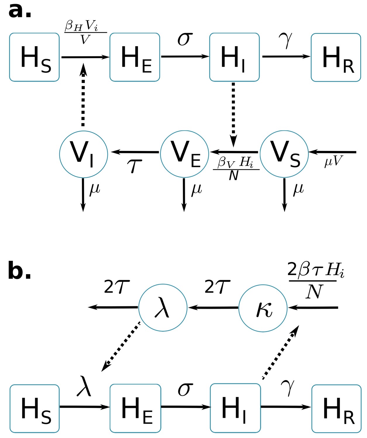
Graphical representation of compartmental models.

Squared boxes and circles correspond respectively to human and vector compartments. Plain arrows represent transitions from one state to the next. Dashed arrows indicate interactions between humans and vectors. (a) Pandey model (Pandey et al., 2013). $H_{S}$ susceptible individuals; $H_{E}$ infected (not yet infectious) individuals; $H_{I}$ infectious individuals; $H_{R}$ recovered individuals; $σ$ is the rate at which $H_{E}$ -individuals move to infectious class $H_{I}$ ; infectious individuals ( $H_{I}$ ) then recover at rate $γ$ ; $V_{S}$ susceptible vectors; $V_{E}$ infected (not yet infectious) vectors; $V_{I}$ infectious vectors; $V$ constant size of total mosquito population; $τ$ is the rate at which $V_{E}$ -vectors move to infectious class $V_{I}$ ; vectors die at rate $μ$ . (b) Laneri model (Laneri et al., 2010). $H_{S}$ susceptible individuals; $H_{E}$ infected (not yet infectious) individuals; $H_{I}$ infectious individuals; $H_{R}$ recovered individuals; $σ$ is the rate at which $H_{E}$ -individuals move to infectious class $H_{I}$ ; infectious individuals ( $H_{I}$ ) then recover at rate $γ$ ; implicit vector-borne transmission is modeled with the compartments $κ$ and $λ$ ; $λ$ current force of infection; $κ$ latent force of infection reflecting the exposed state for mosquitoes during the extrinsic incubation period; $τ$ is the transition rate associated to the extrinsic incubation period.

https://doi.org/10.7554/eLife.19874.003

Figure 2

Download asset Open asset

Results using the Pandey model.

Posterior median number of observed Zika cases (solid line), 95% credible intervals (shaded blue area) and data points (black dots). First column: particle filter fit. Second column: Simulations from the posterior density. Third column: $R_{0}$ posterior distribution. (a) Yap. (b) Moorea. (c) Tahiti. (d) New Caledonia. The estimated seroprevalences at the end of the epidemic (with 95% credibility intervals) are: (a) 73% (CI95: 68–77, observed 73%); (b) 49% (CI95: 45–53, observed 49%); (c) 49% (CI95: 45–53, observed 49%); (d) 39% (CI95: 8–92). See Figure 4.

https://doi.org/10.7554/eLife.19874.004

Figure 3

Download asset Open asset

Results using the Laneri model.

Posterior median number of observed Zika cases (solid line), 95% credible intervals (shaded blue area) and data points (black dots). First column: particle filter fit. Second column: Simulations from the posterior density. Third column: $R_{0}$ posterior distribution. (a) Yap. (b) Moorea. (c) Tahiti. (d) New Caledonia. The estimated seroprevalences at the end of the epidemic (with 95% credibility intervals) are: (a) 72% (CI95: 68–77, observed 73%); (b) 49% (CI95: 45–53, observed 49%); c) 49% (CI95: 45–53, observed 49%); d) 65% (CI95: 24–91). See Figure 5.

https://doi.org/10.7554/eLife.19874.005

Figure 4

Download asset Open asset

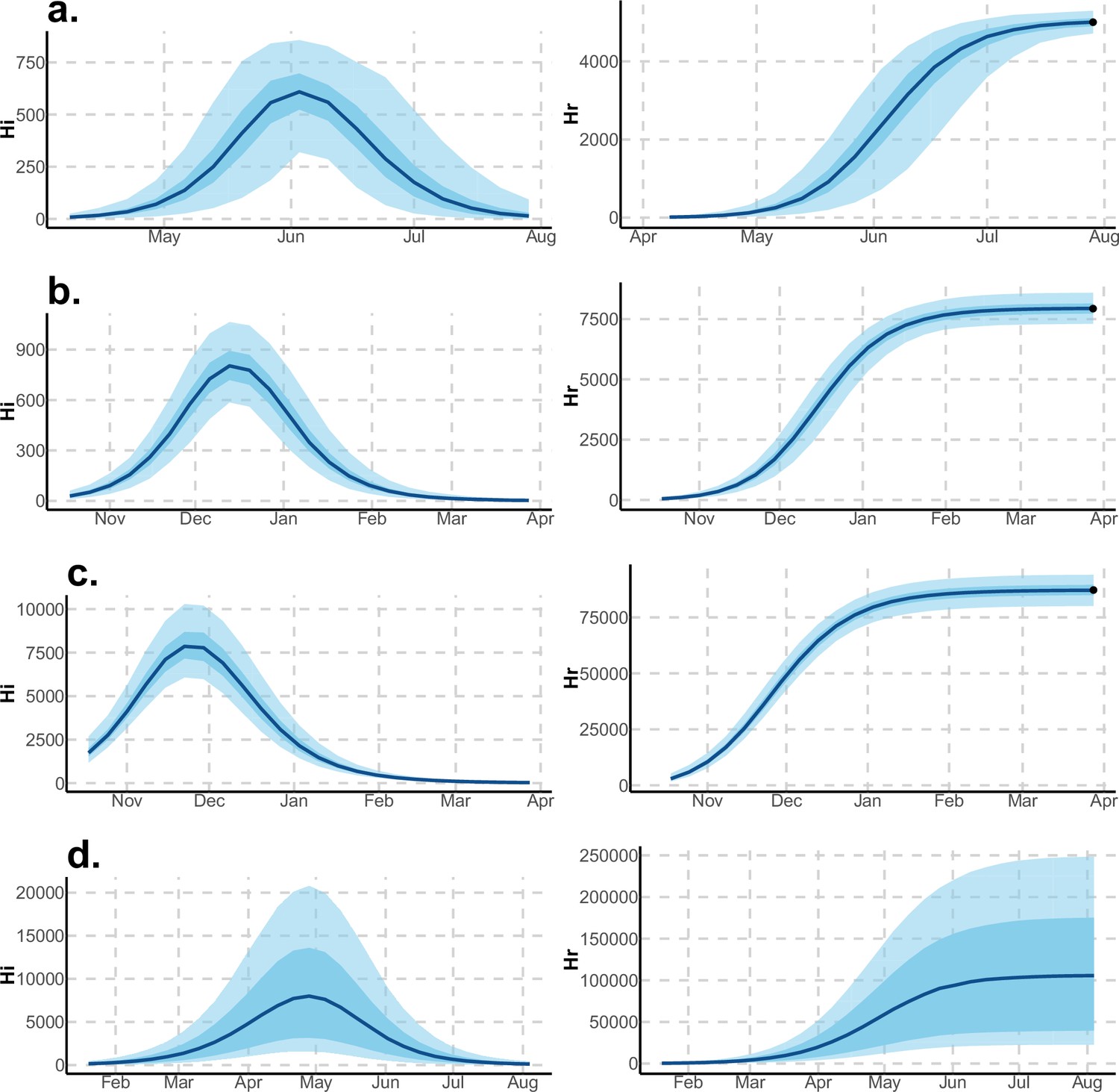
Infected and recovered humans evolution during the outbreak with Pandey model.

Simulations from the posterior density: posterior median (solid line), 95% and 50% credible intervals (shaded blue areas) and observed seroprevalence (black dots). First column: Infected humans ( $H_{I}$ ). Second column: Recovered humans ( $H_{R}$ ). (a) Yap. (b) Moorea. (c) Tahiti. (d) New Caledonia.

https://doi.org/10.7554/eLife.19874.013

Figure 5

Download asset Open asset

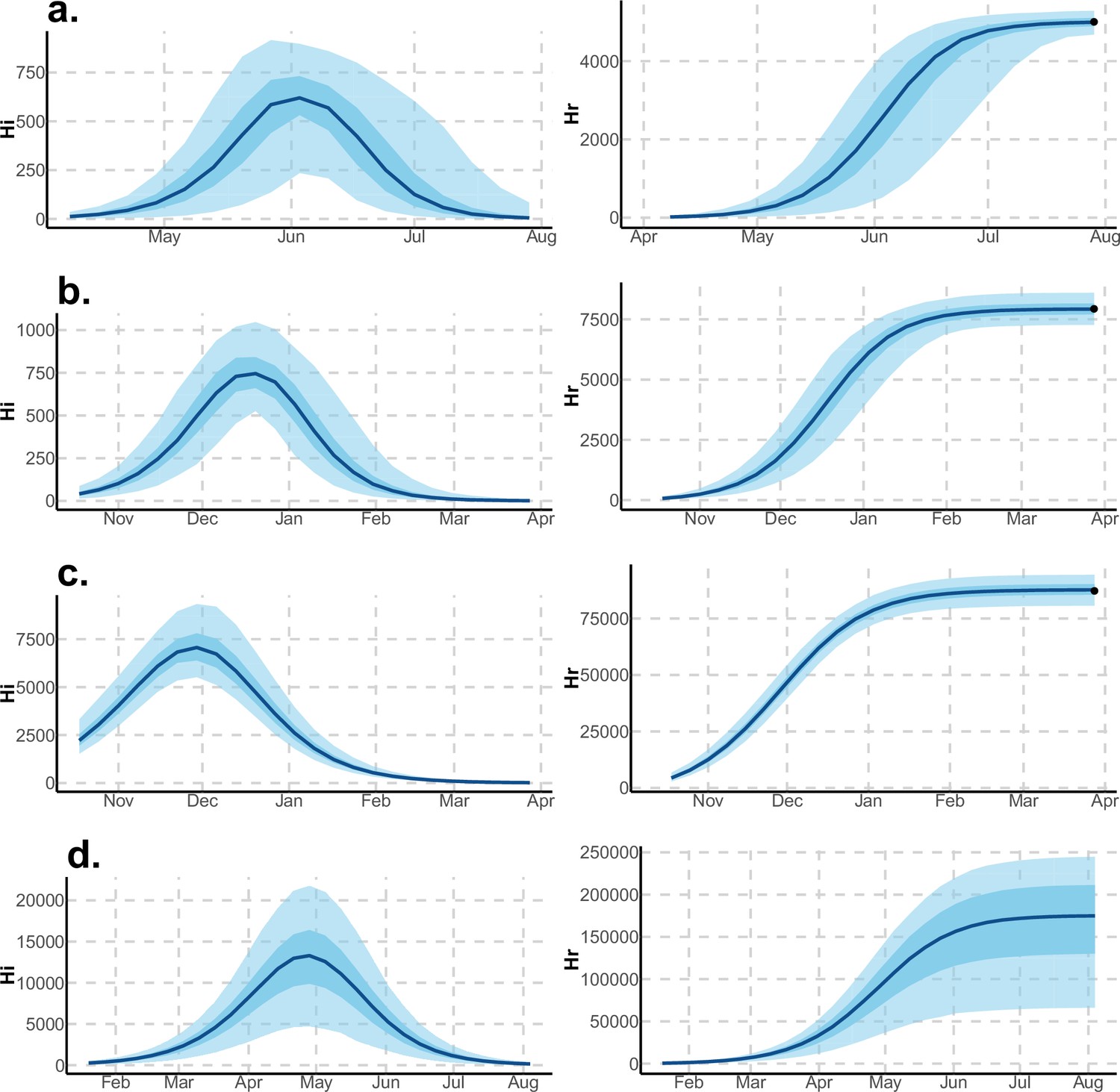
Infected and recovered humans evolution during the outbreak with Laneri model.

Simulations from the posterior density: posterior median (solid line), 95% and 50% credible intervals (shaded blue areas) and observed seroprevalence (black dots). First column: Infected humans ( $H_{I}$ ). Second column: Recovered humans ( $H_{R}$ ). (a) Yap. (b) Moorea. (c) Tahiti. (d) New Caledonia.

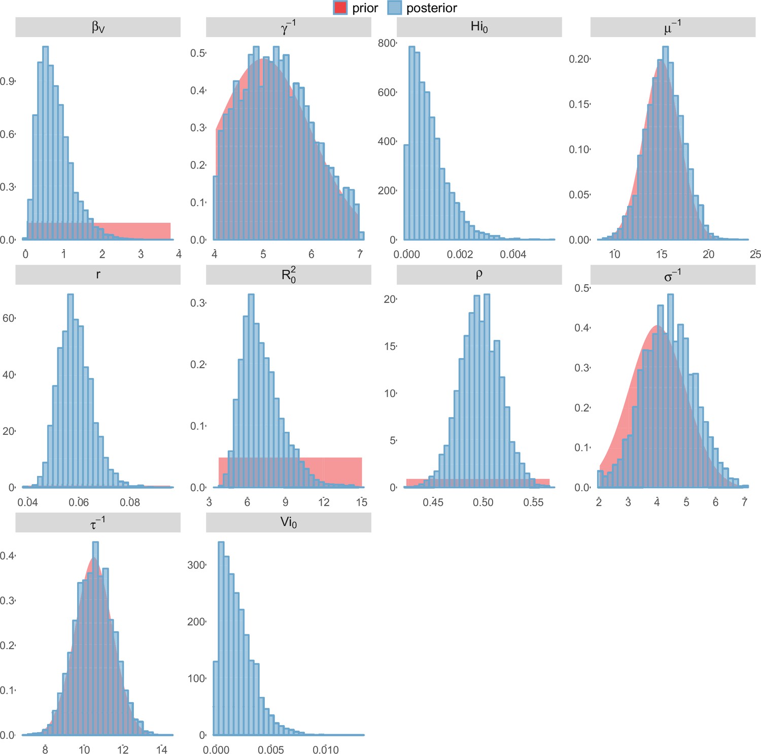
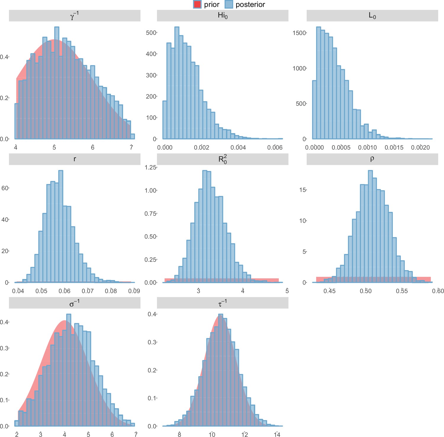
https://doi.org/10.7554/eLife.19874.014

Figure 6

Download asset Open asset

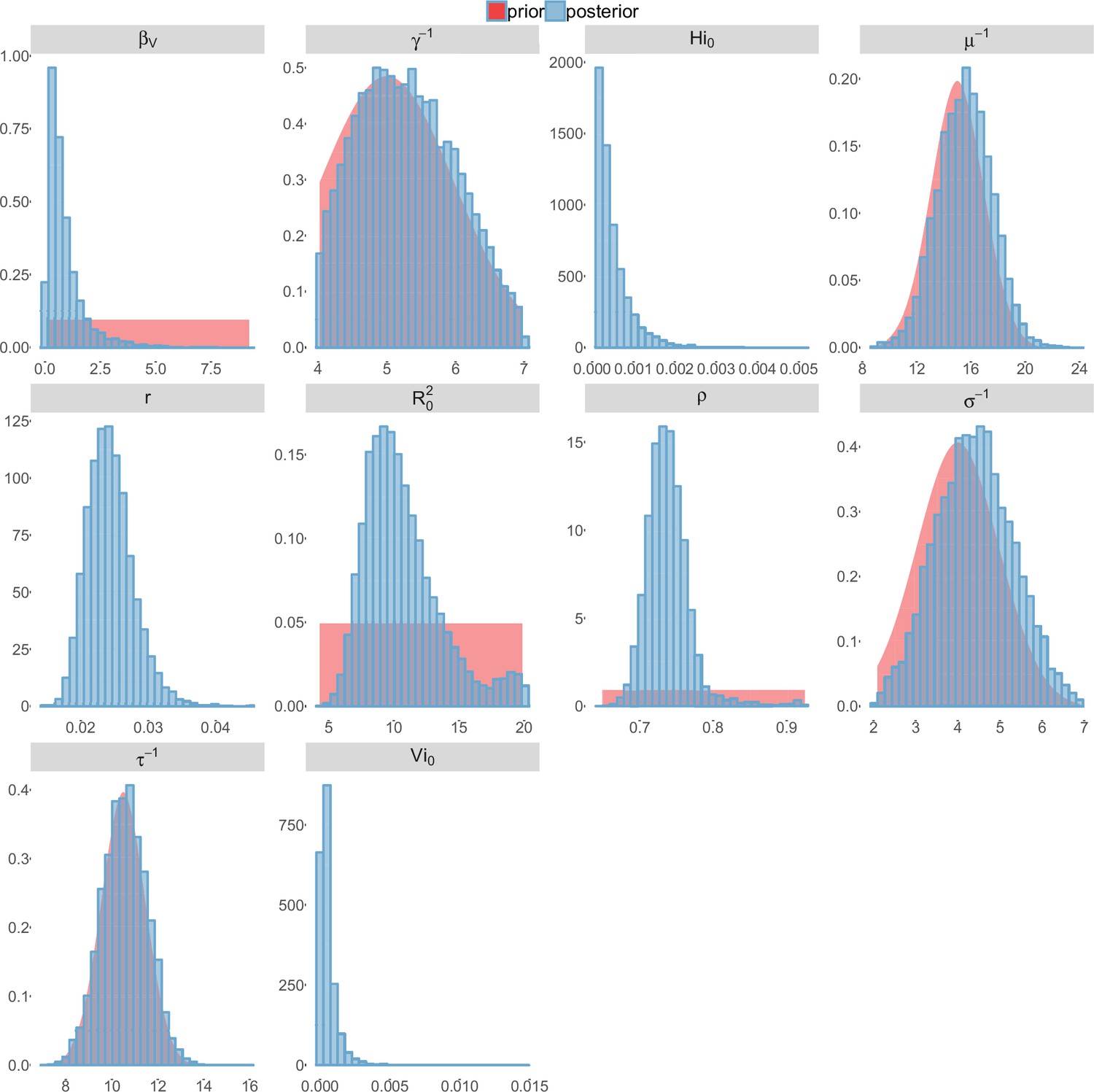
Posterior distributions.

Pandey model, Yap island.

https://doi.org/10.7554/eLife.19874.015

Figure 7

Download asset Open asset

Posterior distributions.

Pandey model, Moorea island.

https://doi.org/10.7554/eLife.19874.016

Figure 8

Download asset Open asset

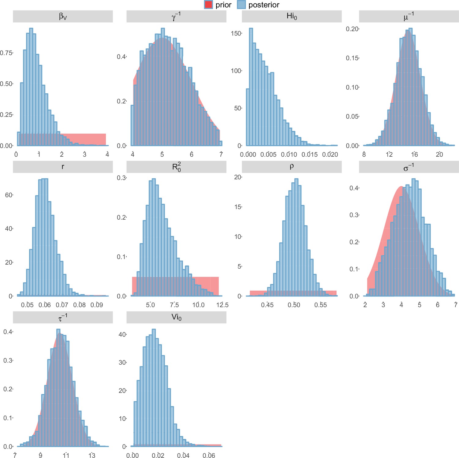
Posterior distributions.

Pandey model, Tahiti island.

https://doi.org/10.7554/eLife.19874.017

Figure 9

Download asset Open asset

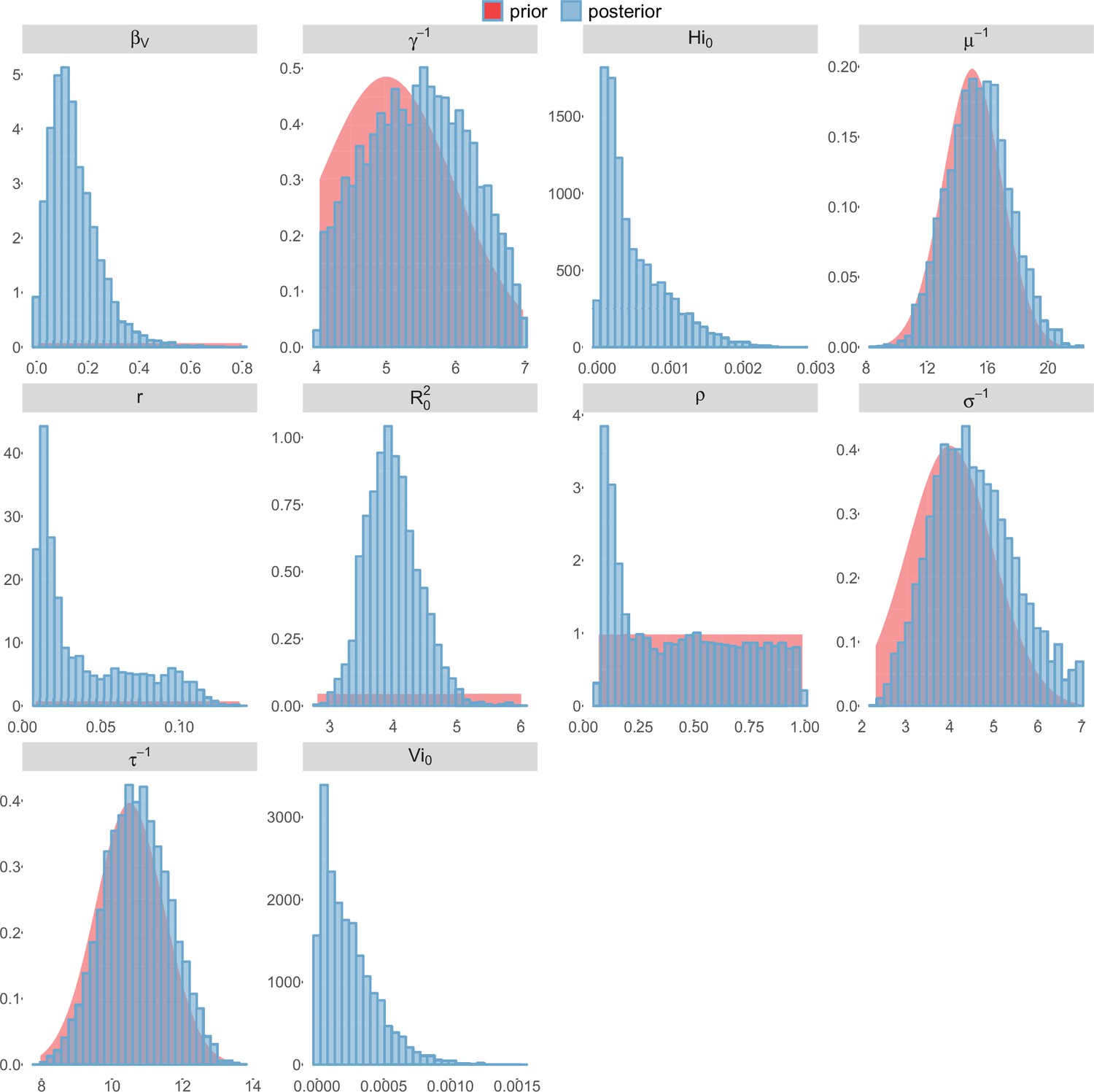
Posterior distributions.

Pandey model, New Caledonia.

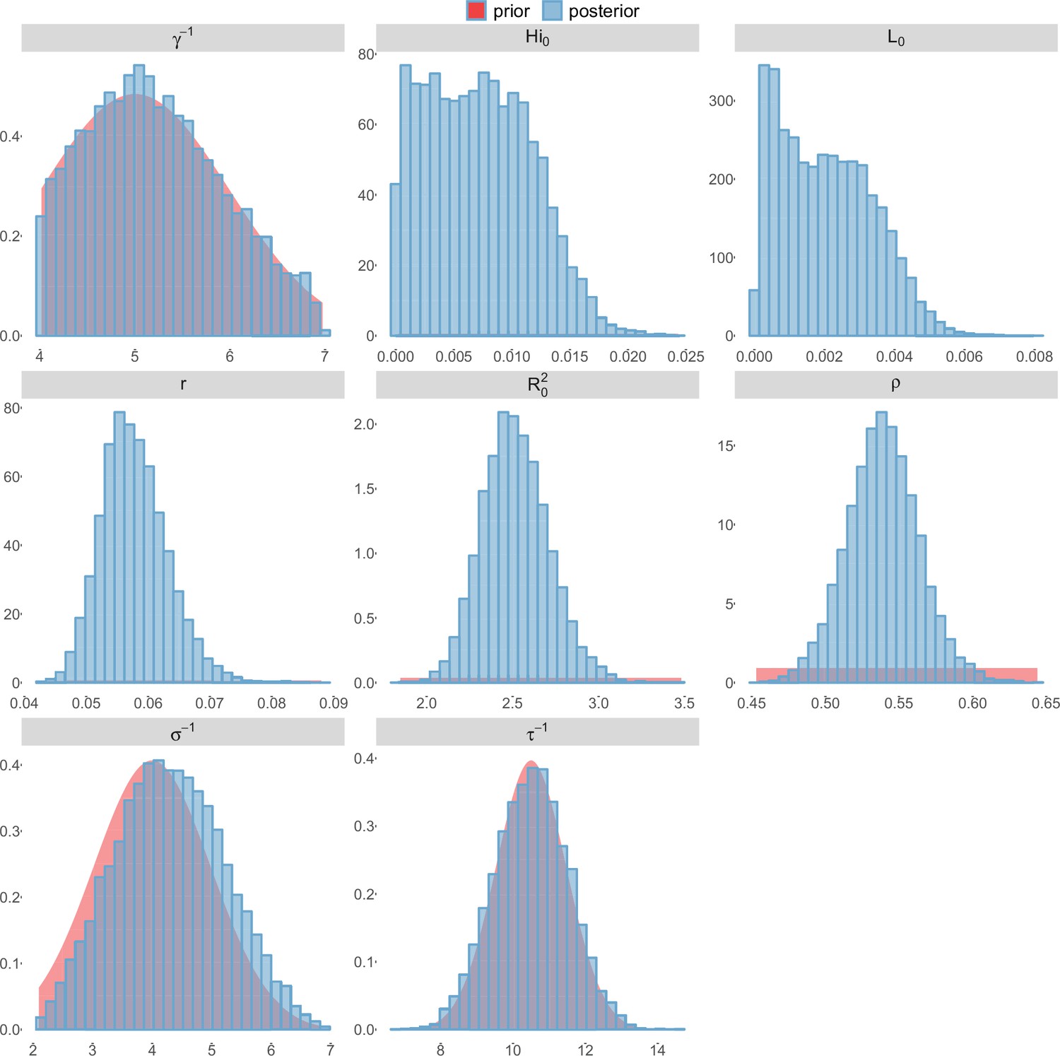
https://doi.org/10.7554/eLife.19874.018

Figure 10

Download asset Open asset

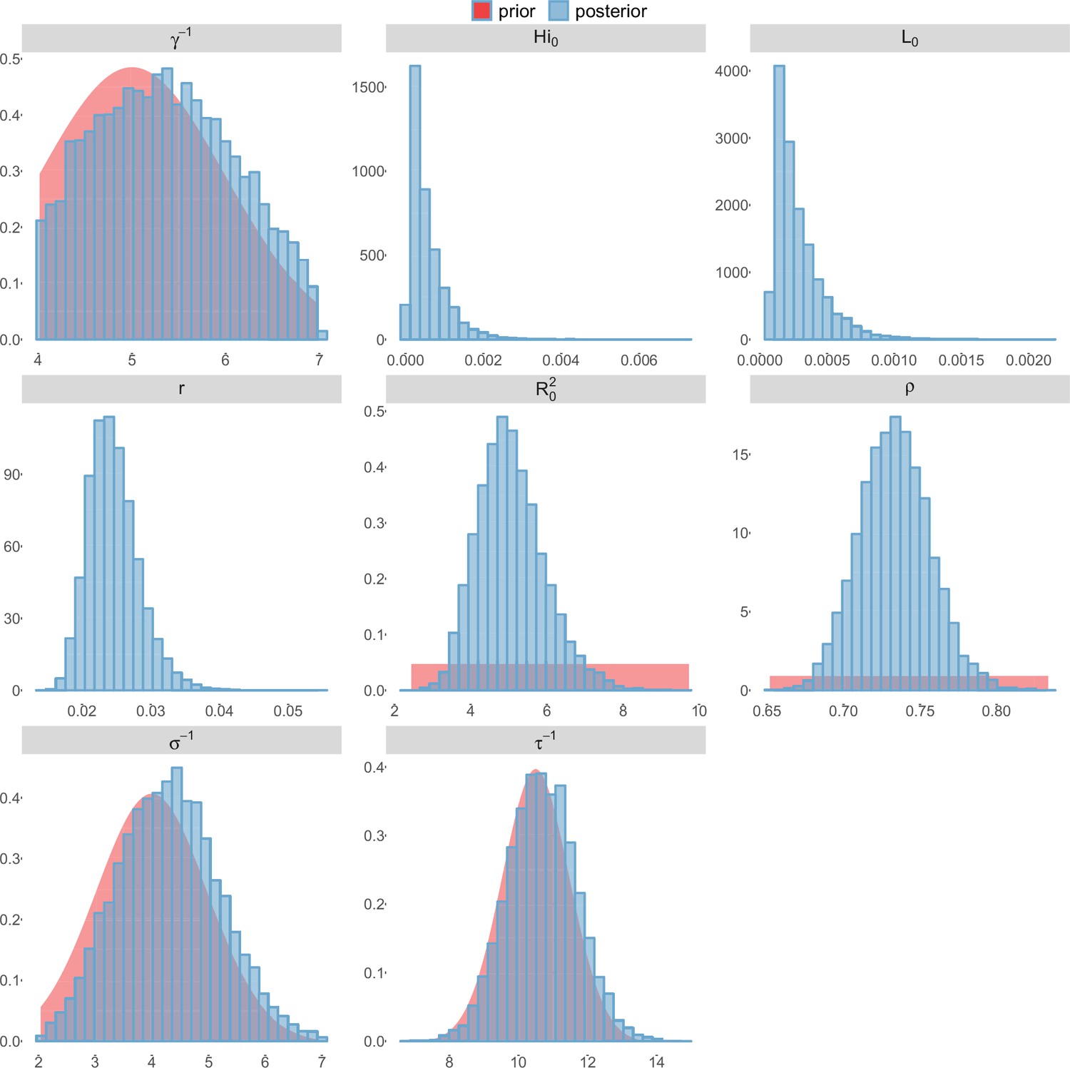
Posterior distributions.

Laneri model, Yap island.

https://doi.org/10.7554/eLife.19874.019

Figure 11

Download asset Open asset

Posterior distributions.

Laneri model, Moorea island.

https://doi.org/10.7554/eLife.19874.020

Figure 12

Download asset Open asset

Posterior distributions.

Laneri model, Tahiti island.

https://doi.org/10.7554/eLife.19874.021

Figure 13

Download asset Open asset

Posterior distributions.

Laneri model, New Caledonia.

https://doi.org/10.7554/eLife.19874.022

Figure 14

Download asset Open asset

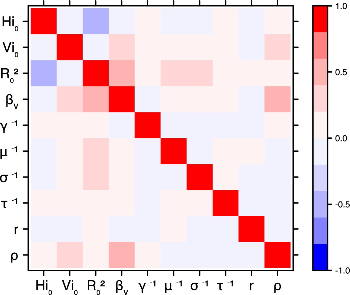
Correlation plot of MCMC output.

Pandey model, Yap island.

https://doi.org/10.7554/eLife.19874.023

Figure 15

Download asset Open asset

Correlation plot of MCMC output.

Pandey model, Moorea island.

https://doi.org/10.7554/eLife.19874.024

Figure 16

Download asset Open asset

Correlation plot of MCMC output.

Pandey model, Tahiti island.

https://doi.org/10.7554/eLife.19874.025

Figure 17

Download asset Open asset

Correlation plot of MCMC output.

Pandey model, New Caledonia.

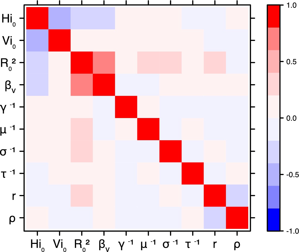
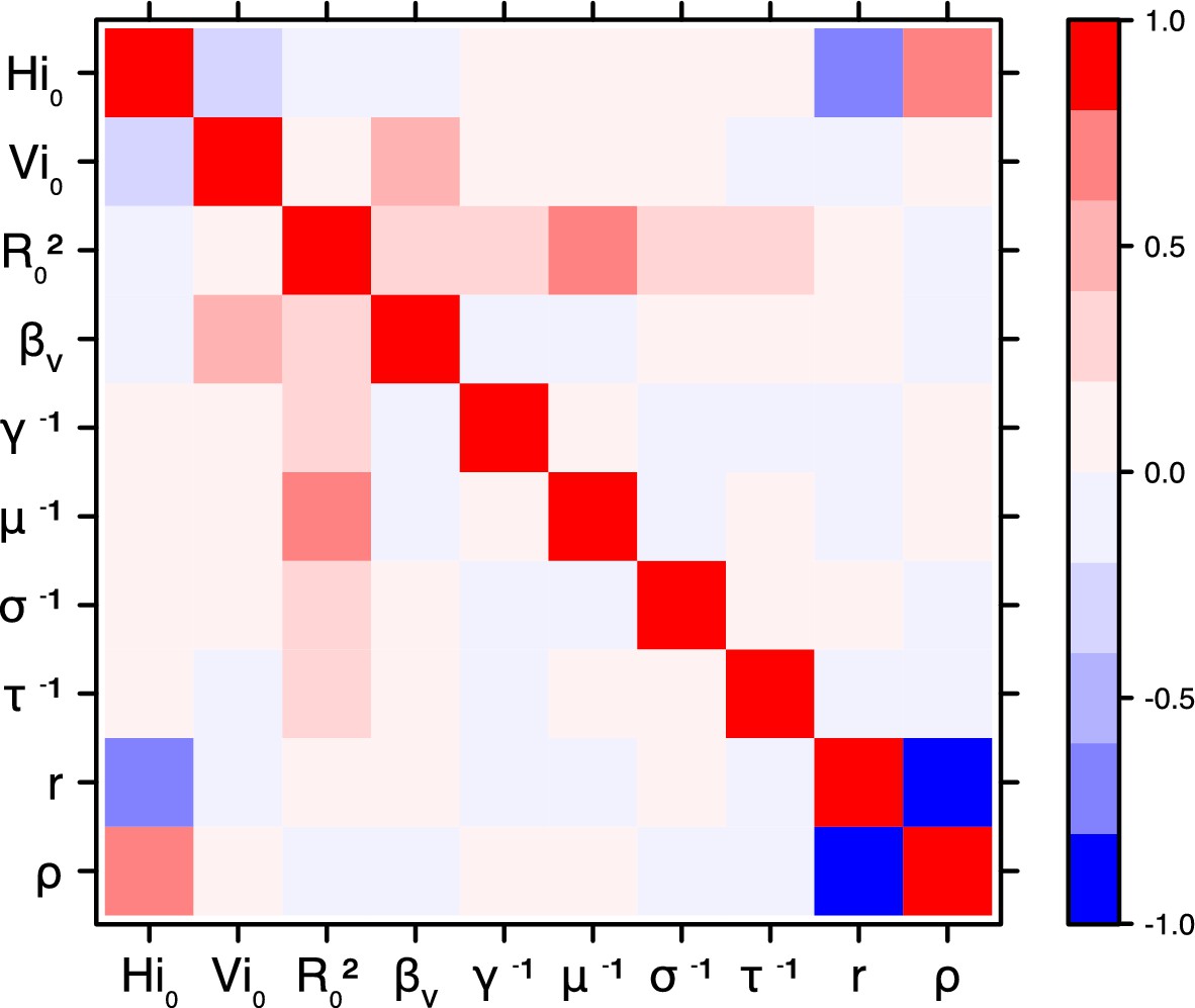
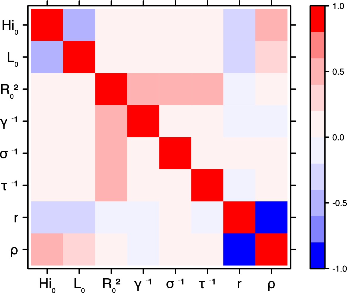
https://doi.org/10.7554/eLife.19874.026

Figure 18

Download asset Open asset

Correlation plot of MCMC output.

Laneri model, Yap island.

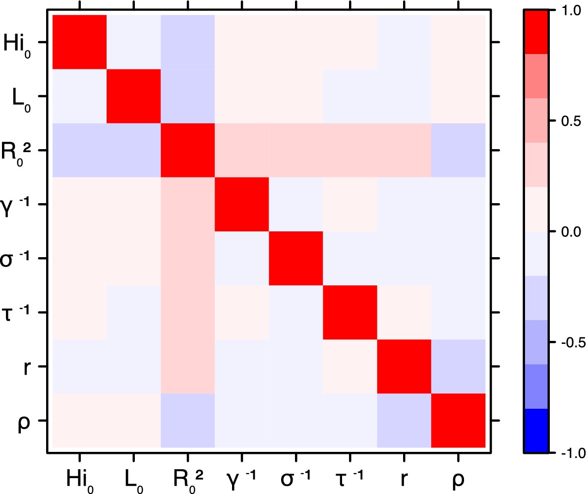
https://doi.org/10.7554/eLife.19874.027

Figure 19

Download asset Open asset

Correlation plot of MCMC output.

Laneri model, Moorea island.

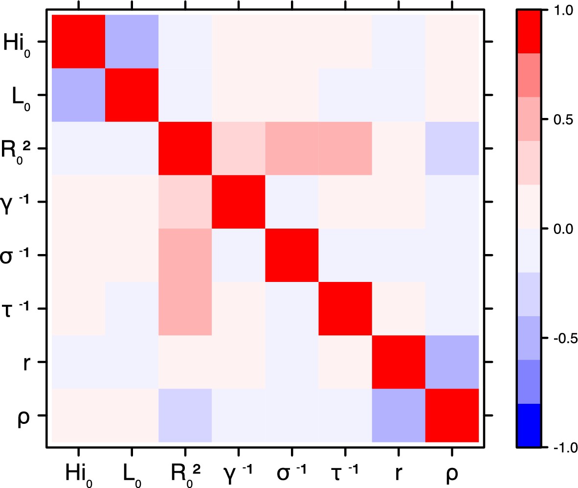
https://doi.org/10.7554/eLife.19874.028

Figure 20

Download asset Open asset

Correlation plot of MCMC output.

Laneri model, Tahiti island.

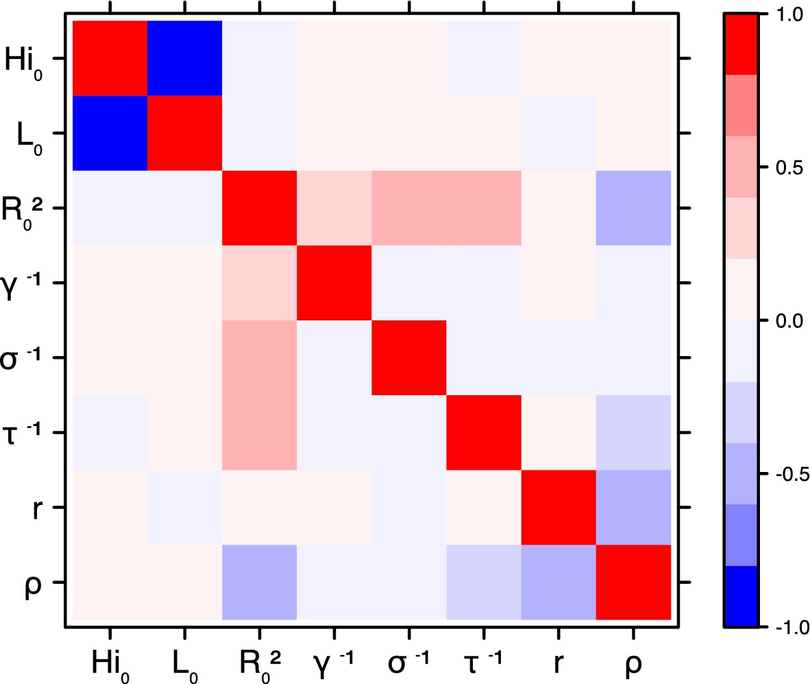
https://doi.org/10.7554/eLife.19874.029

Figure 21

Download asset Open asset

Correlation plot of MCMC output.

Laneri model, New Caledonia.

https://doi.org/10.7554/eLife.19874.030

Tables

Table 1

Parameter estimations for the Pandey model. Posterior median (95% credible intervals). All the posterior parameter distributions are presented in Figures 6–9 .

https://doi.org/10.7554/eLife.19874.006

Pandey model		Yap	Moorea	Tahiti	New Caledonia
Population size	H	6892	16,200	178,100	268,767
Basic reproduction number	$R_{0}$	3.2 (2.4–4.1)	2.6 (2.2–3.3)	2.4 (2.0–3.2)	2.0 (1.8–2.2)
Observation rate	$r$	0.024 (0.019-0.032)	0.058 (0.048-0.073)	0.060 (0.050-0.073)	0.024 (0.010-0.111)
Fraction of population involved	$ρ$	74% (69–81)	50% (48–54)	50% (46–54)	40% (9–96)
Initial number of infected individuals	$H_{I} (0)$	2 (1–8)	5 (0–21)	329 (16–1047)	37 (1–386)
Infectious period in human (days)	$γ^{- 1}$	5.2 (4.1–6.7)	5.2 (4.1–6.8)	5.2 (4.1–6.7)	5.5 (4.2–6.8)
Extrinsic incubation period in mosquito (days)	$τ^{- 1}$	10.6 (8.7–12.5)	10.5 (8.6–12.4)	10.5 (8.6–12.6)	10.7 (8.9–12.5)
Mosquito lifespan (days)	$μ^{- 1}$	15.6 (11.7–19.3)	15.3 (11.4–19.1)	15.1 (11.2–19.0)	15.4 (11.6–19.4)

Table 2

Parameter estimations for the Laneri model. Posterior median (95% credible intervals). All the posterior parameter distributions are presented in Figures 10–13.

https://doi.org/10.7554/eLife.19874.007

Laneri model		Yap	Moorea	Tahiti	New Caledonia
Population size	H	6892	16,200	178,100	268,767
Basic reproduction number	$R_{0}$	2.2 (1.9–2.6)	1.8 (1.6–2.0)	1.6 (1.5–1.7)	1.6 (1.5–1.7)
Observation rate	$r$	0.024 (0.019–0.033)	0.057 (0.047–0.07)	0.057 (0.049–0.069)	0.014 (0.010–0.037)
Fraction of population involved	$ρ$	73% (69–78)	51% (47–55)	54% (49–59)	71% (27–98)
Initial number of infected individuals	$H_{I} (0)$	2 (1–10)	9 (1–28)	667 (22–1570)	82 (2–336)
Infectious period in human (days)	$γ^{- 1}$	5.3 (4.1–6.6)	5.3 (4.1–6.7)	5.2 (4.1–6.7)	5.4 (4.1–6.8)
Extrinsic incubation period in mosquito (days)	$τ^{- 1}$	10.7 (8.8–12.7)	10.6 (8.6–12.6)	10.5 (8.5–12.5)	10.8 (8.9–12.8)

Table 3

Details of the observation models for seroprevalence

https://doi.org/10.7554/eLife.19874.008

Island	Date	Standard deviation	Observed seroprevalence
		$Λ$	$H_{R}^{o b s}$
Yap	2007-07-29	150	5005 (Duffy et al., 2009)
Moorea	2014-03-28	325	0.49 × 16200 = 7938 (Aubry et al., 2015b)
Tahiti	2014-03-28	3562	0.49 × 178100 = 87269 (Aubry et al., 2015b)

Table 4

Prior distributions of parameters. 'Uniform[0,20]' indicates a uniform distribution in the range [0,20]. 'Normal(5,1) in [4,7]' indicates a normal distribution with mean five and standard deviation 1, restricted to the range [4,7].

https://doi.org/10.7554/eLife.19874.009

Parameters		Pandey model	Laneri model	References
$R_{0}^{2}$	squared basic reproduction number	Uniform[0, 20]	Uniform[0, 20]	assumed
$β_{V}$	transmission from human to mosquito	Uniform[0,10]	.	assumed
$γ^{- 1}$	infectious period (days)	Normal(5,1) in [4,7]	Normal(5,1) in [4,7]	(Mallet et al., 2015)
$σ^{- 1}$	intrinsic incubation period (days)	Normal(4,1) in [2,7]	Normal(4,1) in [2,7]	(Nishiura et al., 2016b; Bearcroft, 1956; Lessler et al., 2016)
$τ^{- 1}$	extrinsic incubation period (days)	Normal(10.5,1) in [4,20]	Normal(10.5,1) in [4,20]	(Hayes, 2009; Chouin-Carneiro et al., 2016)
$μ^{- 1}$	mosquito lifespan (days)	Normal(15,2) in [4,30]	.	(Brady et al., 2013; Liu-Helmersson et al., 2014)
$ρ$	fraction of population involved	Uniform[0,1]	Uniform[0,1]

Initial conditions (t=0)		Pandey model	Laneri model
H_I(0)	infected humans	Uniform[10^-6,1]N	Uniform[10^-6,1]N
H_E(0)	exposed humans	H_I(0)	H_I(0)
H_R(0)	recovered humans	0	0
	infected vectors	V_I(0)=Uniform[10^-6,1]H	L(0)=Uniform[10^-6,1]N
	exposed vectors	V_E(0) = V_I(0)	K(0)=L(0)

Local conditions		Yap	Moorea	Tahiti	New Caledonia	References
r	observation rate	Uniform[0,1]	Uniform[0,1]	Uniform[0,0.3]	Uniform[0,0.23]	(Mallet et al., 2015; DASS, 2014)
H	population size	6,892	16,200	178,100	268,767	(Duffy et al., 2009; Insee, 2012, 2014)

Table 5

Square root of the number of secondary cases after the introduction of a single infected individual in a naive population. Median and 95% credible intervals of 1000 deterministic simulations using parameters from the posterior distribution.

https://doi.org/10.7554/eLife.19874.010

	Pandey model	Laneri model
Yap	3.1 (2.5–4.3)	2.2 (1.9–2.6)
Moorea	2.6 (2.2–3.3)	1.8 (1.6–2.0)
Tahiti	2.4 (2.0–3.2)	1.6 (1.5–1.7)
New Caledonia	2.0 (1.8–2.2)	1.6 (1.5–1.7)

Table 6

Sensitivity analysis in Pandey model. Tahiti island. 1000 parameter sets were sampled with latin hypercube sampling (LHS), using 'lhs' R package (Carnell, 2016). On each parameter set, the model was simulated deterministically in order to explore variability in parameters without interference with variations due to stochasticity. PRCC were computed using the 'sensitivity' R package (Pujol et al., 2016).

https://doi.org/10.7554/eLife.19874.011

Parameters	Distribution	Seroprevalence	Peak intensity	Peak date
Model parameters
$R_{0}^{2}$	Uniform[0,20]	0.87	0.90	−0.55
$β_{V}$	Uniform[0,10]	−0.66	−0.73	0.35
$γ^{- 1}$	Uniform[4,7]	−0.25	0.10	0.20
$σ^{- 1}$	Uniform[2,7]	−0.03	−0.10	0.15
$τ^{- 1}$	Uniform[4,20]	−0.05	−0.07	0.06
$μ^{- 1}$	Uniform[4,30]	−0.56	−0.70	0.49
Initial conditions
H_I(0)	Uniform[2.10^-5,0.011]	0.05	−0.02	0.02
V_I(0)	Uniform[10^-4,0.034]	0.11	−0.00	−0.26
Fraction involved and observation model
$ρ$	Uniform[0.46,0.54]	0.47	0.15	−0.03
$r$	Uniform[0.048,0.072]	−0.04	0.03	0.05

Table 7

Sensitivity analysis in Laneri model. Tahiti island. 1000 parameter sets were sampled with latin hypercube sampling (LHS), using 'lhs' R package (Carnell, 2016). On each parameter set, the model was simulated deterministically in order to explore variability in parameters without interference with variations due to stochasticity. PRCC were computed using the 'sensitivity' R package (Pujol et al., 2016).

https://doi.org/10.7554/eLife.19874.012

Parameters	Distribution	Seroprevalence	Peak intensity	Peak date
Model parameters
$R_{0}^{2}$	Uniform[0,20]	0.62	0.93	−0.50
$γ^{- 1}$	Uniform[4,7]	0.01	0.62	0.15
$σ^{- 1}$	Uniform[2,7]	−0.03	−0.54	0.21
$τ^{- 1}$	Uniform[4,20]	−0.03	−0.70	0.47
Initial conditions
H_I(0)	Uniform[10^-5,0.015]	0.05	0.02	−0.32
L(0)	Uniform[2.10^-5,0.004]	0.05	0.00	−0.16
Fraction involved and observation model
$ρ$	Uniform[0.49,0.59]	0.80	0.34	0.02
$r$	Uniform[0.048,0.068]	−0.01	0.01	−0.02