Axon tension regulates fasciculation/defasciculation through the control of axon shaft zippering
- Czech Academy of Sciences, Czech Republic
- Charles University, Czech Republic
- Neuroscience Paris Seine – Institute of Biology Paris Seine, CNRS UMR8246, INSERM U1130, Sorbonne Universités, France
- Laboratoire de Physique Statistique, Ecole Normale Supérieure, PSL Research University, Université Paris Diderot Sorbonne Paris Cité - Sorbonne Universités, France
Figures
Figure 1 with 1 supplement
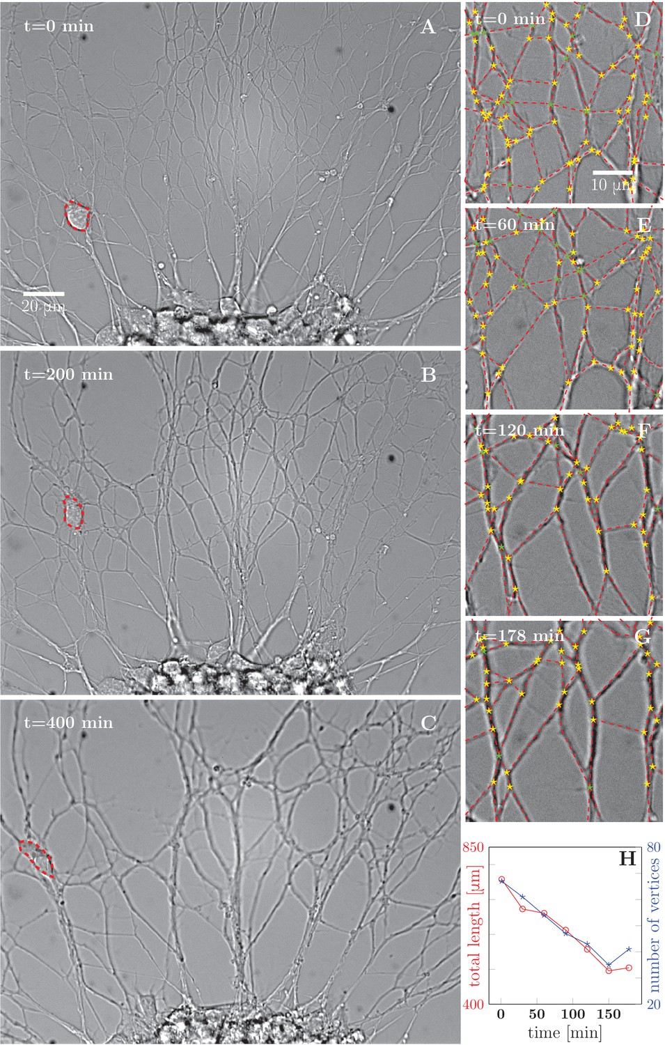
Progressive formation of fascicles in the evolving axon network.
(A–C) Evolution of the axonal network growing from an explant during 400-min time lapse recording, after 2 days of incubation; the red dashed outline delineates a travelling ensheating cell. Progressive coarsening of the network and decrease of total length and density can be seen. (D–G) Red dashed lines outline the edges of the network, while yellow stars indicate junctions between axons or axon bundles, and green stars indicate crossings. (H) Quantification of total length and number of vertices of the network area depicted in panels (D–G), as a function of time (based on seven manually segmented video frames). Segmentation coordinates for panels D-G and data from panel H data are available in Figure 1—source data 1.
-
Figure 1—source data 1
Segmentation coordinates (D–G), plot data (H).
- https://doi.org/10.7554/eLife.19907.004
Figure 1—figure supplement 1
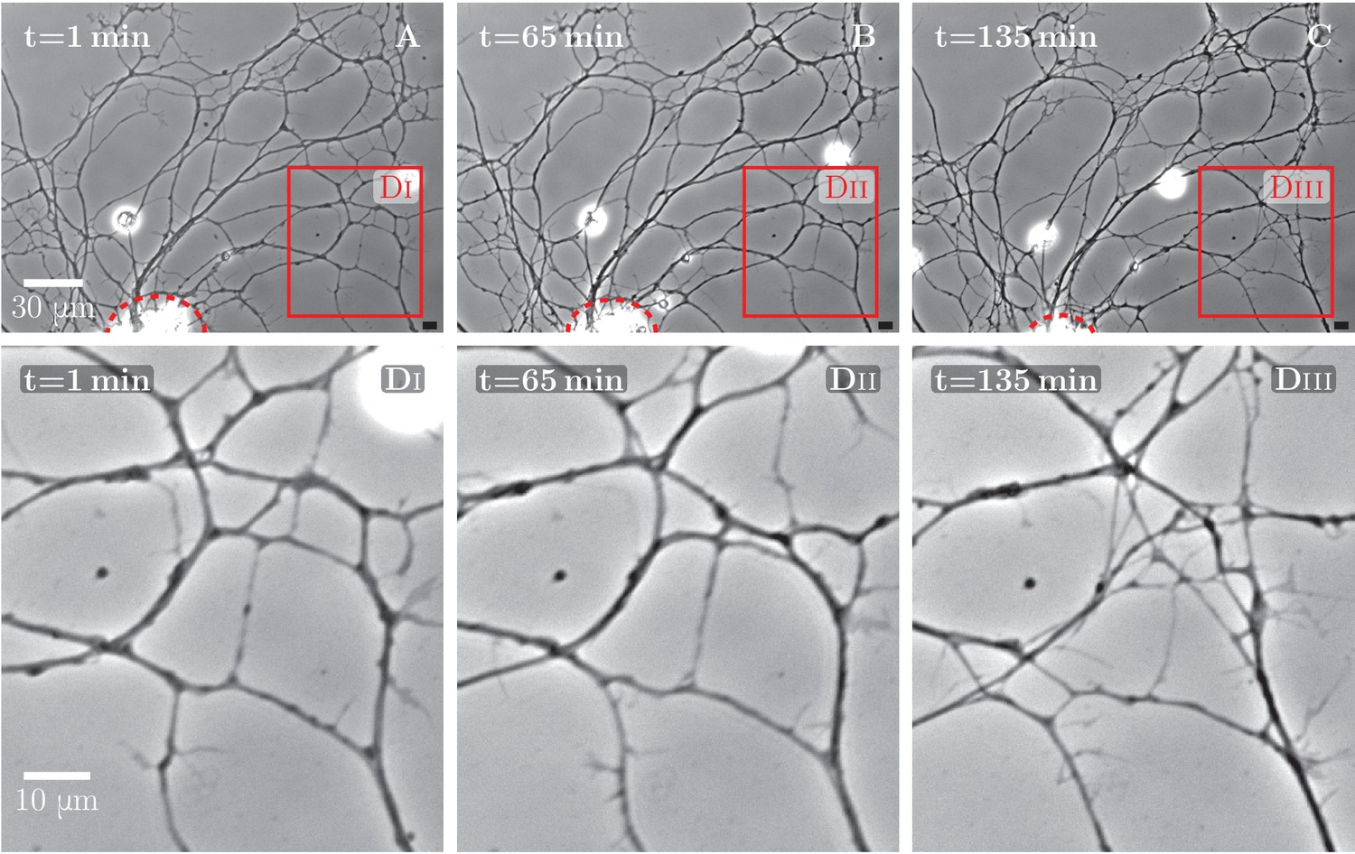
An example of spontaneous defasciculation correlated with explant contraction.
(A–C) Full field view of network evolution, from an experiment with no added drugs. The edge of the explant is marked by the red dashed line. After =65 min, the explant edge starts to move out of the field and pulls on the outgrown axon network. This causes defasciculation and an increase of network length in the area marked by the red square, labeled (Di–Diii). The panels (Di–Diii) show magnified views of the marked area. An increase in network density is apparent in the panel Diii. The time-lapse recording spanning =1 min through =135 min is provided as Figure 5—source data 1.
-
Figure 1—figure supplement 1—source data 1
Development of axon network over 135 min, with decoarsening visible in the lower right quadrant after =65 min, video corresponding to Figure 1—figure supplement 1.
- https://doi.org/10.7554/eLife.19907.006
Figure 2
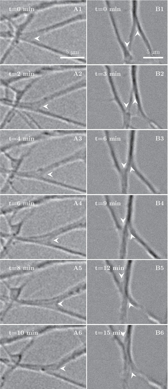
High-magnification images of individual axon zippers and their evolution in time.
Zipper vertices are marked by arrowheads. (A) advancing zipper, (B) two associated advancing zippers. The total length of the network segments in B decreases during the zippering process.
Figure 3
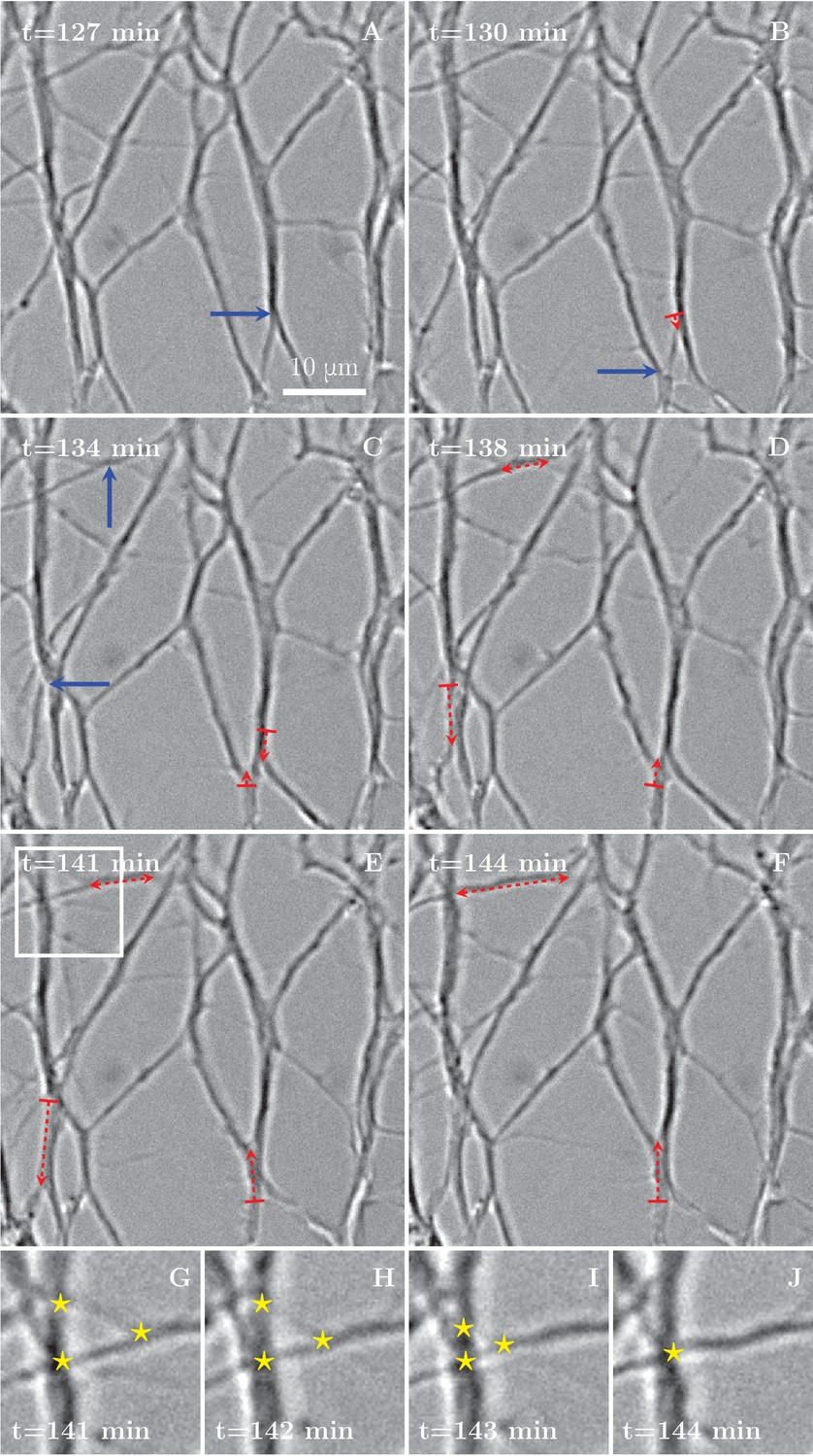
Zippering events drive the progressive formation of fascicles.
(A–F) Six frames extracted from the time sequence shown in Figure 1D–G. The blue arrows indicate vertices that will start to zippper in the following frame, the red dashed arrows illustrate the direction and the increase in length of the advancing zipper. If two arrowheads are present, there are two vertices extending a single segment. Frames G–J are enlargements of the inset in panel E in the period between the frames E and F, illustrating three vertices (marked by stars in frames G to I) merging into a single vertex (in frame J).
Figure 4 with 1 supplement
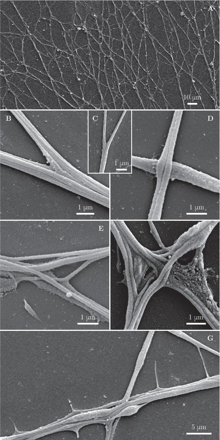
Fine morphological characterization of zippers with scanning electron microscopy.
Panel (A) illustrates a large area of the culture observed at low magnification. (B–C) illustrate a laminar vertex structure formed between small axon bundles (B) or between individual axons (C). (D) illustrates crossing of axons. (E) and (F) illustrate more complex, entangled vertices. Such configurations are unlikely to easily unzipper. (G) shows thin lateral protrusions, often seen along axon shafts. These protrusions can attach to nearby axons and pull on them.
Figure 4—figure supplement 1

Quantification of abundance of axon crossings, simple zippers and entangled zippers.
The SEM image was examined to assign simple zippers (mobile; marked in blue), entangled zippers (unable to recede; marked in red) and crossings of the axons (marked in green). The corresponding counts are indicated in the legend. The same type of analysis of a second SEM image provided the following results: 65 simple zippers, 37 entangled zippers and 24 crossings. Coordinates of selected points are available in Figure 4—figure supplement 1—source data 1..
-
Figure 4—figure supplement 1—source data 1
Coordinates of marked points.
- https://doi.org/10.7554/eLife.19907.012
Figure 5 with 1 supplement
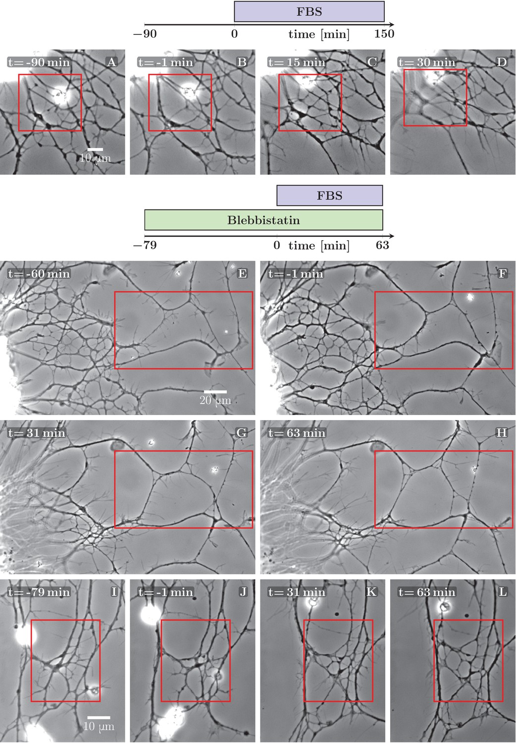
Defasciculation resulting from FBS-induced pull on the network.
The schemes indicate the protocol of drug addition for the experiments that are shown on the frames below the schemes. (A–D) FBS was added to the culture at =0 min. Decoarsening of part of the network (marked by the red rectangle) is visible. At a later stage, the network collapses. The full recording is provided as Figure 5—source data 1. (E–H) The culture was pretreated by blebbistatin added before =−60 min. Little change is visible between −60 and −1 min. At =0 min FBS is added, after which progressive movement of the explant border to the left can be observed, exerting a pulling force on the axons. As a result, unzippering occurs, the network defasciculates and several new loops appear in the area marked by the red rectangle. The full recording is provided as Figure 5—source data 2. (I–L) The culture was pretreated with blebbistatin (=−79 min) and the network remained mostly unchanged until FBS was added (=0 min). Defasciculation is visible in the frames K and L, where the area of interest is marked by the red rectangle. The full recording is provided as Figure 5—source data 3.
-
Figure 5—source data 1
Development of axon network over 240 min, treated with FBS at 90 min, video corresponding to Figure 5A–D.
- https://doi.org/10.7554/eLife.19907.014
-
Figure 5—source data 2
Development of axon network over 142 min, pretreated with blebbistatin, and treated with FBS at =79 min, video corresponding to Figure 5E-H.
- https://doi.org/10.7554/eLife.19907.015
-
Figure 5—source data 3
Development of axon network over 142 min, pretreated with blebbistatin, and treated with FBS at =79 min, video corresponding to Figure 5I-L.
- https://doi.org/10.7554/eLife.19907.016
Figure 5—figure supplement 1
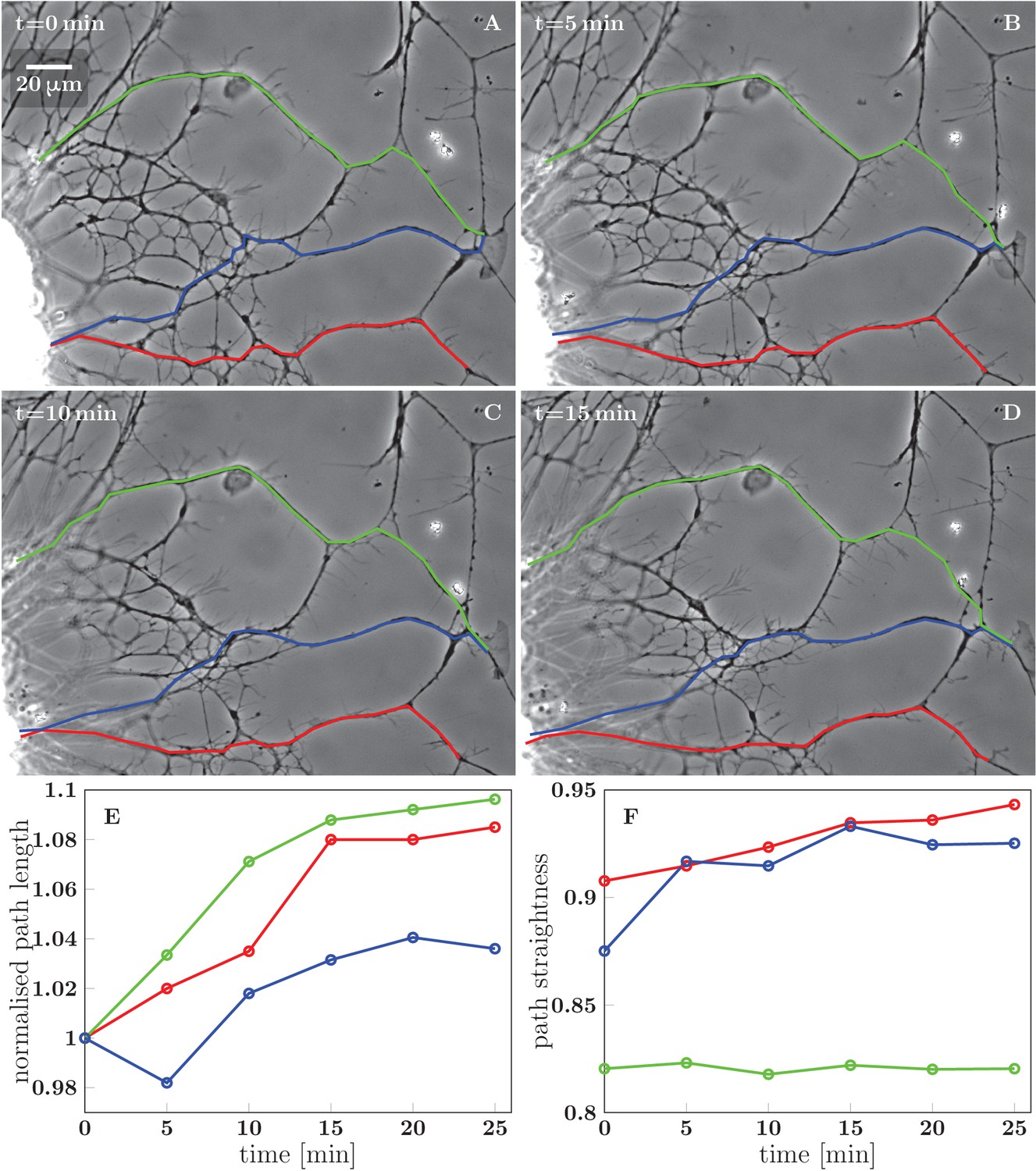
Stretching of the axons due to FBS-induced pull on the network.
(A–D) Network configurations in the first 15 min after FBS was added to the culture. Three candidate paths of axons growing from the right edge of the explant are marked in green, blue and red, with the green and blue paths terminating in a growth cone. (E) Time course of the total length of the three segmented paths, each normalized to the initial path length. (F) Time course of the path straightness, defined as the ratio of the direct-line distance between the initial and final points of the path to the total path length (i.e. straightness of 1 corresponds to a straight line). The colors of the datapoints in (E) and (F) correspond to the colors of the paths in (A–D). The straightness of the blue and red paths approaches 1.0, while the green path is prevented from such marked straightening by the immovable obstacle in the middle of the path. The coordinates of the path segments in panels (A–D) are available in Figure 5—figure supplement 1—source data 1.
-
Figure 5—figure supplement 1—source data 1
Coordinates of paths (A–D), plot data (E,F).
- https://doi.org/10.7554/eLife.19907.018
Figure 6
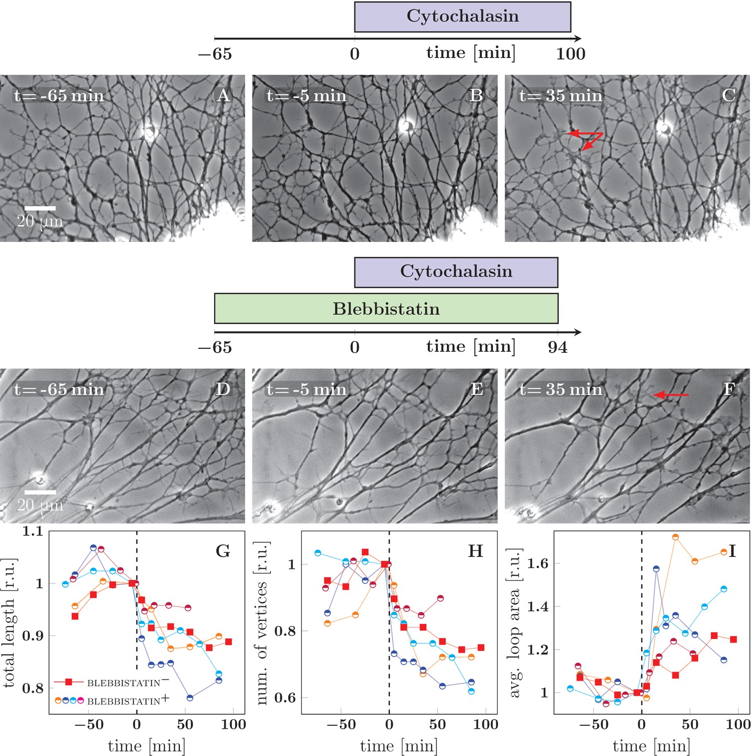
Cytochalasin-induced fasciculation of axon shafts.
The schemes indicate the protocol of drug addition for the experiments that are shown on the frames below the schemes. (A–C) Cytochalasin was added to the culture at =0 min. While there is little visible change between −65 and −1 min, the network exhibits coarsening between 0 and 35 min. The full recording is provided as Figure 6—source data 2. (D–F) The culture was pretreated with blebbistatin before =−65 min. Little change is visible between −65 and −1 min. After cytochalasin addition at =0 min, the culture exhibits coarsening. The full recording is provided as Figure 6—source data 3. The red arrows in frames C and F indicate prominent lamellipodia, which appear after the addition of cytochalasin. (G–I) The network statistics for the experiment of panel (A–C) (red squares), panel (D–F) (blue half-circles), and three other experiments with protocol equivalent to D–F, shown as Figure 6—source data 4 (orange half-circles), Figure 6—source data 5 (purple half-circles) and Figure 6—source data 6 (cyan half-circles). (G) Total length of the axon network in the field. (H) Total number of vertices of the axon network in the field. (I) Average area of cordless closed loop in the axonal network. The networks were manually segmented and analyzed as indicated in Materials and methods. In (G–I), the data was aligned by the time of cytochalasin addition marked =0 min and normalized by the value of the last measured timepoint before the drug was added. A sharp decrease of total length and of the number of vertices, as well as increase of average loop area, is seen within 30 min after =0 min, indicating coarsening of the network triggered by cytochalasin addition. Segmentation data and frames are available in Figure 6—source data 8 (please consult Materials and methods), source code used to generate the network statistics and input data is in Figure 6—source data 1, the data points plotted in panels G–I are in Figure 6—source data 7.
-
Figure 6—source data 1
ZIP archive; contains source code (Figure 6_source_code.m) and five ZIP archives with selection input data.
Running the code (with the five input archives in the same directory) performs data processing and statistical analysis, and outputs the data shown in plots G, H and I (see Materials and methods).
- https://doi.org/10.7554/eLife.19907.020
-
Figure 6—source data 2
Development of axon network over 165 min, treated with cytochalasin at =65 min, video corresponding to Figure 6A–C (red in graphs G–I).
- https://doi.org/10.7554/eLife.19907.021
-
Figure 6—source data 3
Development of axon network over 159 min, pretreated with blebbistatin, and treated with cytochalasin at =65 min, video corresponding to Figure 6D–F (blue in graphs G–I).
- https://doi.org/10.7554/eLife.19907.022
-
Figure 6—source data 4
Video of development of axon network over 159 min, pretreated with blebbistatin, and treated with cytochalasin at =65 min, orange data points in Figure 6G–I.
- https://doi.org/10.7554/eLife.19907.023
-
Figure 6—source data 5
Video of development of axon network over 129 min, pretreated with blebbistatin, and treated with cytochalasin at =67 min, purple data points in Figure 6G–I.
- https://doi.org/10.7554/eLife.19907.024
-
Figure 6—source data 6
Video of development of axon network over 166 min, pretreated with blebbistatin, and treated with cytochalasin at =75 min, cyan data points in Figure 6G–I.
- https://doi.org/10.7554/eLife.19907.025
-
Figure 6—source data 7
Plot data (G, H and I).
- https://doi.org/10.7554/eLife.19907.026
-
Figure 6—source data 8
ZIP archive; contains video frames and segmentation data underlying the analysis shown in the Figure 6G–I.
The archive contains analyzed frames (TIFF format) and corresponding segmentation selection data (ImageJ-generated ZIP archives). Data can be displayed using ImageJ, please refer to Materials and methods.
- https://doi.org/10.7554/eLife.19907.027
Figure 7
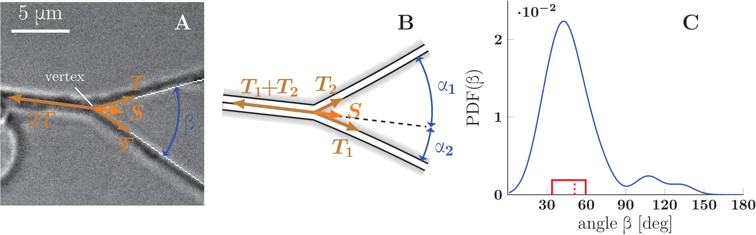
Force balance in static axon zippers.
(A) Illustration of a symmetric zipper. The zipper angle is marked in blue. The arrows denote the vectors of tension and axon-axon adhesive force . (B) illustration of an asymmetric zipper, the markings are the same as in A, but the tensions within the axons differ (). (C) distribution of initial and final equilibrium angles of measured zippers (17 zippers, 34 measurements) originating from four distinct cultures (each obtained from a different mother animal), transformed into a probability distribution using convolution with Normal kernel. The red dashed line marks the average angle value (51.2°) and the solid red box delimits the interquartile range (34°–60°). The values correspond to the full zipper angle , which equals in asymmetric case. Individual distributions of the angles , were not recorded, because of prevailing symmetry of measured zippers. The distribution includes only those zippers, which were stable at least 5 min before and after the dynamics. The measured angles and the distribution of panel C are available in Figure 7—source data 1.
-
Figure 7—source data 1
Estimated angle distribution (C) and underlying experimental angle data.
- https://doi.org/10.7554/eLife.19907.029
Figure 8 with 2 supplements
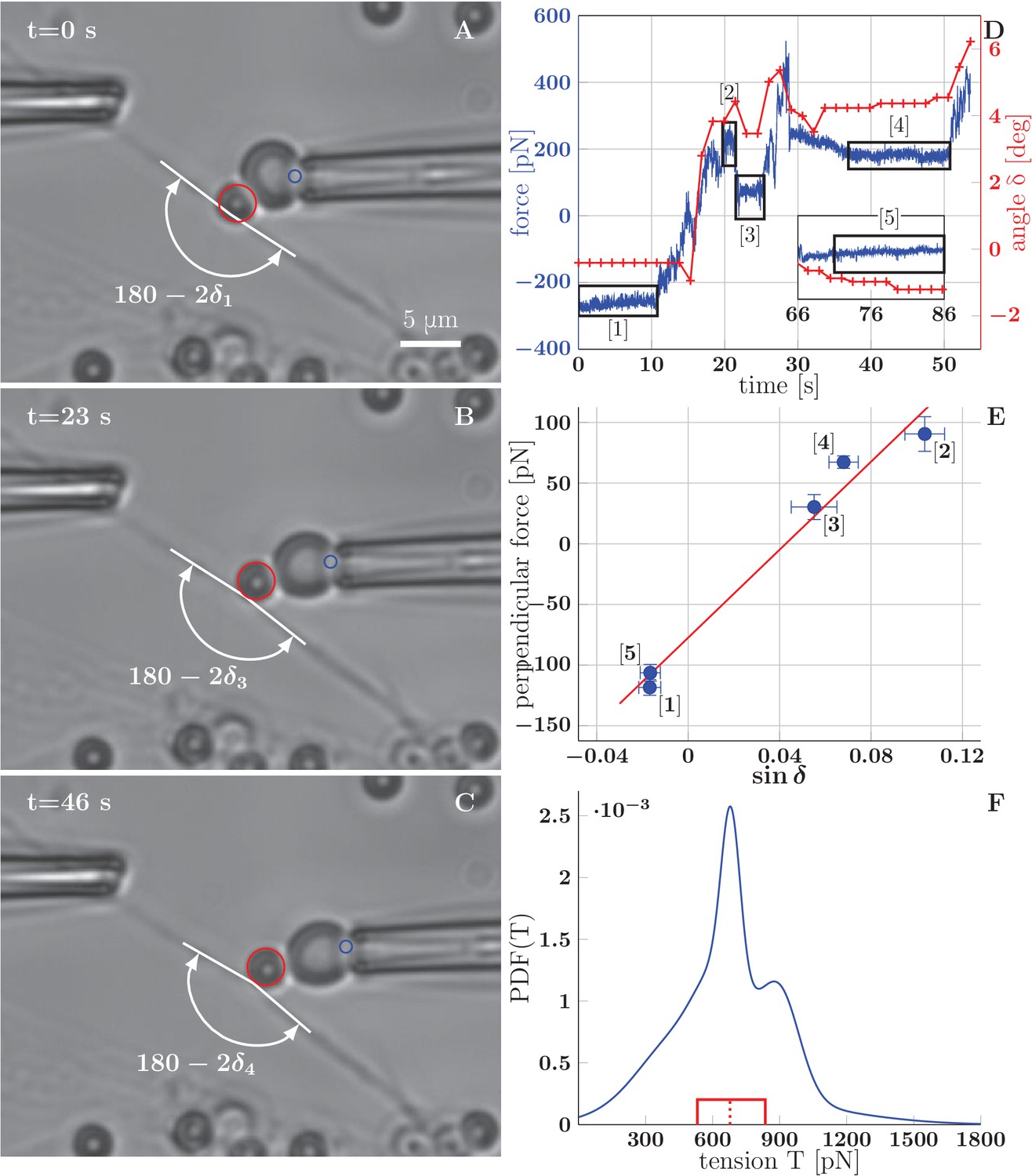
BFP measurements of axon tension.
(A–C) illustrate a BFP experiment (the full recording is in the video Figure 8–source data 1) . (A) The bead is slightly pushed against the axon (with deflection angle ), negative deformation (compression) of the RBC is recorded. (B,C) Different stages of the probe exerting a pulling force on the axon; the RBC undergoes positive deformation (extension), the axon deflection angle . Index of corresponds to the numbering of plateaux in panel D and data points in panel E. The tracked point on pipette and the tracked bead are marked by blue and red circles. (D) Time dependence of the force measured on the probe (evaluated for each frame at 65 fps), and the angle (evaluated each second). The deflection angle corresponds to deflection by pushing, means deflection by pulling. The deflection angle determines the lateral projection of axial tension acting at the apex, that is lateral tensile force . (E) Blue data points represent time-averaged qualities of individual plateaux (labelled by appropriate numbers), abscissa corresponds to average deformation and ordinate to average perpendicular probe force . The error bars represent a standard deviation of the quantities during each plateau. The red line is a linear fit of BFP data points, i.e. vs. , the slope corresponds to axon tension . Goodness of the fit is =0.97. (F) Distribution of axon tensions, calculated as a normalized sum of linear fit results from all BFP experiments—each fit was represented by a Normal distribution, with mean at given by the fit slope, and standard deviation , given by the standard deviation of the fit. The tension mode value is 678 pN, mean 679 pN (designated by the dashed red line), interquartile range (529–833) pN (delimited by the red box). The distribution of tension in based on =7 measurements, containing at least three force plateaux each, originating from four distinct cultures (each obtained from a different mother animal). The time course of force and angle (D), plateaux points and the fit (E), mean values of tension of all experiments and the distribution values (F) are available in the Figure 8—source data 2.
-
Figure 8—source data 1
Illustration of a BFP experiment with overlays that mark the results of pipette and bead tracking (Video).
- https://doi.org/10.7554/eLife.19907.031
-
Figure 8—source data 2
Time course of force and angle (D), plateaux averages and fit parameters (E), estimated tension distribution (F) and underlying experimental tension data.
- https://doi.org/10.7554/eLife.19907.032
Figure 8—figure supplement 1
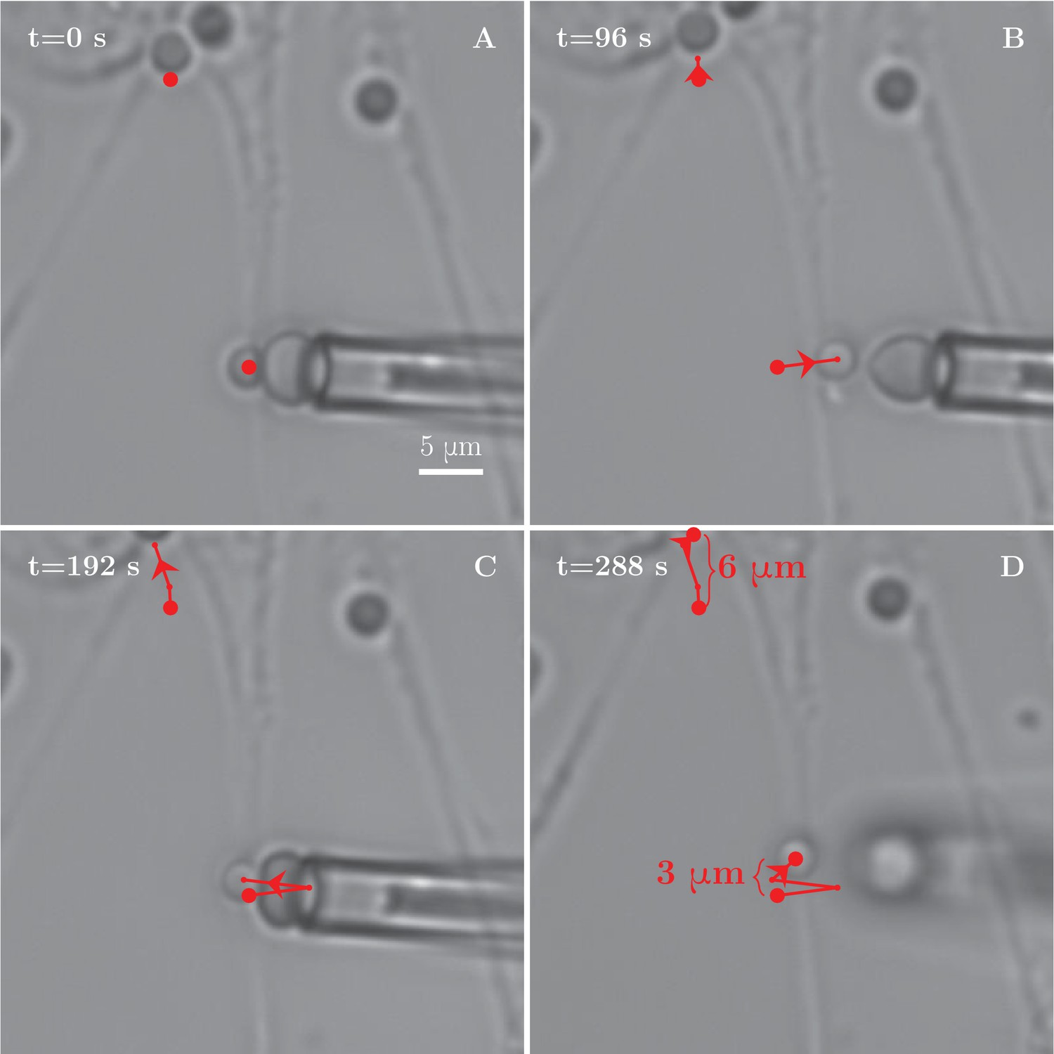
Tension increase during a BFP experiment with axon stretch.
(A) Axon stretching observed during a BFP manipulation experiment. The two red dots serve as tracer points. The explant in the upper part of the field gradually moves upwards, pulling the proximal section of the measured bundle along, while no immediate retraction of the rest of the bundle is observed. (B–D) Distance between the two points increases by 3 μm, demonstrating the stretching of the axon. The stretching is likely responsible for observed increase in tension within the axon between the frames (A–D). Comparing the tension measurements at the beginning of the video and at the later stages, we observe an increase from (432 ± 157) pN to (1665 ± 219) pN.
Figure 8—figure supplement 2
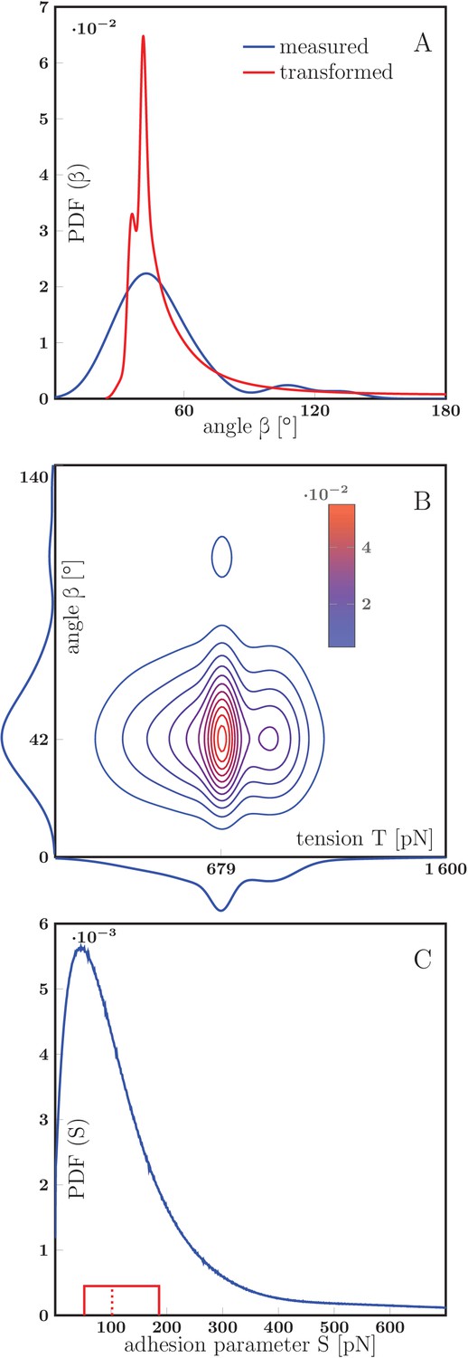
Estimation of the axon-axon adhesion parameter S.
(A) Distribution of static equilibrium angles measured from initial and final equilibria of measured zippers in vitro (blue line), and expected distribution of equilibrium angles based on transformation of the tension probability distribution (Equation 6 in Materials and methods) (red line). The adhesion parameter of the PDF()PDF() transformation was optimized to achieve maximal correlation between the distributions, with the result =88 pN and correlation coefficient 0.813. (B) Contour plot of the joint probability density of axon tension and static equilibrium vertex angle . The two distributions were considered independent, the joint probability is the product of marginal PDFs, which are shown along the corresponding coordinate lines. (C) Distribution of adhesion parameter , calculated by screening the values obtained from Equation 1 and the joint distribution in panel B. Interquartile range of is (52–186) pN (delimited by the solid red box), while the median of the distribution is 102 pN, designated by the dashed line. The data of experimental and transformed distributions of angles (A), experimental distributions of angles and tension (B) and probability distribution of adhesion coefficient (C) are available in Figure 8—figure supplement 2—source data 1, source code used to process the data is in Figure 8—figure supplement 2—source data 2..
-
Figure 8—figure supplement 2—source data 1
Data plotted in Figure 8—figure supplement 2A–C.
- https://doi.org/10.7554/eLife.19907.035
-
Figure 8—figure supplement 2—source data 2
Source code to process input data from Figure 8—figure supplement 2—source data 1.
- https://doi.org/10.7554/eLife.19907.036
Figure 9
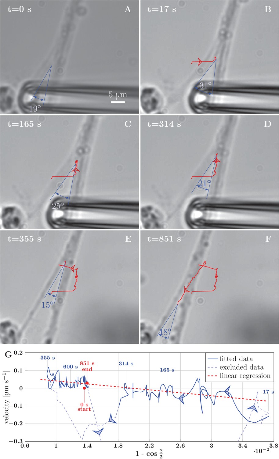
Example of induced unzippering and rezippering.
(A) Initial state of the zipper before the manipulation. (B) Angle increases as vertex shifts to the side with the initial pipette displacement. (C–D) The axons unzipper, slowly. (E) Pipette is removed and axon released, the vertex shifts strongly to the left to equilibrate the lateral force imbalance. (F) Axons zipper back toward the initial configuration. (G) Blue line (with time stamps) shows the velocity and angle of the vertex during the manipulation. Data points belonging to the full line were fitted using linear regression (dashed red line). The goodness of the fit is =0.48. The pale-blue dashed line corresponds to transients arising during manipulation (excluded from the regression). The values of angle were smoothed by a 20-frame Gaussian filter, and the velocity was calculated using convolution of positional data with derivative of the same Gaussian filter. The blue arrows show the direction of increasing time. Velocity, angle data and fit of panel G are available in Figure 9—source data 2.
-
Figure 9—source data 1
Induced unzippering experiment video corresponding to Figure 9.
- https://doi.org/10.7554/eLife.19907.038
-
Figure 9—source data 2
Velocity and angle data, fit parameters (G).
- https://doi.org/10.7554/eLife.19907.039
Figure 10
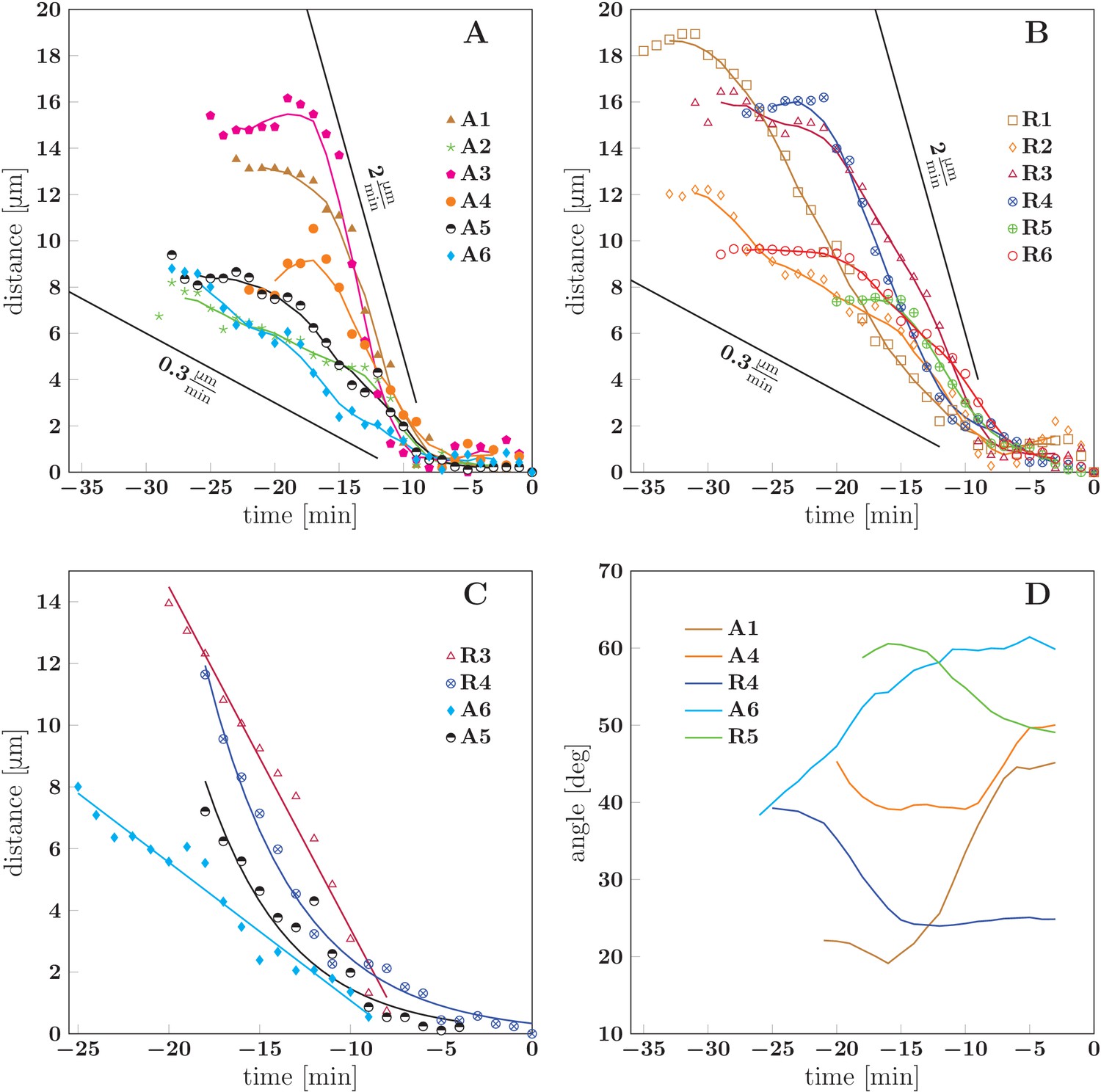
Dynamics of spontaneous zippering events in the evolving network.
(A) and (B) show the convergence to equilibrium for selected advancing and receding zippers, respectively. The distance between the zipper vertex location at the given time and the final equilibrium position is given. The lines with slopes delimit the typical zippering and unzippering velocities. (C) Fits illustrating approximately linear or exponential convergence in time. Linear fit equations: and ; exponential fit equations: and . (D) Time course of zipper angles, smoothed by five-frame window. Note that the angle increases for advancing zippers and decreases for receding zippers. Data plotted in panels A, B and D are available in Figure 10—source data 3.
-
Figure 10—source data 1
Video of receding zipper R4 from Figure 10.
- https://doi.org/10.7554/eLife.19907.043
-
Figure 10—source data 2
Video of receding zipper R5 from Figure 10.
- https://doi.org/10.7554/eLife.19907.044
-
Figure 10—source data 3
Plot data (A, B and D).
- https://doi.org/10.7554/eLife.19907.045
Figure 11

Geometry and notation for the dynamical model of axon zippering.
(A) Illustration for the zippering dynamics model. and denote the lengths of the two axons. The red dotted line represents the adhered zipper segment and its extension beyond the vertex (i.e. zipper axis), aligned with the -axis in the figure. The blue vector represents the conservative forces (i.e. tension and adhesion) and the red vector the resulting vertex velocity limited by friction. Projection of the velocity to the zipper axis, , determines the vertex-localized dissipative force, as . The strain rate, , determines the elongational viscous dissipative force, that is . (B) Illustration for the Appendix. represents a small displacement of the vertex. Vector is the velocity of the element , in contrast to the velocity of the vertex, , in panel A. Axial and transverse substrate friction forces and are proportional to the element velocity components and .
Figure 12

Predicted zippering dynamics resulting from applying a perturbation to a zipper initially in equilibrium, converging to a new equilibrium.
(A) The landscape of tensile and adhesive energy (Equation 7) for the new equilibrium condition (specified by the parameter values: left tension , right tension (up from in the initial equilibrium), axon-axon adhesion ). Blue contours indicate locations of equal energy. Gray dashed lines show axons in the final equilibrium, dashed red line is the gradient trajectory between equilibria,. The full lines indicate zipper vertex trajectories following a rapid increase of the right tension. Red: trajectory with dominant substrate friction (), blue: trajectory with dominant zippering friction (), black: trajectory with dominant elongation friction (). The trajectories with dominant friction types are represented by the same color code across all panels. (B) The same trajectories as in A, with time stamps. The tension in the right axon increased rapidly over 5 s and then was kept constant (see green line in panel D). (C) Trajectories during gradual perturbation, with dominant zippering friction (blue), substrate friction (red) and elongation friction (black) over 1000 s. The tension was gradually growing in the right axon over 500 s and then was kept constant (see green line in panel E). (D, E) velocity of vertex during transition, color code corresponds to panels B and C, green line represents the prescribed tensile force in the right axon during the transition. For each model run, one friction constant was set to a particular value to probe its effect on the trajectory, others were set to zero. The following values were used: axial substrate friction =200 Pa s, transverse substrate friction =200 Pa s, elongation friction =3000 nN s, zippering friction (in this case, a small substrate friction value ==1 Pa s was introduced to avoid a singularity when the motion direction was perpendicular to the zippering axis). Source code of the implemented zipper model used to generate the data is available in Figure 12—source data 1.
-
Figure 12—source data 1
Source code of zipper dynamical model to generate plot data (A–E).
- https://doi.org/10.7554/eLife.19907.048
Figure 13
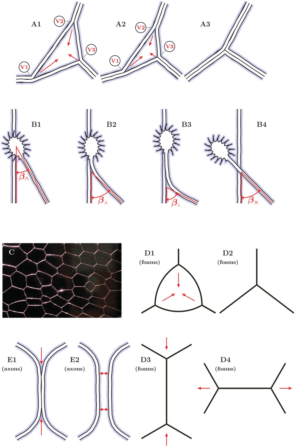
Elementary dynamical processes in fasciculating axon networks and in coarsening liquid foams (froths).
(A1–A3) Two vertices are lost during the process of closing of a loop formed by three axon segments. The initial configuration starts to zipper at one or more vertices, gradually decreasing the total network length. A single junction formed by three pairs of fully zippered axons remains. (B1–B4) Possible outcomes of initial contact of two axons. (B1) Growth cone (GC) interacts with the shaft of another axon, (B2) small initial incidence angle allows incoming GC to adhere and follow the shaft, (B3) the two shafts zipper, increasing the contact angle, (B4) if the initial incidence angle exceeds the equilibrium zipper angle, no stable zippered segment can be formed and the growth cone crosses over. (C) Photograph of structure formed by a liquid foam restricted between two glass plates. The gas bubbles are separated by liquid walls that meet at triple junctions. (D1–D4) Schemes illustrating the elementary topological processes in liquid foams. (D1) A three-sided bubble with curved walls, containing gas under excess pressure. (D1–D2) The gas diffuses to neighboring cells and the three-sided bubble gradually collapses. This process is called T2. (D3–D4) In foams, the T1 process leads to a reconnection of bubble walls, preserving the number of vertices of the network. (E1–E2) In the axon network, separation rather than reconnection results from unzippering. (E1) Two vertices delimiting a zippered segment start to recede, (E2) Once the adhered segment length decreases to zero, the two axons detach and separate (see experimental example in Video 2). Panel C is adapted from https://commons.wikimedia.org/wiki/Category:Foam\#/media/File:2-dimensional_foam.jpg:Foam\#/media/File:2-dimensional_foam.jpg by Klaus-Dieter Keller, released into the public domain by the author.
Figure 14
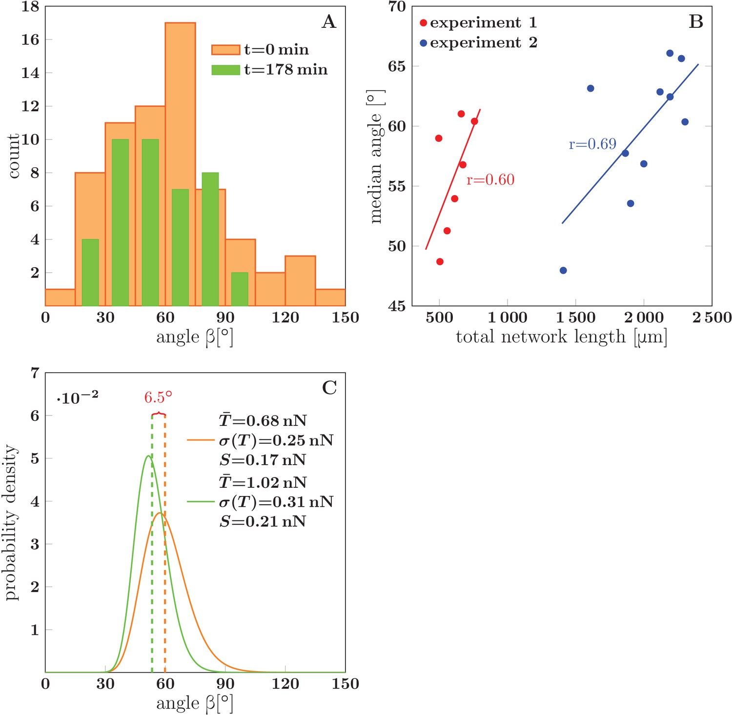
Evolution of the network distribution of zipper angles.
(A) The distribution of zipper angles in the network configurations of Figure 1D (=0 min, total 66 vertices) and Figure 1G (=178 min, total 44 vertices). (B) Correlation between median angle and the total network length in two experiments; denotes the Pearson correlation coefficient. (C) Predicted equilibrium zipper angle distribution PDF() obtained as a transformation of distribution of fascicle tension PDF() using Equation 6 (see main text and Materials and methods). The distribution of tensions was approximated by a lognormal distribution PDF. The distribution plotted in orange corresponds to the values of tension from BFP experiments, =0.68 nN, =0.25 nN, and adhesion parameter =0.17 nN adjusted to match the initial median angle of experiment 1. The distribution plotted in green corresponds to parameters rescaled with mean fascicle size as , , , with increase in mean fascicle size () corresponding to Figure 1D–G (see main text). The change in median angle in panel C is 6.5°, as compared to 7.5° given by the trendline in panel B (experiment 1). The data of histograms (A), correlations (B) and distributions (C) are available in Figure 14—source data 1. The source code used to generate distributions in panel C is available in Figure 14—source data 2.
-
Figure 14—source data 1
Data of histograms (A), correlations (B) and distributions (C).
- https://doi.org/10.7554/eLife.19907.051
-
Figure 14—source data 2
Source code to generate angle distributions (C) using Equation 6, see Materials and methods.
- https://doi.org/10.7554/eLife.19907.052
Figure 15
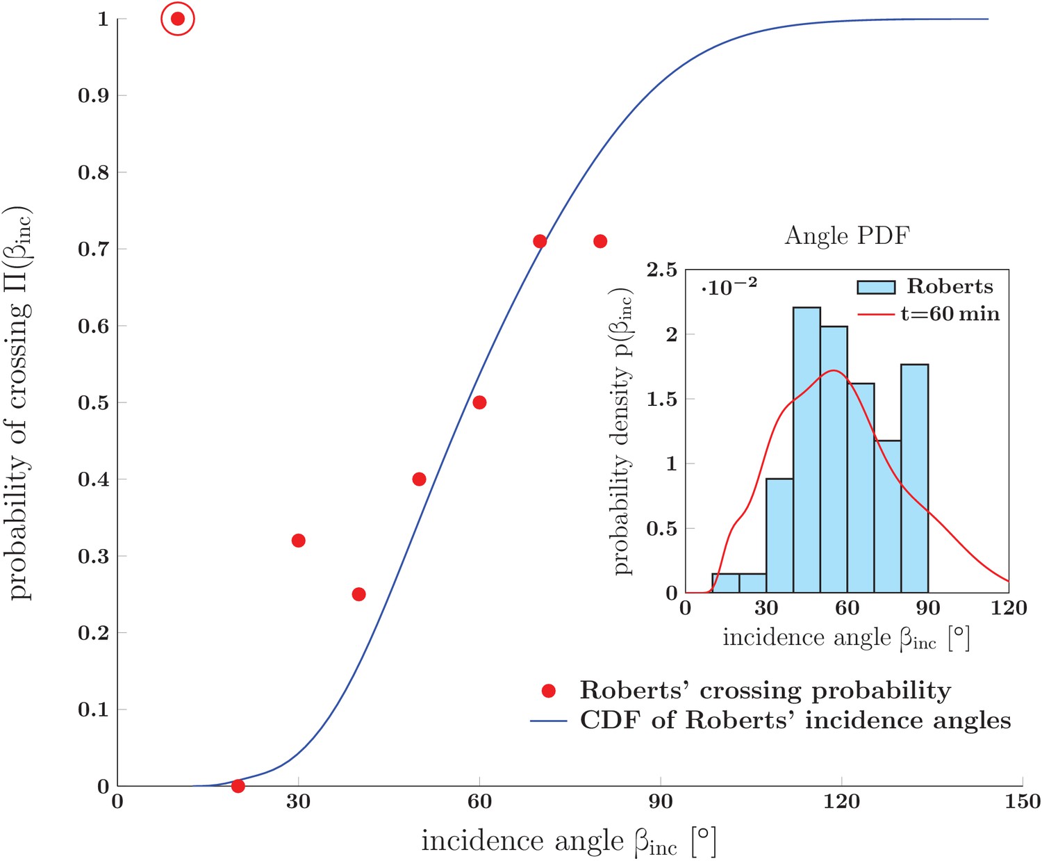
Prediction for the probability of crossing (rather than zippering) of two neurites, and its comparison to in vivo experimental data.
The red dots show data from Fig. 14 of Ref. (Roberts and Taylor, 1982) (referred to as Roberts in the figure): the observed probability of crossing of two neurites as function of observed incidence angle . The blue line is the cumulative distribution function of angles of incidence obtained from Roberts' data. It was calculated as , where the PDF of angles of incidence, , was constructed by kernel-smoothing the Roberts’ histogram. The crossing probability of interval (0–10)° is an outlier (marked by the red ring) based on a single observed case. Inset: Histogram of angles of incidence as observed by Roberts (upper panel of Fig. 13 in Roberts and Taylor (1982)) . The red line is the PDF of vertex angles measured in our in vitro system (Figure 1 at 60 min). The crossing probabilities and angles, experimental data and the distributions, are available in Figure 15—source data 1.
-
Figure 15—source data 1
Crossing probabilities and angles—data (Roberts and Taylor, 1982) and distributions estimates.
- https://doi.org/10.7554/eLife.19907.054
Videos
Video 1
Development and coarsening of axon network over 12 h, corresponding to Figure 1.
https://doi.org/10.7554/eLife.19907.007
Video 2
Induced unzippering of a zipper segment delimited by two vertices on either side.
In this case the unzippering becomes complete and the two constitutive bundles separate.
Video 3
Induced unzippering experiment.
In this case the vertex does not recede, despite the large increase in zipper angle resulting from the manipulation by micropipette.
Video 4
Growth cone losing grip on the substrate.
https://doi.org/10.7554/eLife.19907.055Download links
A two-part list of links to download the article, or parts of the article, in various formats.
Downloads (link to download the article as PDF)
Open citations (links to open the citations from this article in various online reference manager services)
Cite this article (links to download the citations from this article in formats compatible with various reference manager tools)
Axon tension regulates fasciculation/defasciculation through the control of axon shaft zippering
eLife 6:e19907.
https://doi.org/10.7554/eLife.19907


