Non-coding cancer driver candidates identified with a sample- and position-specific model of the somatic mutation rate
- Aarhus University Hospital, Denmark
- Aarhus University, Denmark
Figures
Figure 1 with 1 supplement
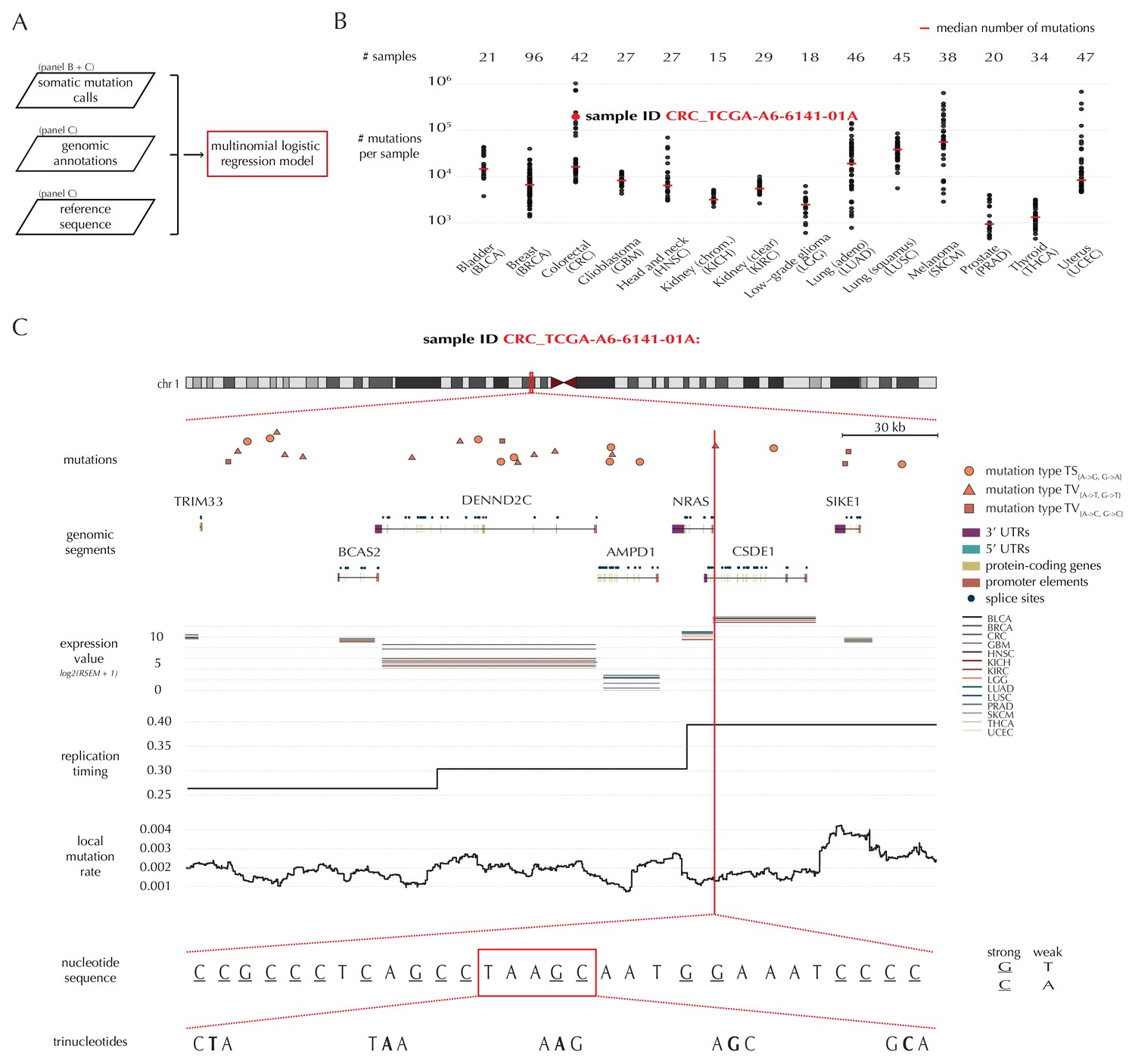
Variation in mutation rate at different scales and various explanatory variables.
(A) The flowchart illustrates the input to the model fit that predicts the position- and sample-specific mutational probabilities. (B) The number of mutations observed per sample divided into the 14 different cancer types. (C) The set of genomic annotations used as explanatory variables are illustrated on a 300 kb region of chromosome 1 for the colorectal cancer sample CRC_TCGA-A6-6141-01A. For illustrative purposes, the nucleotide sequence is shown on a 30 bp section of chromosome 1 and trinucleotides likewise on a 5 bp section.
-
Figure 1—source data 1
The number of mutations observed for each of the 505 samples.
This data set relates to Figure 1B.
- https://doi.org/10.7554/eLife.21778.004
Figure 1—figure supplement 1
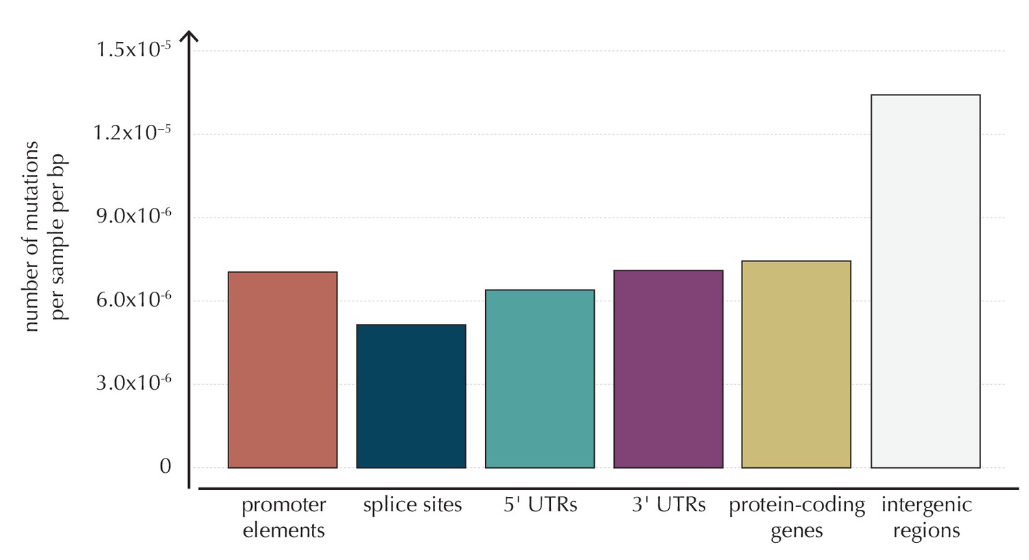
The average number of mutations observed per sample per bp for each of the considered element types, as well as for intergenic regions.
https://doi.org/10.7554/eLife.21778.005-
Figure 1—figure supplement 1—source data 1
The number of mutations per sample per bp for the defined element types.
This data set relates to Figure 1—figure supplement 1.
- https://doi.org/10.7554/eLife.21778.006
Figure 2
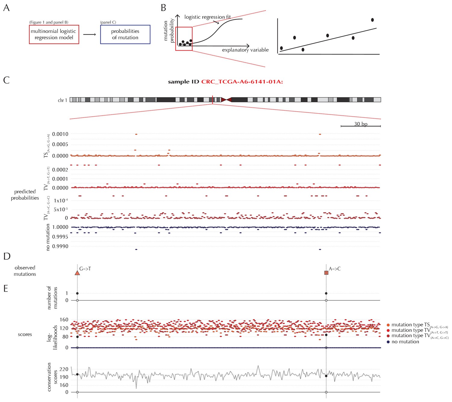
Position- and sample-specific predicted mutation rates and scoring-schemes.
(A) A multinomial logistic regression model is used to predict the sample- and position-specific background mutation-probabilities. (B) The genomic annotations and the reference sequence (Figure 1) are used as explanatory variables in a regression fit of the somatic mutation rate. In effect, a logistic regression model is fitted for each of the four types of outcome (three types of mutation and no mutation) and combined into a multinomial logistic regression fit. Logistic regression ensures probability-predictions between zero and one. The mutation probabilities are of such small magnitude that we observe near linearity of the logistic regression curve. (C) Sample- and position-specific predicted mutation probabilities for each of the four outcomes in a 300 bp region of chromosome 1 (chr1:115,824,535–115,824,834) for the colorectal cancer sample CRC_TCGA-A6-6141-01A. (D) Observed sample-specific somatic mutations within the same region. For the sample in question, two mutations are observed; one of type TV{A→T, G→T} and one of type TV{A→C, G→C}. (E) Sample- and position-specific scores for each of the three considered scoring schemes.
Figure 3 with 1 supplement
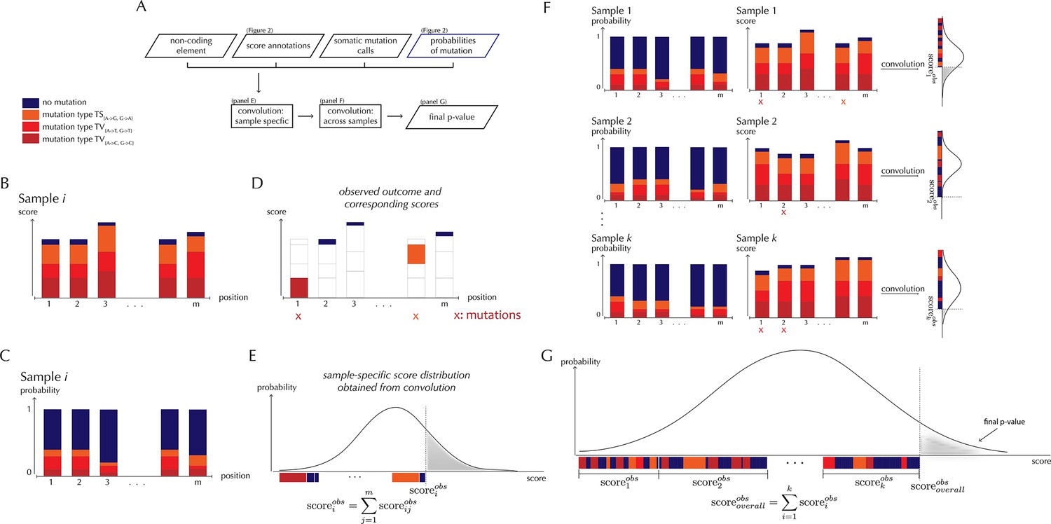
ncdDetect analysis concepts.
(A) Flowchart of the algorithmic steps of ncdDetect. Panels B through E show the sample-specific calculations, while panels F and G show the calculations across samples. (B) The genomic candidate region is annotated with position- and sample-specific scores. The values of these scores depend on the choice of scoring scheme. (C) The region is also annotated with sample- and position-specific predicted mutation probabilities. These probabilities are predicted by the null model and does not depend on the choice of scoring scheme. (D) The observed score of the sample is defined as the sum of the scores associated with the observed mutational events. Scores based on number of mutations and conservation will assign non-mutated positions with a score-value of zero. Scores based on log-likelihoods will assign non-mutated positions with a positive score-value, which in practice will be near zero. (E) The sample-specific background score-distribution is obtained by convolution. (F) Sample-specific calculations are carried out for each individual sample in the dataset. (G) The overall background score-distribution is obtained by convolution of the individual-sample distributions. This figure is conceptual and not based on actual data. Figure 4D–F are real examples of background score-distributions.
Figure 3—figure supplement 1
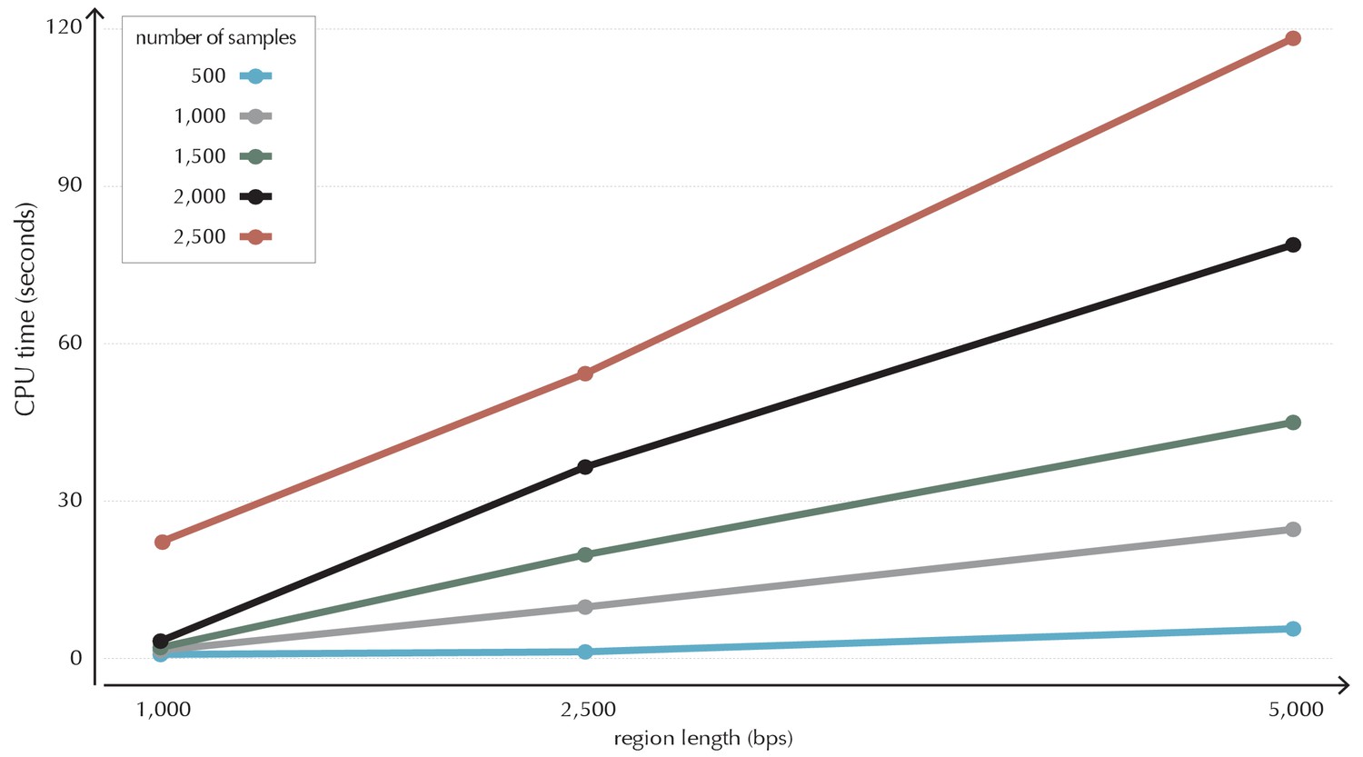
Illustration of time complexity of the ncdDetect algorithm.
Each point illustrates the CPU time in seconds used to calculate the background score distribution for a candidate region of a given length for a given number of samples.
Figure 4 with 2 supplements
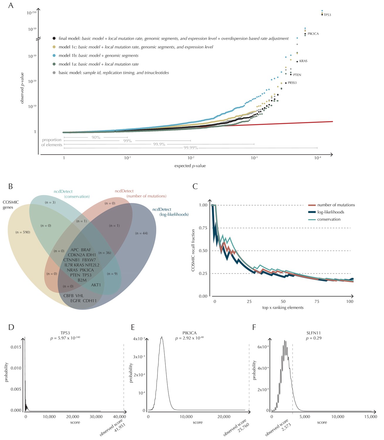
Analysis of protein-coding genes to evaluate ncdDetect performance.
(A) The final null model is obtained through forward model-selection. The QQ-plot shows the p-values of all genes (n = 19,256) plotted against their uniform expectation under the null for each of the five models considered. Deviations from the expectations (red identity line) are seen for a varying proportion of the genes (0.5–10%). Results are shown for conservation scores. Similar plots for log-likelihoods and number of mutations are shown in Figure 4—figure supplement 1. (B) Venn diagram showing the overlap between protein-coding genes called as drivers by ncdDetect (q<0.10) for the three scoring schemes and the COSMIC Gene Census list. (C) COSMIC Gene Census recall plot. The fraction of COSMIC genes recalled in the top ncdDetect candidates. (D–F) The two most significant genes called by ncdDetect are TP53 and PIK3CA. An example of a gene not called significant is SLFN11. For each of these, the convoluted background score-distributions are shown together with the observed scores and resulting p-values.
-
Figure 4—source data 1
P-values obtained on protein-coding genes for each of the five models considered.
The p-values are obtained using conservation scores. This data set relates to Figure 4A.
- https://doi.org/10.7554/eLife.21778.012
-
Figure 4—source data 2
COSMIC Gene Census recall data.
The fraction of recalled COSMIC genes in the top ncdDetect candidates, for the three different scoring schemes. This data set relates to Figure 4C.
- https://doi.org/10.7554/eLife.21778.013
-
Figure 4—source data 3
The background score distribution for the protein-coding gene TP53 obtained with conservation scores.
This data set relates to Figure 4D.
- https://doi.org/10.7554/eLife.21778.014
-
Figure 4—source data 4
The background score distribution for the protein-coding gene PIK3CA obtained with conservation scores.
This data set relates to Figure 4E.
- https://doi.org/10.7554/eLife.21778.015
-
Figure 4—source data 5
The background score distribution for the protein-coding gene SLFN11 obtained with conservation scores.
This data set relates to Figure 4F.
- https://doi.org/10.7554/eLife.21778.016
Figure 4—figure supplement 1

Analysis of protein-coding genes to evaluate ncdDetect performance for scores defined by log-likelihoods and the number of mutations.
The final null model is obtained by forward model selection. The QQ-plots show the p-values of all genes (n = 19,256) plotted against their uniform expectation under the null for each of the models considered. (A) Results using log-likelihoods. (B) Results using number of mutations. The corresponding plot for conservation scores are shown in Figure 4A.
-
Figure 4—figure supplement 1—source data 1
P-values obtained on protein-coding genes for each of the models considered.
The p-values are obtained using log-likelihoods and number of mutations as scores. This data set relates to Figure 4—figure supplement 1.
- https://doi.org/10.7554/eLife.21778.018
Figure 4—figure supplement 2
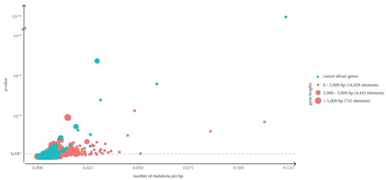
The p-values (based on conservation scores) plotted as a function of the total number of mutations across samples observed per bp for all protein-coding genes.
The point size indicates gene length. The mean number of mutations per bp is on average eight times higher for the COSMIC genes detected by ncdDetect compared to the undetected COSMIC genes.
-
Figure 4—figure supplement 2—source data 1
For each protein-coding gene, the gene length, the number of observed mutations across all 505 samples, and the p-value obtained using conservation scores are given.
Furthermore, the COSMIC status is indicated. This data set relates to Figure 4—figure supplement 2.
- https://doi.org/10.7554/eLife.21778.020
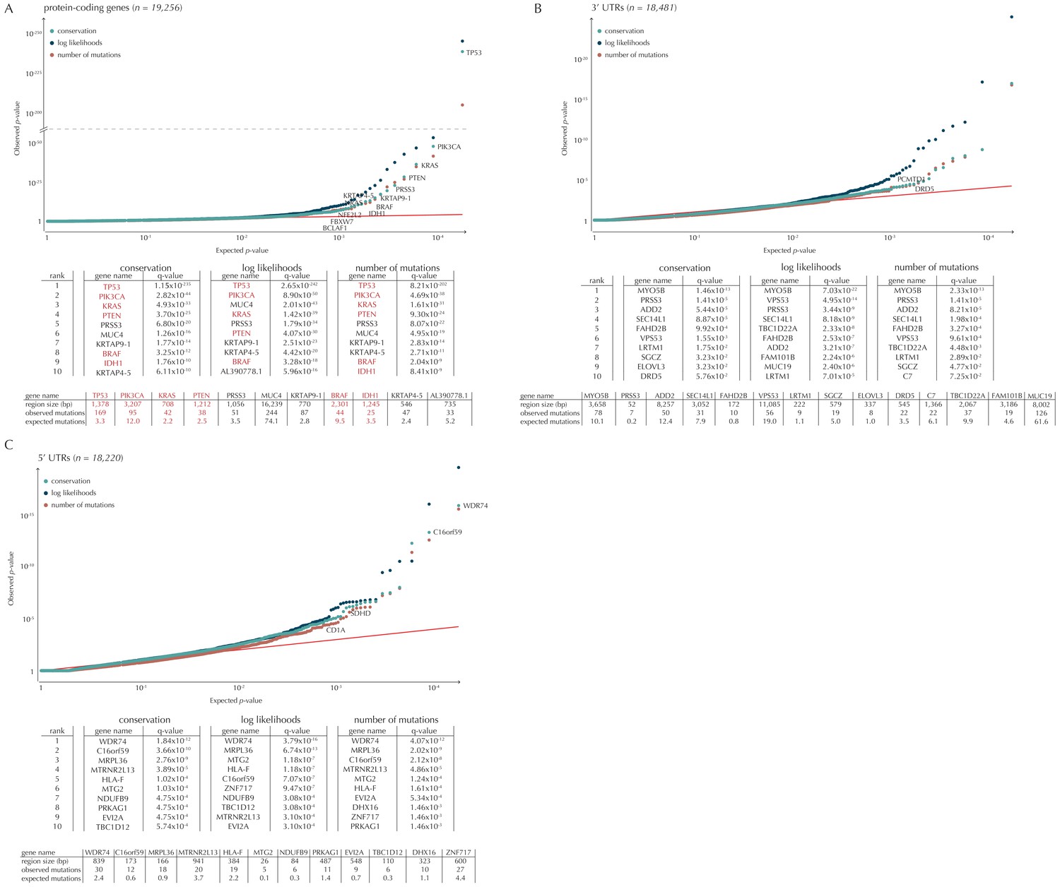
Figure 5 with 3 supplements
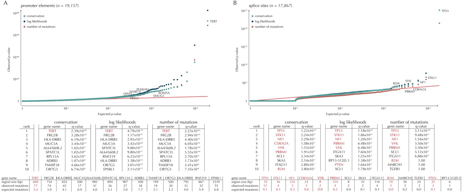
Q-values and top-ten ranking non-coding elements for each of the three proposed scoring schemes.
The results discussed in the text relate to conservation scores. Non-coding elements associated to COSMIC genes are highlighted in red. For each element, the region size is given together with the observed number of mutations and the expected number of mutations under the null model. (A) The QQ-plot shows the p-values for all promoter elements (n = 19,157) plotted against their uniform expectation under the null. One hundred and sixty promoter elements are found to be significant. (B) QQ-plot of p-values for all splice sites (n = 17,867). The p-values do not follow the expectation under the null. This is explained by the fact that 90% of all splice sites carry no mutations. Three splice sites come up significant with ncdDetect after correcting for multiple testing.
-
Figure 5—source data 1
P-values obtained on promoters and splice sites using conservation scores.
This data set relates to Figure 5A–B. P-values obtained using log-likelihoods and number of mutations as scores are in Supplementary files 2–3.
- https://doi.org/10.7554/eLife.21778.022
Figure 5—figure supplement 1
Q-values and top-ten ranking elements for each of the three proposed scoring schemes.
Protein-coding COSMIC genes, or non-coding elements associated to COSMIC genes, are highlighted in red. For each element, the region size is given together with the observed number of mutations and the expected number of mutations under the null model. (A) The QQ-plot shows the p-values for all protein-coding genes (n = 19,256) plotted against their uniform expectation under the null. Sixty-four protein-coding genes are found to be significant (conservation scores). (B) QQ-plot of p-values for all 5’ UTRs (n = 18,220). In total, 86 5’ UTRs are significant. (C) QQ-plot of p-values for all 3’ UTRs (n = 18,481), of which 16 are found to be significant. The complete sets of significant elements for each region type are given in Supplementary files 1–3. Similar plots for promoter elements and splice sites are shown in Figure 5.
-
Figure 5—figure supplement 1—source data 1
P-values obtained on protein-coding genes, 3’ UTRs and 5’ UTRs using conservation scores.
This data set relates to Figure 5—figure supplement 1A–C. P-values obtained using log-likelihoods and number of mutations as scores are in Supplementary files 2–3.
- https://doi.org/10.7554/eLife.21778.024
Figure 5—figure supplement 2
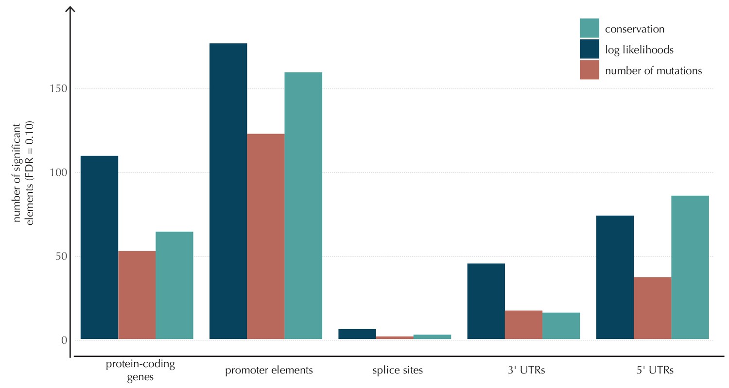
The number of elements called significant for each of the three proposed scoring schemes, for each of the defined element types.
The use of log-likelihoods results in the highest number of elements called significant across most element types, and the use of the number of mutations results in the fewest.
-
Figure 5—figure supplement 2—source data 1
The number of elements called significant for each of the three proposed scoring schemes, for each of the defined element types.
This data set relates to Figure 5—figure supplement 2.
- https://doi.org/10.7554/eLife.21778.026
Figure 5—figure supplement 3
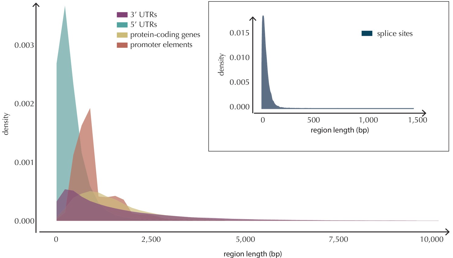
Length distributions of all defined element types.
https://doi.org/10.7554/eLife.21778.027-
Figure 5—figure supplement 3—source data 1
The length of each of the analyzed elements.
This data set relates to Figure 5—figure supplement 3.
- https://doi.org/10.7554/eLife.21778.028
Figure 6 with 1 supplement
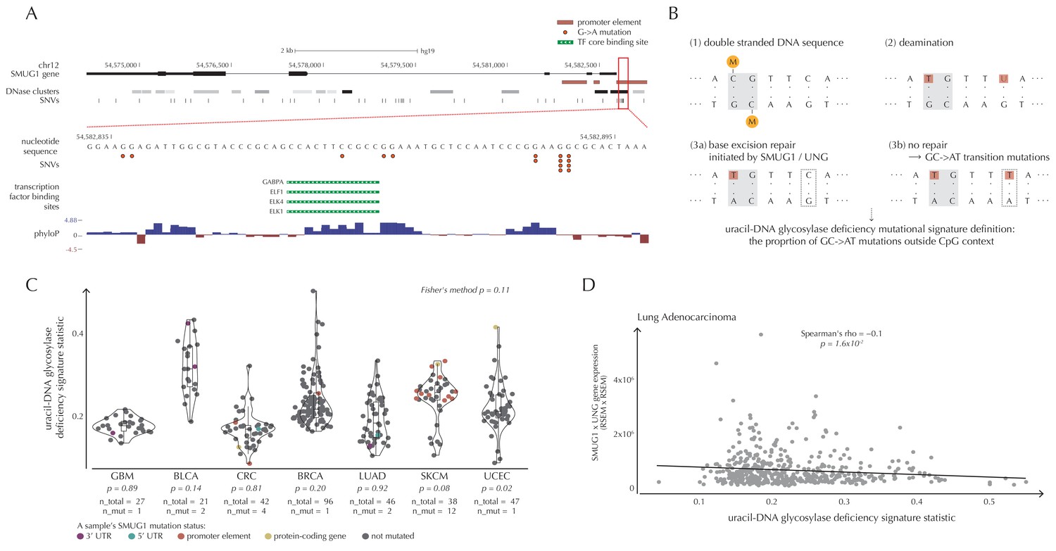
SMUG1 mutations and base excision repair.
(A) Genomic overview of SMUG1 showing its promoter region (Kent et al., 2002). The DNase clusters track shows DNase hypersensitive regions where the darkness is proportional to the maximum signal strength observed in any cell line (ENCODE Project Consortium, 2012). The transcription-factor-binding sites (TFBSs) track shows core regions of transcription factor binding (Gerstein et al., 2012). The phyloP track shows evolutionary conservation of positions (Pollard et al., 2010). (B) Uracil-DNA glycosylase deficiency signature definition: (1) Cytosines may be methylated (orange circles) at CpG sites (gray box). (2) Spontaneous deamination (red boxes) of non-methylated cytosine results in uracil, causing U:G mismatches. Spontaneous deamination of methylated cytosine results in thymine, causing T:G mismatches. (3a) SMUG1 and UNG are uracil-DNA glycosylases, which, via base excision repair, will repair the U:G mismatches caused by deamination. (3b) If unrepaired, the U:G mismatches will result in G→A mutations. (C) A one-sided Wilcoxon rank sum test is performed per cancer type to investigate if samples with a SMUG1 mutation have a higher value of the uracil-DNA glycosylase deficiency signature statistic than samples without such a mutation. The analysis is based on the 505 whole genome TCGA samples. Each dot represents a sample, and the color represents the SMUG1-associated mutated element. (D) Correlation between the uracil-DNA glycosylase deficiency signature statistic and the product of SMUG1 and UNG gene expression using TCGA exome data for lung adenocarcinoma.
-
Figure 6—source data 1
The defined uracil-DNA glycosylase deficiency signature statistic for each sample of the cancer types GBM, BLCA, CRC, BRCA, LUAD, SKCM and UCEC.
For each sample, the SMUG1 mutation status is indicated. This data set relates to Figure 6C.
- https://doi.org/10.7554/eLife.21778.030
-
Figure 6—source data 2
The defined uracil-DNA glycosylase deficiency signature statistic, as well as SMUG1 gene expression, UNG gene expression, and SMUG1xUNG gene expression for TCGA exome samples.
Expression values are RSEM values. This data set relates to Figure 6D as well as Figure 6—figure supplement 1.
- https://doi.org/10.7554/eLife.21778.031
Figure 6—figure supplement 1
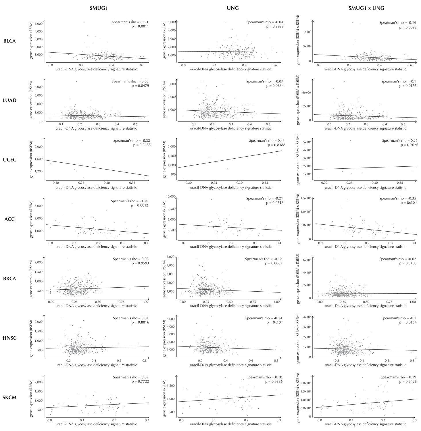
Examples of correlation between the uracil-DNA glycosylase deficiency signature statistic and SMUG1 gene expression (first column), UNG gene expression (second column) and the product of SMUG1 and UNG gene expression (third column) using TCGA exome data for seven different cancer types (rows).
The correlation is assessed using one-sided Spearman’s correlation tests. For some cancer types, the correlation coefficients are positive, although these cases are not significant and generally based on few samples.
Figure 7
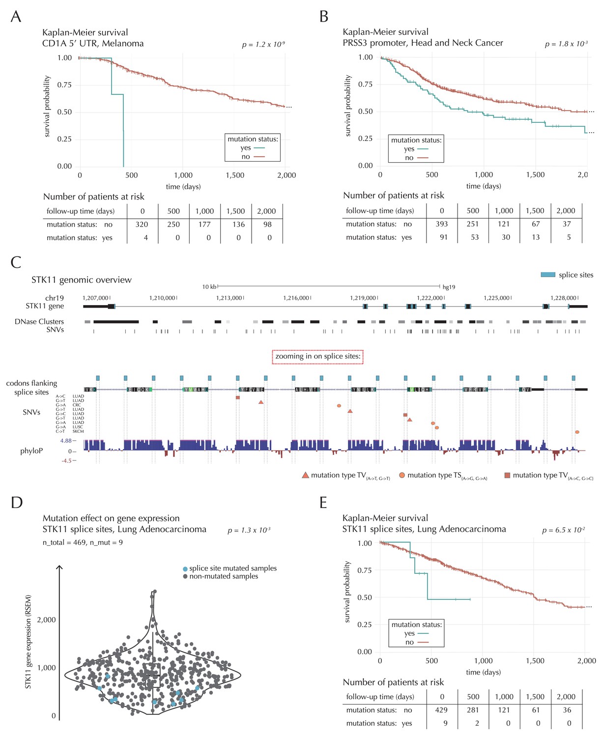
Survival- and expression analysis of CD1A, PRSS3 and STK11 mutations.
(A) Kaplan-Meier survival curves for melanoma samples with and without mutations in the 5’ UTR of CD1A. For illustration purposes, the data are shown for a follow-up time of 2000 days, at which point 98 out of 324 patients (30%) are still at risk. The analysis is based on the TCGA exome sample set. (B) Kaplan-Meier survival curves for HNSC patients with and without PRSS3 promoter mutations. The data are shown for a follow-up time of 2000 days, at which point 42 out of 484 patients (9%) are still at risk. The analysis is based on the TCGA exome sample set. (C) Genomic overview of STK11, zooming in on its combined splice sites region. The phyloP track shows evolutionary conservation of positions. (D) A two-sided Wilcoxon rank sum test is performed for LUAD samples from the TCGA exome sample set, to investigate if samples mutated in the splice site region of STK11 have a different gene expression level than samples without such mutations. (E) Kaplan-Meier survival curves for LUAD samples with and without STK11 splice site mutations. The data are shown for a follow-up time of 2000 days, at which point 36 out of 438 patients (8%) are still at risk. The analysis is based on the TCGA exome sample set.
-
Figure 7—source data 1
STK11 mutation status and STK11 gene expression (RSEM) for 469 LUAD TCGA exome samples.
This data set relates to Figure 7D.
- https://doi.org/10.7554/eLife.21778.034
Appendix 1—figure 1
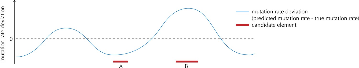
Illustration of the motivation behind the overdispersion-based rate adjustment.
For candidate element A, we overestimate the mutation rate, and thus end up with a conservative p-value for this element when analysing it with ncdDetect. For candidate element B, on the other hand, we underestimate the mutation rate. In this case, ncdDetect will produce a p-value that is too small, creating a potential false-positive call. The effect of underestimating the mutation rate will be greater for longer candidate elements.
Appendix 1—figure 2

QQ-plots of p-values obtained with and without the overdispersion-based rate adjustment.
(A) QQ-plots of all protein-coding genes (excluding TP53 for illustration purposes). (B) QQ-plots of protein-coding genes shorter than 700 bp. For the shorter genes, the p-values are not particularly inflated. The overdispersion-based rate adjustment does not affect the distribution of p-values much. (C) QQ-plots of protein-coding genes longer than 3000 kb. For the longer genes, the p-values are inflated, and the overdispersion-based rate adjustment effectively corrects for much of this inflation.
-
Appendix 1—figure 2—source data 1
P-value and gene length for each protein-coding gene.
The p-values are obtained with and without the overdispersion-based rate adjustment. This data set relates to Appendix 1—figure 2.
- https://doi.org/10.7554/eLife.21778.044
Appendix 1—figure 3
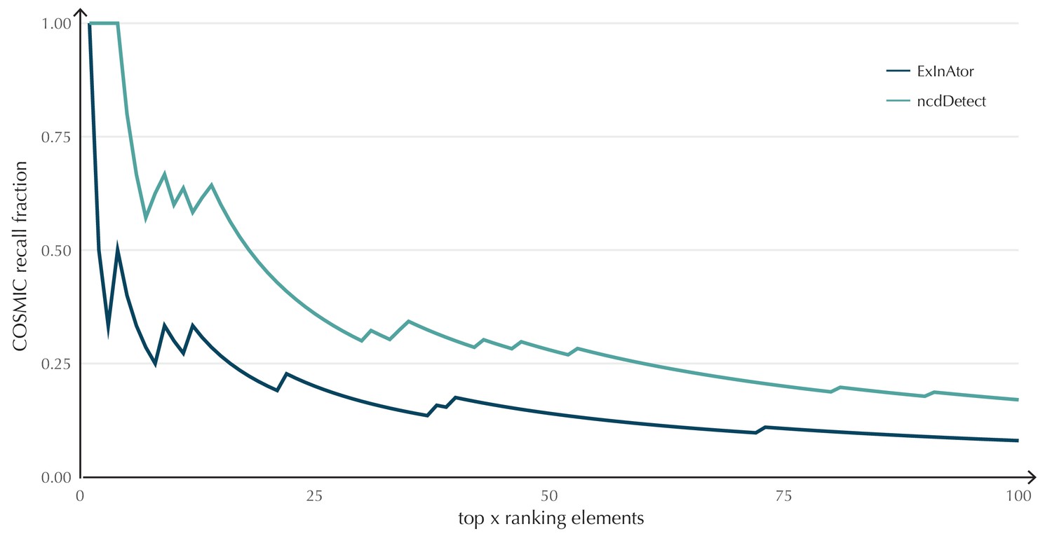
COSMIC Gene Census recall plot.
The fraction of COSMIC genes recalled in the top ncdDetect and ExInAtor candidates.
-
Appendix 1—figure 3—source data 1
COSMIC Gene Census recall data.
The fraction of recalled COSMIC genes in the top ncdDetect and ExInAtor candidates. This data set relates to Appendix 1—figure 3.
- https://doi.org/10.7554/eLife.21778.046
Appendix 1—figure 4
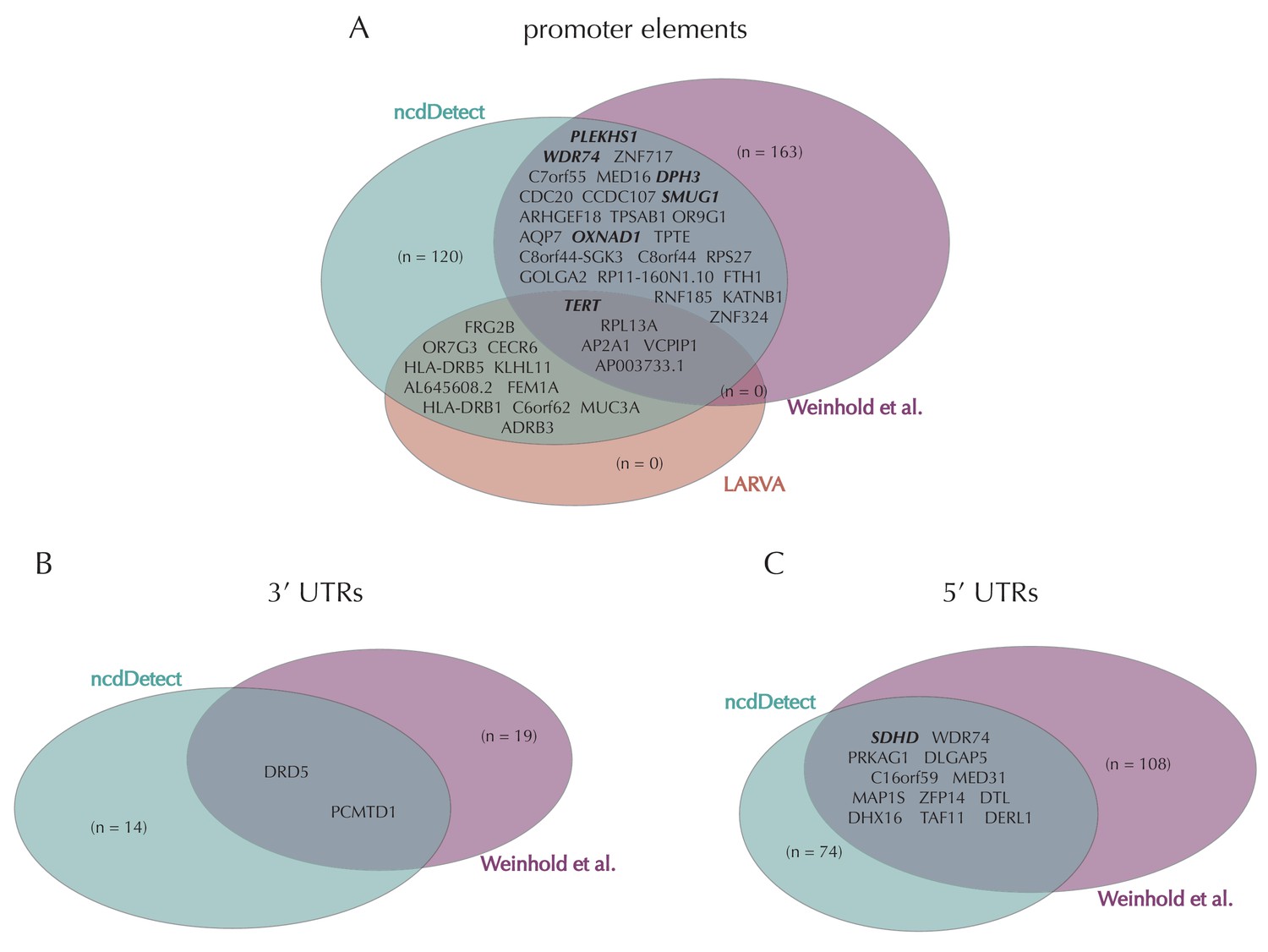
Illustration of overlap between significant elements found by ncdDetect and other non-coding cancer driver screens.
Highlighted elements are mentioned in the text. (A) Overlap of promoter elements found to be significant with ncdDetect and LARVA, as well as promoter elements previously described in a non-coding cancer driver screen (Weinhold et al., 2014). We note that TERT and PLEKHS1 are also detected by a second non-coding driver screen (Melton et al., 2015). (B) Overlap between 3' UTRs detected by ncdDetect and 3' UTRs detected by a previous study (Weinhold et al., 2014). (C) Overlap between 5' UTRs detected by ncdDetect and 5' UTRs detected by a previous study (Weinhold et al., 2014). We note, that out of the 863 whole genomes analyzed in (Weinhold et al., 2014), 356 are sequenced by the TCGA. These samples appear to be a subset of the 505 TCGA samples analyzed here. The data sets are thus not completely independent.
Author response image 1
Tables
Table 1
Overview of elements analyzed with ncdDetect. Regions located on chromosome X and Y are excluded from the analyses (Material and methods: Candidate elements).
| Element type | Number of elements | Median element length (bps) | Percentage of genome covered |
|---|---|---|---|
| protein-coding genes | 20,153 | 1296 | 1.19 |
| promoter elements | 20,052 | 848 | 0.69 |
| splice sites | 18,682 | 30 | 0.03 |
| 3’ UTRs | 19,346 | 1007 | 1.06 |
| 5’ UTRs | 19,078 | 259 | 0.25 |
Appendix 1—table 1
Analysis of the top 15 ncdDetect protein-coding candidates.
| Rank | Gene name | q-value | Size (bp) | Cosmic | Conclusion |
|---|---|---|---|---|---|
| 1 | TP53 | 1.15 × 10−235 | 1378 | True | Putative cancer driver gene |
| 2 | PIK3CA | 2.82 × 10−44 | 3207 | True | Putative cancer driver gene |
| 3 | KRAS | 4.93 × 10⁻³³ | 708 | True | Putative cancer driver gene |
| 4 | PTEN | 3.70 × 10⁻²⁵ | 1212 | True | Putative cancer driver gene |
| 5 | PRSS3 | 6.80 × 10⁻²⁰ | 1056 | False | Reported cancer association |
| 6 | MUC4 | 1.26 × 10⁻¹⁶ | 16,239 | False | Likely false positive due to length |
| 7 | KRTAP9-1 | 1.77 × 10⁻¹⁴ | 770 | False | Reported cancer association |
| 8 | BRAF | 3.25 × 10⁻¹² | 2301 | True | Putative cancer driver gene |
| 9 | IDH1 | 1.76 × 10⁻¹⁰ | 1245 | True | Putative cancer driver gene |
| 10 | KRTAP4-5 | 6.11 × 10⁻¹⁰ | 546 | False | Reported cancer association |
| 11 | NRAS | 2.20 × 10⁻⁸ | 570 | True | Putative cancer driver gene |
| 12 | AL390778.1 | 5.95 × 10⁻⁸ | 735 | False | No reported cancer driver properties |
| 13 | NFE2L2 | 3.15 × 10⁻⁷ | 1890 | True | Putative cancer driver gene |
| 14 | FBXW7 | 7.35 × 10⁻⁷ | 2618 | True | Putative cancer driver gene |
| 15 | BCLAF1 | 7.92 × 10⁻⁶ | 2763 | False | Reported cancer association |
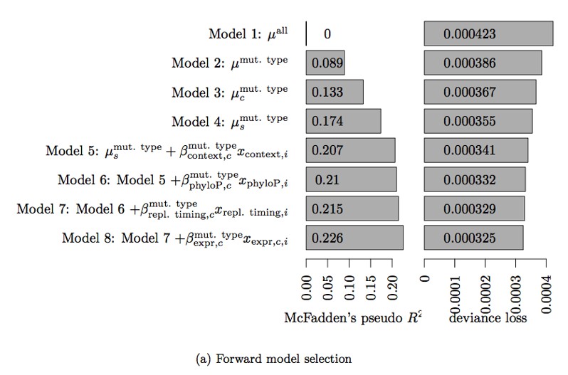
Author response table 1
Table 3. Deviance loss and McFadden’s pseudo R2 for each of the models tested in Step 3 to obtain model 8.
| Model | Deviance loss | McFadden’s pseudo R2 |
|---|---|---|
| Model 7 + | 0.0003248 | 0.2258 |
| Model 7 + | 0.0003279 | 0.2154 |
| Model 7 + | 0.0003289 | 0.2154 |
| Model 7 + | 0.0003289 | 0.2152 |
| Model 7 + | 0.0003290 | 0.2150 |
| Model 7 + | 0.0003291 | 0.2150 |
Additional files
-
Supplementary file 1
Supplementary results.
P-values obtained with ncdDetect using conservation scores.
- https://doi.org/10.7554/eLife.21778.035
-
Supplementary file 2
Supplementary results.
P-values obtained with ncdDetect using log likelihood scores.
- https://doi.org/10.7554/eLife.21778.036
-
Supplementary file 3
Supplementary results.
P-values obtained with ncdDetect using number of mutations as scores.
- https://doi.org/10.7554/eLife.21778.037
-
Supplementary file 4
Region definitions.
Definitions of candidate elements: Promoter regions, splice sites, 3’ UTRs, 5’ UTRs and protein-coding genes.
- https://doi.org/10.7554/eLife.21778.038
-
Supplementary file 5
Expression analyses and a uracil-DNA glycosylase deficiency signature statistic.
General expression analyses results and analyses performed to investigate the impact of SMUG1 mutations on expression levels as well as the uracil-DNA glycosylase deficiency signature statistic.
- https://doi.org/10.7554/eLife.21778.039
-
Supplementary file 6
Correlation between mutation status and survival.
Data overview and results obtained from the survival analyses.
- https://doi.org/10.7554/eLife.21778.040
-
Supplementary file 7
Information on how to access expression and survival TCGA data sets.
Overview of the specific TCGA samples included in the expression and survival analyses.
- https://doi.org/10.7554/eLife.21778.041
-
Appendix 1—figure 2—source data 1
P-value and gene length for each protein-coding gene.
The p-values are obtained with and without the overdispersion-based rate adjustment. This data set relates to Appendix 1—figure 2.
- https://doi.org/10.7554/eLife.21778.044
-
Appendix 1—figure 3—source data 1
COSMIC Gene Census recall data.
The fraction of recalled COSMIC genes in the top ncdDetect and ExInAtor candidates. This data set relates to Appendix 1—figure 3.
- https://doi.org/10.7554/eLife.21778.046
Download links
A two-part list of links to download the article, or parts of the article, in various formats.
Downloads (link to download the article as PDF)
Open citations (links to open the citations from this article in various online reference manager services)
Cite this article (links to download the citations from this article in formats compatible with various reference manager tools)
Non-coding cancer driver candidates identified with a sample- and position-specific model of the somatic mutation rate
eLife 6:e21778.
https://doi.org/10.7554/eLife.21778


