Nonlinear feedback drives homeostatic plasticity in H2O2 stress response
- Institut de Génétique et de Biologie Moléculaire et Cellulaire, France
- Centre National de la Recherche Scientifique, France
- Institut National de la Santé et de la Recherche Médicale, France
- Université de Strasbourg, France
- IBITECS, SBIGEM, CEA-Saclay, France
- University of Gothenburg, Sweden
Figures
Figure 1 with 2 supplements
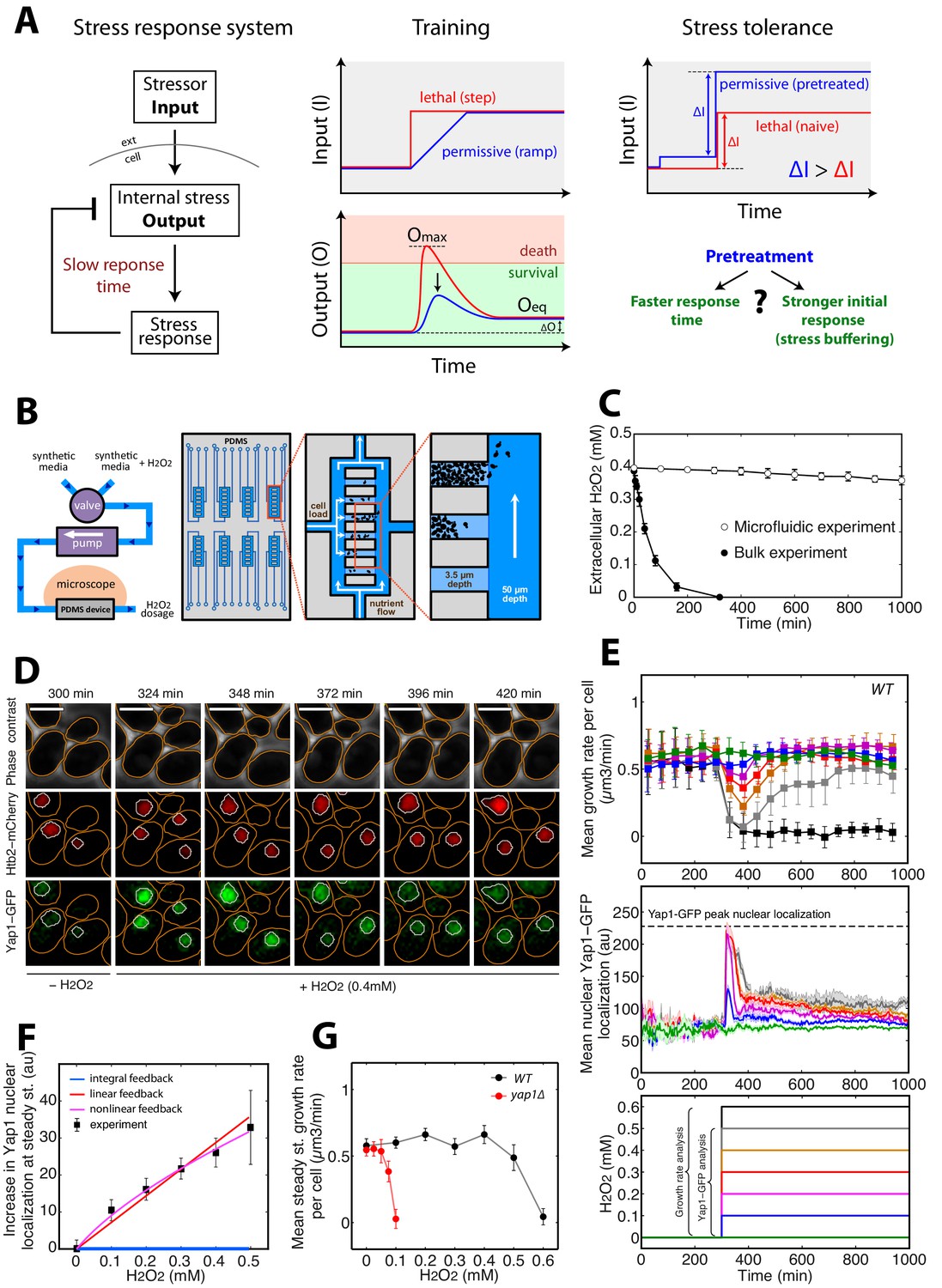
A single-cell microfluidics assay to monitor yeast adaptation to H2O2.
(A) Schematic representation of ‘training’ and ‘stress tolerance’ phenomena in a simple negative feedback-based system. (B) Schematic of the microfluidic device setup for live-cell imaging in H2O2-containing media. (C) Decline in extracellular H2O2 concentration comparing the single-cell assay and bulk experiment (starting at cellular OD600 = 0.5). (D) Sequence of phase-contrast and fluorescence images of cells at the indicated time points after addition of 0.4 mM H2O2 at t = 300 min. The red and green channels represent the Htb2-mCherry (nuclear marker) and Yap1-GFP signals, respectively. Orange and white lines represent the cellular and nuclear contours obtained after automated segmentation. The white bars represent 5 µm. (E) Top: Mean growth rate per cell as a function of time after addition of different H2O2 concentrations at t = 300 min, as indicated in the bottom panel. Middle: Mean nuclear Yap1-GFP localization as a function of time, with the same color coding as in the top and bottom panels. Yap1-GFP scoring is not possible at 0.6 mM due to metabolic arrest/cell death and GFP signal decline. (F) Increase in mean Yap1-GFP localization (relative to the pre-stress level) at steady state (measured for t > 800 min) as a function of H2O2 concentration added at t = 300 min during a step experiment. Lines represent the best fits to mathematical models of integral (blue), linear (red) and nonlinear (magenta) feedback with different sets of assumptions (see Materials and methods). (G) Comparison of growth rate at steady state as a function of H2O2 concentration for the wild-type (WT) strain and the Δyap1 mutant. Error bars and shaded regions are SEM (C, N = 6; E, N > 100 for most time points; F and G, N > 100 for each H2O2 concentration). See also Figure 1—figure supplement 1 and Materials and methods.
Figure 1—figure supplement 1

Medium diffusion properties in the microfluidics device.
(A) Fluorescein diffusion kinetics in an empty trapping cavity. Top left: phase-contrast image centered on a trapping cavity with two supply channels on the sides. The blue circle corresponds to the region of interest (ROI) of the supply channel in which the GFP signal is scored over time (bottom left: blue line). The red circle corresponds to the ROI of the trapping cavity in which the GFP signal is scored over time (bottom left: red line). Right: fluorescence images were taken at the indicated time points. The white bar represents 5 µm. (B) Same experiment as (A) for a crowded cavity. The magnification region on the right bottom corner (GFP and phase contrast) shows that the fluorescein doesn’t enter the cells during the experiment. The white bar represents 5 µm. (C) Scoring of the mean nuclear Yap1-GFP localization as a function of time for cells located at the edge of the trapping cavity (30 s time resolution). Error bars are SEM (N > 100 for all time points). (D) Phenotypic distribution across the cells depending of their position in the trapping cavity. p-Value is calculated using a Chi-squared test of independency.
Figure 1—figure supplement 2
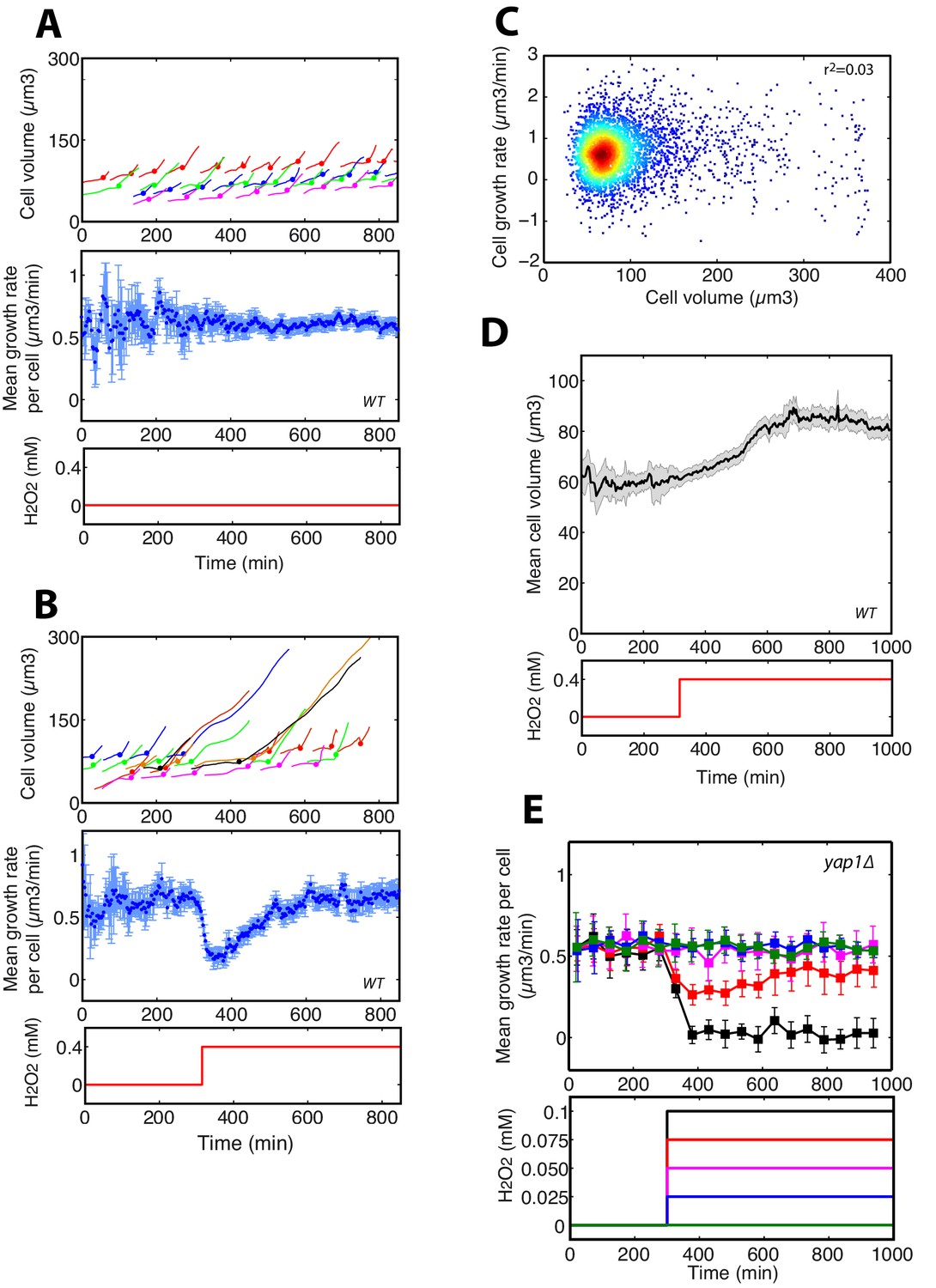
Principle of growth rate measurements.
(A) Growth rate measurements in the absence of stress. Top: cell volume of individual cells. Each color corresponds to a single cell followed over its successive divisions. The colored filled circle indicates a budding event. Middle: mean growth rate per cell as defined in Materials and methods. The error bars indicate the standard error of the mean (+/- SEM, N > 100 cells by the end of the experiment). Below: temporal profile of H2O2 concentration used during the experiment. (B) Same as (A), but following the switch from 0 to 0.4 mM H2O2 at t = 300 min. (C) Scatter plot showing the absence of correlation between cell growth rate and cell volume of individual cells. (D) Top: Evolution of mean (+/- SEM, N > 100 for most time points) cell size during the switch from 0 to 0.4 mM H2O2 at t = 300 min. Below: temporal profile of H2O2 concentration used during the experiment. (E) Similar experiment as in Figure 1E, but with the Δyap1 mutant.
Figure 2 with 3 supplements

DNA damage checkpoint and metabolic arrest during exposure to H2O2.
(A) Lineage of cells after addition of 0.5 mM H2O2 at t = 300 min. Each colored line corresponds to a single cell, and cell budding is indicated by the vertical black lines. The plot shows examples of cells with three distinct growth phenotypes, as indicated. (B) Quantification of the growth rate and division rate of the cellular phenotypes displayed in (A). Error bars are SEM. (C) Relative distribution (%) of cellular phenotypes as a function of H2O2 concentration added at t = 300 min. N = 100 for each concentration. (D) Top: Upregulation of cytoplasmic Rnr3-GFP expression at 300 min after addition of 0.4 mM H2O2. Bottom: Quantification of the Rnr3-GFP signal after addition of 0.4 mM H2O2. (E) Top: Upregulation of Ddc2-GFP expression at 300 min after addition of 0.4 mM H2O2. Bottom: Percentage of cells with durable Ddc2-GFP foci measured before and at 300 min after addition of 0.4 mM H2O2 for the cell phenotypes identified in (A). Error bars are 95% confidence intervals (CI). Two-proportions Z test. The whites bar represent 5 µm. See also Figure 2—figure supplement 1.
Figure 2—figure supplement 1

Lineage of cells following the exposure to 0.5 mM H2O2.
Top: Pedigree analysis of individual cells growing in the microfluidic during a typical H2O2 stress assay at 0.5 mM. Each colored line represents a single cell, and vertical black lines indicate cellular parentage. The vertical magenta line indicates the timing of switch to media containing H2O2. Each color corresponds to the phenotype acquired by the cells following the addition of stress. Bottom: same experiment as in the top panel but displaying the evolution of individual cell volume over time using the indicated color-coding.
Figure 2—figure supplement 2
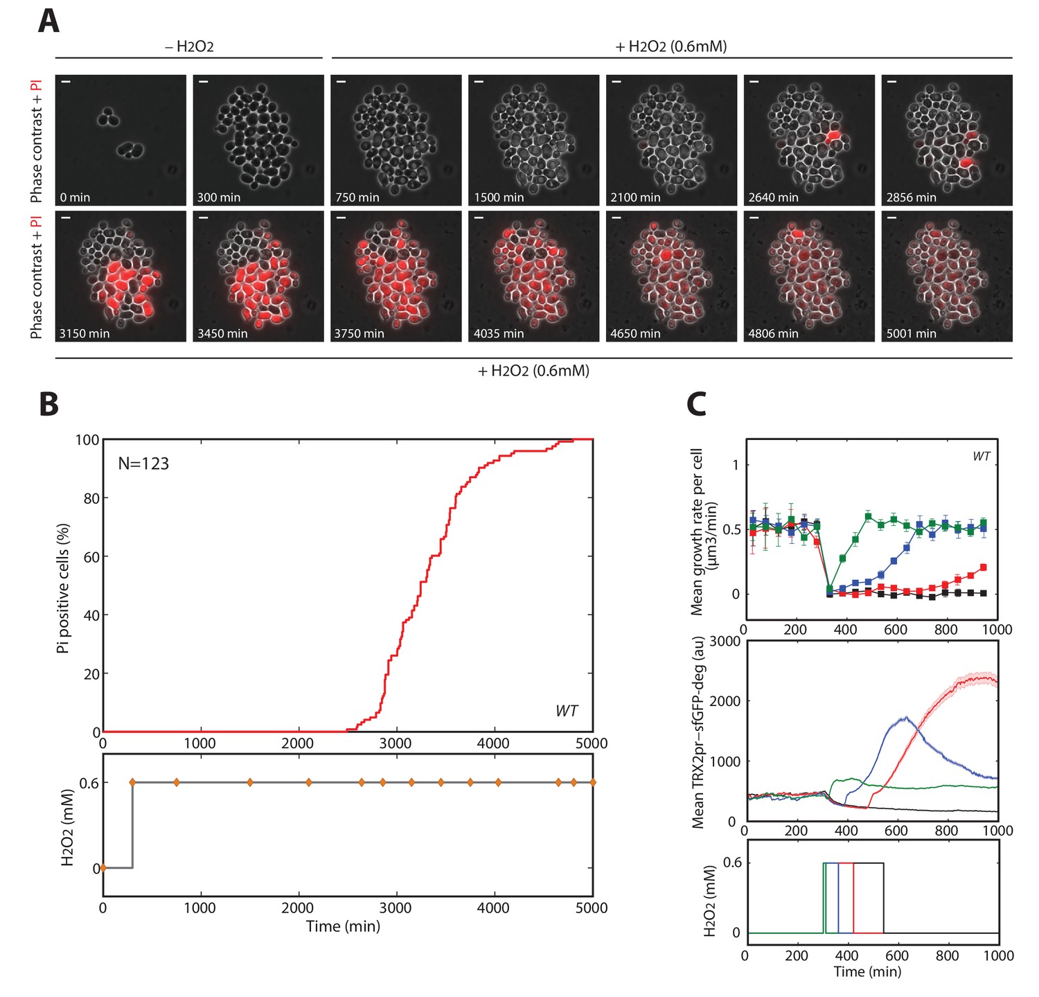
Cell death quantification during high (0.6 mM H2O2) step stress.
(A) Propidium iodide (PI)-based microfluidics essay detecting mortality in cells exposed to 0.6 mM H2O2 at t = 300 min. Red-colored (PI-positive) cells correspond to dead cells with loss of cell membrane integrity. The white bar represents 5 µm. (B) Top: Quantification of the PI incorporation by the cells displayed in (A) as a function of time. Bottom: Temporal profile of the H2O2 concentration. The orange filled circles correspond to the time points displayed in (A). (C) Reversibility of the growth arrest. Top: mean growth rate of cells exposed to 0.6 mM H2O2 for various durations, as indicated in the bottom panel. Middle: mean cellular expression of TRX2pr-GFP-deg; Bottom: schematics of the temporal profile of the pulse. Error bars are SEM (N > 100 for most time points).
Figure 2—figure supplement 3

Cell death markers for mild (0.4 mM H2O2) step stress.
(A) Cells exposed to 0.6 mM H2O2 (lethal stress) doesn’t induce Trx2-GFP and show bright vacuoles. Top: Quantification of Trx2-GFP level and the mean cellular intensity of the phase-contrast highest decile (note the increase in the intensity after stress addition revealing the presence of bright vacuoles, see Materials and methods). Middle: Temporal profile of the H2O2 concentration. Bottom: Phase-contrast and fluorescence images of individual cells right before (300 min) and 500 min after 0.6 mM H2O2 addition (801 min). (B) After addition of 0.4 mM H2O2, the fraction of cells with no growth recovery show low Trx2-GFP level and bright vacuoles. Top: Quantification of Trx2-GFP level and the mean cellular intensity of the phase-contrast highest decile. Middle: Temporal profile of the H2O2 concentration. Bottom: Phase-contrast and fluorescence images of individual cells 500 min after 0.4 mM H2O2 addition. The red contours show permanently arrested cells. (C) Summary of scoring of death markers in lethal (0.6 mM H2O2) and permissive (0.4 mM H2O2) step stress experiments. The white bars represent 5 µm.
Figure 3 with 2 supplements
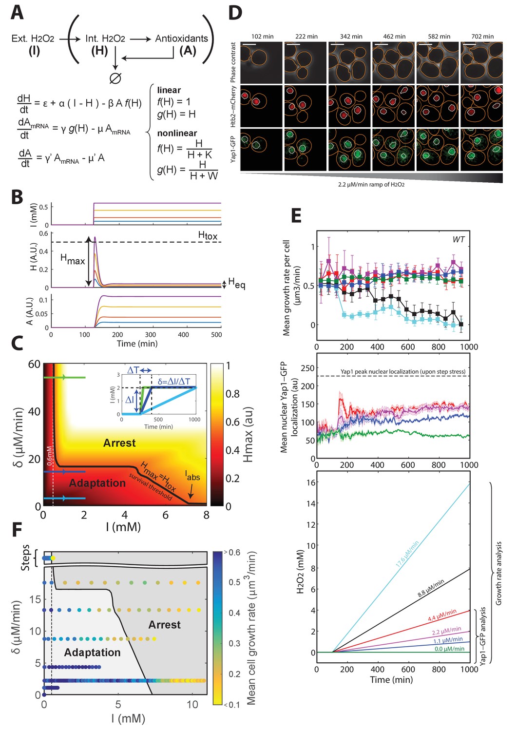
A negative feedback-based model to describe adaptation to H2O2.
(A) Schematic of the regulatory network involved in H2O2 scavenging: external H2O2 (represented by I), internal H2O2 (represented by H), and antioxidants (represented by A). A linear set of differential equations is used to describe the evolution of this system over time. (B) Response of the linear system described in panel (A) to sudden exposure to external H2O2 (step of amplitude I). Each colored line corresponds to a given concentration of H2O2. Heq is the steady-state internal H concentration, Hmax is the maximum H concentration reached during the transient regime. Htox is the threshold concentration beyond which growth/division is assumed to stop (obtained for I = 0.6 mM). (C) Phase diagram showing Hmax as a function of the amplitude of the step I and the rate of the H2O2 ramp δ = ΔI/ΔT. Inset shows a graphical representation of these parameters. The solid black line indicates the contour given when Hmax = Htox, assuming the general assumptions of the linear model described in panel A. (D) Sequence of phase-contrast and fluorescence images of individual cells at the indicated times after initiation (t = 100 min) of a linear ramped increase in H2O2 concentration at a rate δ of 2.2 μM/min. The red and green channels represent the Htb2-mCherry and Yap1-GFP signals, respectively. The white bars represent 5 µm. (E) Top: Mean growth rate per cell as a function of time after initiation (t = 100 min) of linear ramps in H2O2 concentration. The line colors correspond to the indicated ramp slopes in the bottom panel. Middle: Mean nuclear Yap1-GFP localization. Error bars and shaded regions are SEM, N > 100 for most time points. (F) Phase diagram recapitulating the mean growth rate of cells during adaptation to steps (Figure 1E) and linear ramps at various rates δ. The gray shading delimits the regions of adaptation and arrest, as expected from the linear feedback model. See also Figure 3—figure supplement 1 and Materials and methods.
Figure 3—figure supplement 1
Linear model: response to step, ramps, and training capabilities.
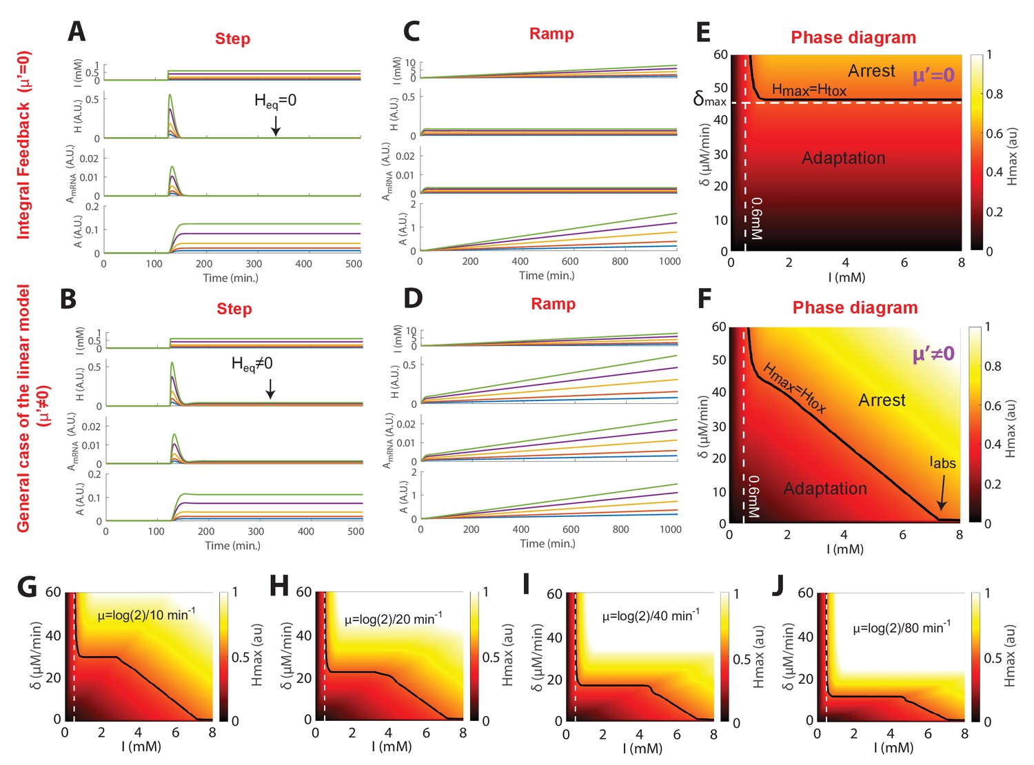
(A) Dynamics of model variables under the assumptions of a linear integral feedback model, when the system is submitted to a step concentration. Each color line represents the temporal evolution of the variables H, AmRNA and A following the switch to the indicated H2O2 concentration. Parameter values: ε = 0, α = 1 min−1, β = 5 min−1, γ = 0.53 min−1, γ’=0.01 min−1, μ= log(2)/2.5 min−1, μ’=0 min−1. (B) Similar as in (A), but in the general case of the linear model. Parameter values: ε = 0, α = 1 min−1, β = 5 min−1, γ = 0.53 min−1, γ’=0.01 min−1, μ= log(2)/2.5 min−1, μ’ = log(2)/100 min−1. (C) Similar as in (A), but during linear stress ramp. (D) Similar as in (B), but during linear stress ramp. (E) Phase diagram (similar to Figure 3C) for the case of an integral feedback model (μ’=0 min−1). (F) Similar as (E) for the general case of the linear model (μ’ = log(2)/100 min−1). (G–J) Phase diagram obtained with different values of mRNA decay rates (μ), as indicated, while keeping the value of Iabs = 7.3 mM.
Figure 3—figure supplement 2
Experimental setup to generate H2O2ramps and scoring of the permanent growth arrest phenotype.
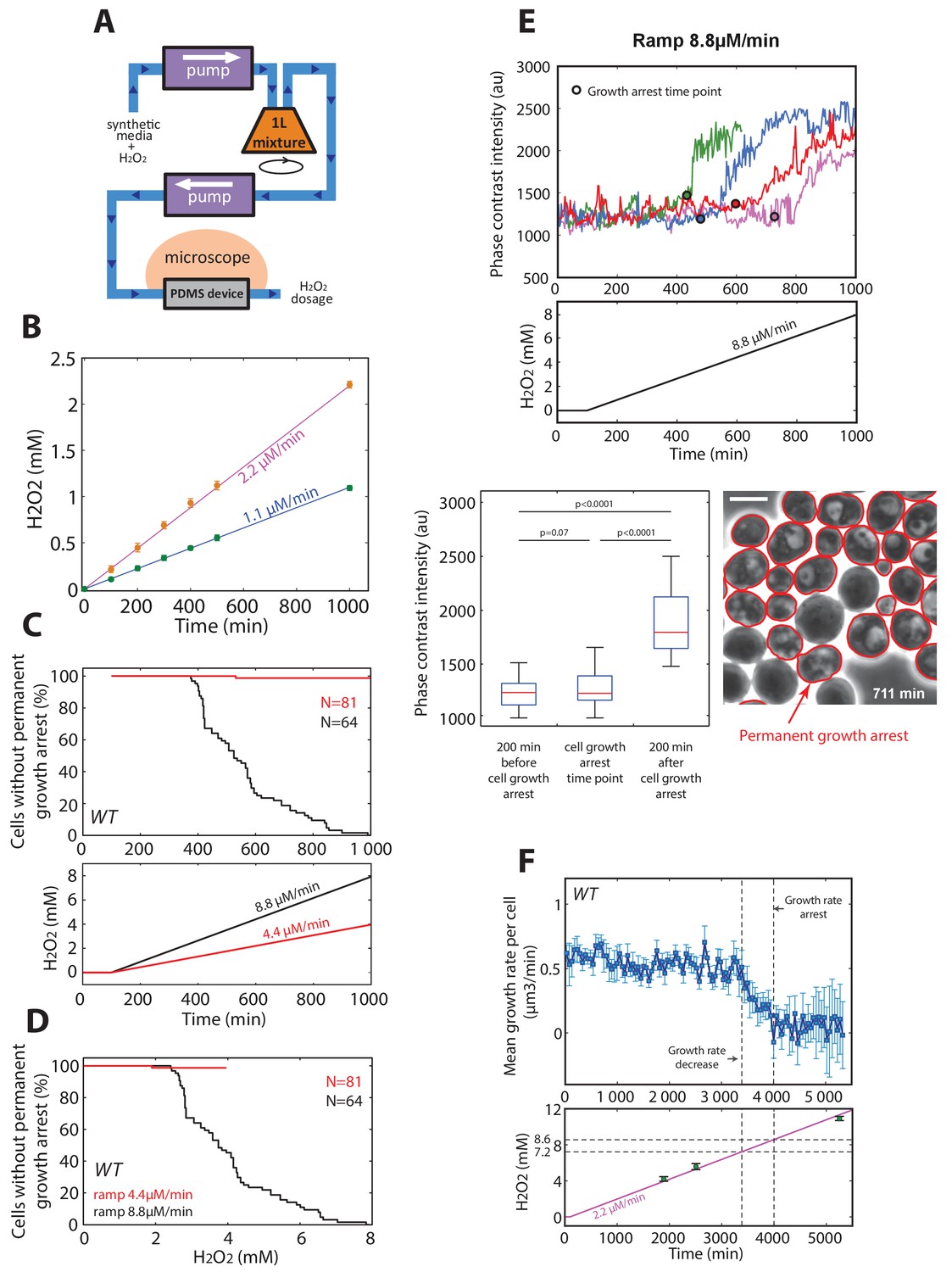
(A) Schematics of the setup used to generate linear ramps. (B) Dosage of H2O2 concentration during the ramp experiments performed using the setup described in (A). Each colored line corresponds to the expected ramp slope, whereas the actual H2O2 measurements are indicated as colored filled circles. Error bars are SEM, N = 3. (C) Top: Scoring of the fraction of cells able to grow as a function of time during ramped H2O2 stress. Only the cells present at the time of ramp initiation (t = 100 min) are scored. The red and black lines correspond to 4.4 µM/min and 8.8 µM/min H2O2 ramps, respectively. Cells are considered as not able to grow (permanent growth arrest) when their growth stops and does not recovers until the end of the experiment. Bottom: Temporal profile of the H2O2 concentration for both ramps. (D) Same experiment as (C), but the fraction of cells able to grow is represented as a function of the absolute H2O2 concentration. (E) Cells with permanent growth arrest during 8.8 µM/min H2O2 ramp show bright vacuoles. Top: the mean cellular intensity of the phase-contrast highest decile (see Materials and methods) is displayed for individual cells during the ramped stress. Middle: temporal profile of the H2O2 concentration. Bottom left: MatLab boxplot showing the quantification of the mean cellular intensity of the phase-contrast highest decile for the subpopulation of cells with permanent growth arrest during the ramp. The quantification is done at the moment of the cell growth arrest as well as 200 min before and after the growth arrest (N = 50, total of 64 cells but only 50 were scored because not all cells can be followed 200 min after growth arrest). Bottom right: phase-contrast image of cells 611 min after the initiation of 8.8 µM/min H2O2 ramp. The red contours show permanently arrested cells. Two-means Z test. The white bar corresponds to 5 µm. (F) Determination of hard limit H2O2 concentration allowing adaptation. Mean cell growth rate per cell as a function of time after initiation (t = 100 min) of linear ramps at a rate δ of 2.2 μM/min during 140 hr. Expected and measured (N = 6) H2O2 concentrations are displayed on the bottom panel. Error bars are SEM.
Figure 4 with 1 supplement
Mechanism of acquisition of tolerance to stress.
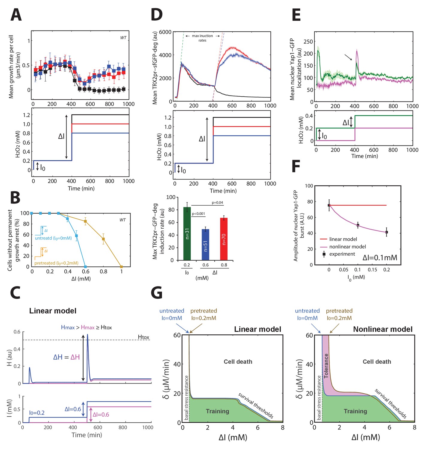
(A) Mean cell growth rate (top panel) of cells exposed to H2O2 steps of the magnitude indicated in the bottom panel at t = 400 min after a 0.2 mM pretreatment at t = 0 min. (B) Fraction of cells without permanent growth arrest at different concentrations of H2O2 in the presence (yellow) or absence (blue) of pretreatment. N = 100 for each concentration. (C) Response of the linear system to simple H2O2 step of amplitude ΔI = 0.6 mM for naive (magenta: I0 = 0 mM) or pretreated (bleu: I0 = 0.2 mM) cells. (D) Top: Mean cell transcriptional dynamics (top panel) of the TRX2 promoter (Trx2-sfGFP-degron) for the H2O2 treatments shown in the middle panel. Bottom: Quantification of the maximum transcription rate of the TRX2 promoter during the indicated steps. Two-means Z test. (E) Mean cell Yap1-GFP nuclear localization upon a 0.2 mM H2O2 step for cells with (green line) or without (magenta line) a 0.2 mM pretreatment, as indicated in the bottom panel. (F) Quantification of the amplitude of the burst in Yap1 nuclear localization during a 0.1 mM H2O2 challenge step. The lines indicate the fit of the linear (red) and nonlinear (magenta) models. (G) Numerical phase diagram indicating the region in which adaptation is permitted as a function of the overall stress magnitude ΔI and stress rate δ for the linear (left) and nonlinear (right) models. The solid black line indicates the contour given when Hmax = Htox (survival threshold) as in Figure 3C. The vertical dashed line represents the basal stress resistance, as observed in step experiments. The green color represents the region in which cells can be trained to resist higher stress levels through a slow ramping process. The magenta region highlights the shift in survival threshold obtained following a pretreatment according to the nonlinear model. A, D–F, error bars and shaded regions are SEM (N > 100 for most time points). B, error bars are 95% CI. See also Figure 4—figure supplement 1.
Figure 4—figure supplement 1
Acquisition of tolerance: comparison of the linear and nonlinear models.
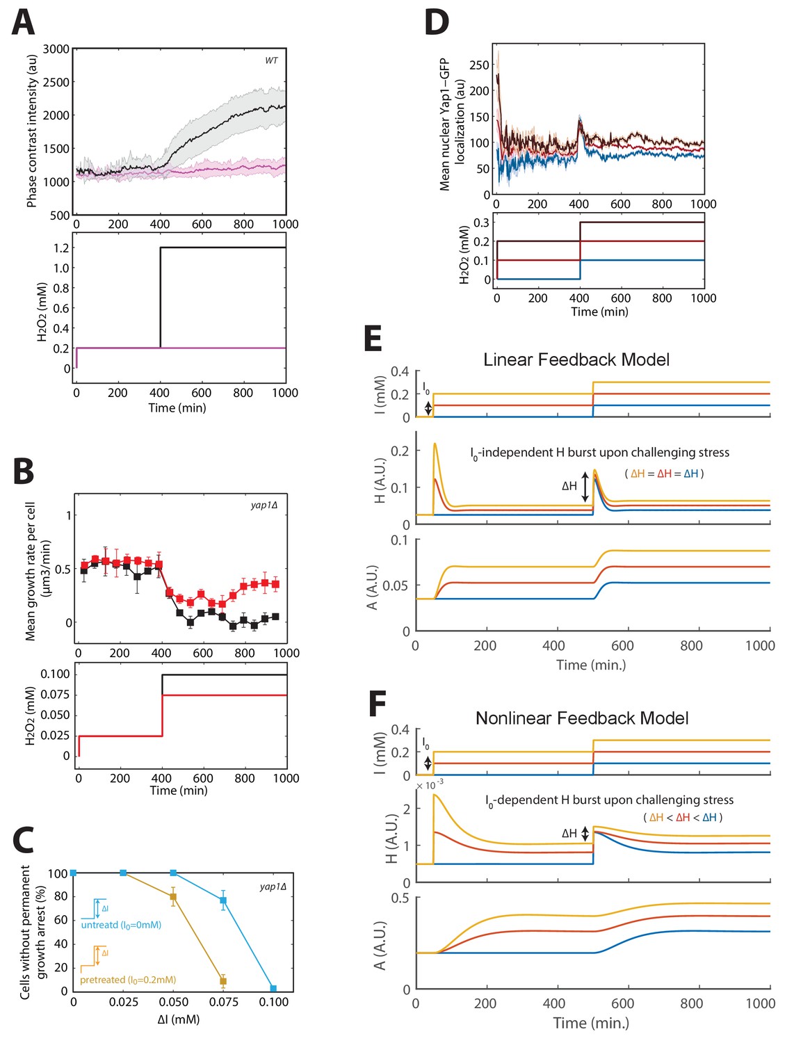
(A) The mean cellular intensity of the phase-contrast highest decile is quantified for a population of cells exposed to critical ΔI = 1 mM (black line) after pretreatment of I0 = 0.2 mM and for control population of cells only exposed to the pretreatment of I0 = 0.2 mM (magenta line). (B–C) Same as Figure 4A–B, but with the yap1Δ mutant. (D) Same as Figure 4E, but with various levels of H2O2 during pretreatment and with a challenging step of ΔI = 0.1 mM H2O2. The Yap1 maximal amplitudes from this graph are represented in Figure 4F. (E) Numerical simulation of the response of the H2O2 homeostatic machinery to a sequence of two consecutive stress steps of indicated amplitude (top), using the linear feedback model. The first step (I0) corresponds to the pre-treatment, while the second represents the challenging step (ΔI) described in Figure 4. Each colored line corresponds to a particular temporal profile of H2O2 concentration. H (Middle) and A (Bottom) are two variables of the model described in Figure 3 and Materials and methods. (F) Same as (E), but for the nonlinear feedback model. (A,B,D) Error bars and shaded regions are SEM (N > 100 for most time points). (C) error bars are 95% CI.
Figure 5 with 1 supplement
Genetic determinants of adaptation to ramped increases in H2O2.
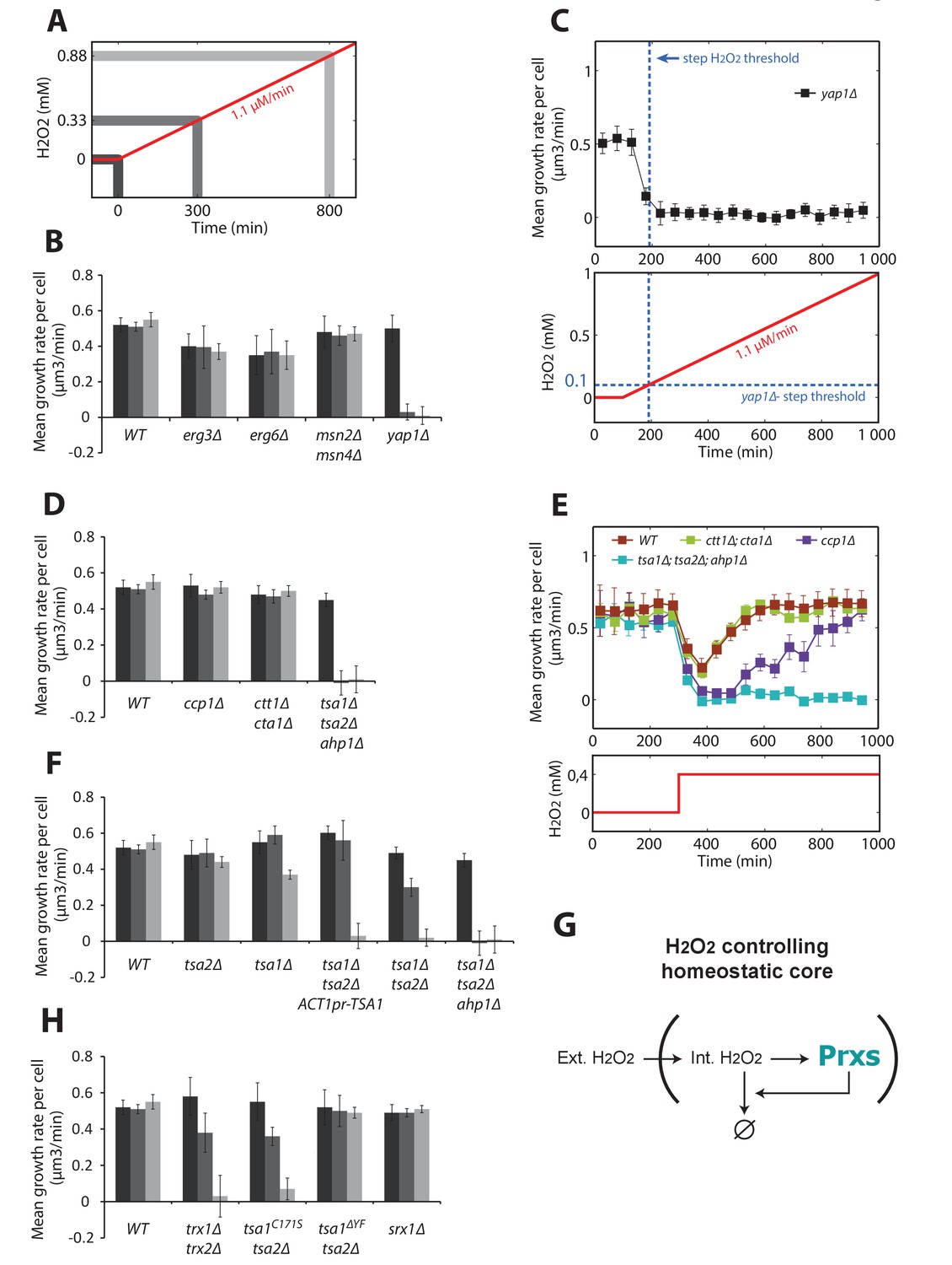
Quantification of mean growth rate upon exposure to a linear ramp (δ = 1.1 μM/min) starting at t = 100 min in various genotypes. (A) Illustration of the H2O2 ramp experiment indicating the timing of the measurements. (B) Stress response and membrane permeability mutants. (C) Details of the ramp experiment in the Δyap1 mutant. The dashed blue lines indicate the adaptation threshold obtained in step experiments (Figure 1G). (D) Yap1 effectors mutants. (E) Step experiment performed with Yap1 effectors mutants exposed to 0.4 mM H2O2. (F) Prxs mutants. (G) Schematic of a negative feedback control showing the essential role of Prxs in the H2O2 homeostasis. (H) Mutants affecting the peroxidatic cycle of Prxs. Error bars are SEM (N > 100). See also Figure 5—figure supplement 1.
Figure 5—figure supplement 1

Quantification of Tsa1 expression from the ACT1 promoter.
(A) Phase and GFP fluorescence image samples of cells carrying a Tsa1-GFP fusion (top) or an ACT1pr-TSA1-GFP fusion (bottom). (B) Quantification of mean cell cytoplasmic fluorescence for strains described in (A) Error bars are SEM (N > 100).
Figure 6 with 1 supplement
Tsa1 scaling properties.
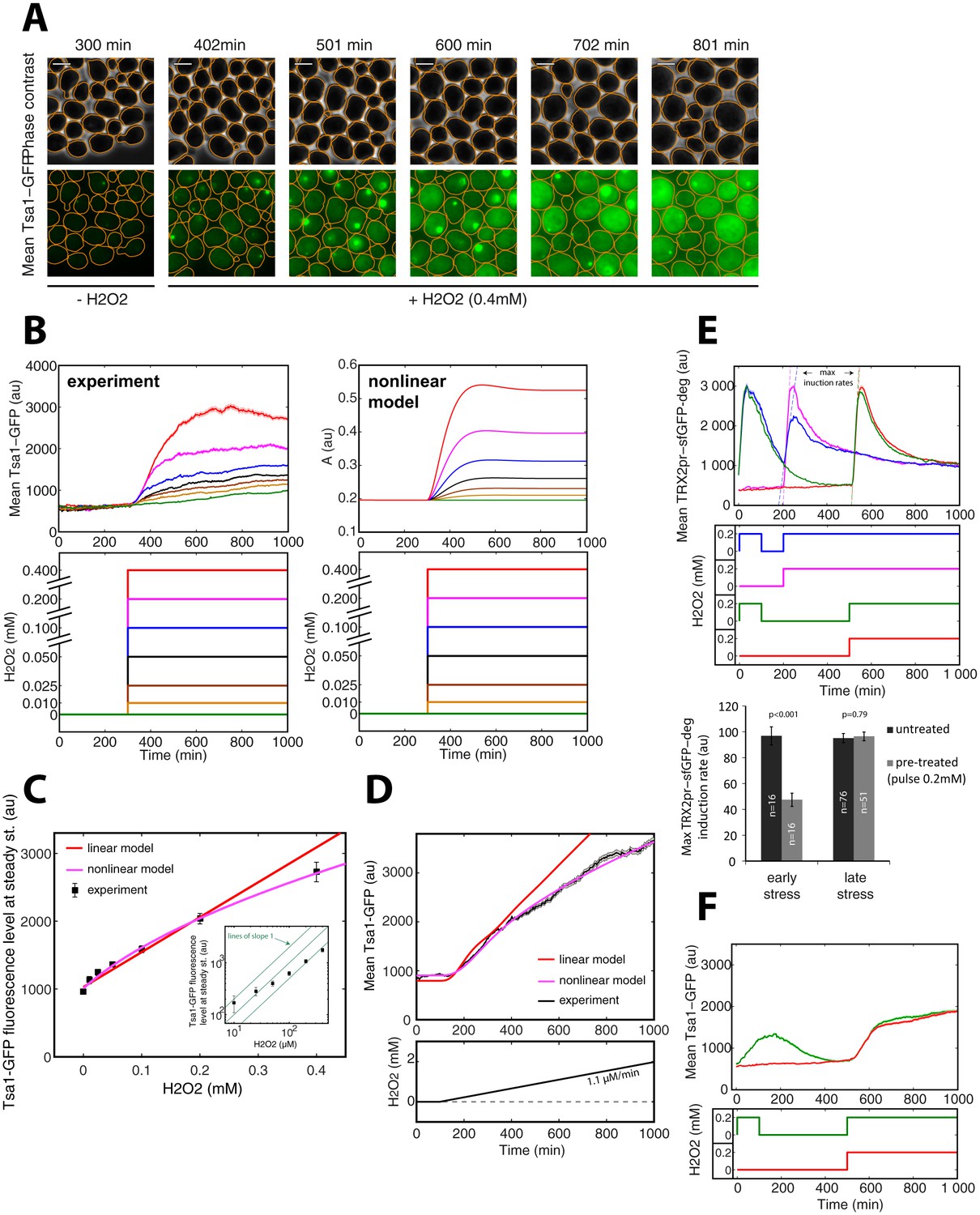
(A) Sequence of phase-contrast and fluorescence images of individual cells at the indicated times after initiation (t = 300 min) of a 0.4 mM step in H2O2 concentration. The green channel represents the Tsa1-GFP signal. The white bars represent 5 µm. (B) Left: Mean cell expression (top) of Tsa1-GFP following the H2O2 steps indicated in the bottom panel. Right: Dynamics of antioxidant level with increasing stress, as expected from the nonlinear model. (C) Quantification of mean cell expression of Tsa1-GFP at steady state as a function of H2O2 concentration (from experiments in (B)). Colored lines indicate the fit of the linear (red) and nonlinear (magenta) models. Inset: log-log representation of Tsa1-GFP level with H2O2 level. Green lines indicate lines of slope one on a log-log scale, to emphasize the nonlinearity of Tsa1-GFP expression. (D) Mean Tsa1-GFP expression (top) during a ramp experiment, as indicated in the bottom panel. Colored lines indicate the fit of the linear (red) and nonlinear (magenta) models. (E) Top: Mean cellular transcription of the TRX2 promoter for cells exposed to the temporal H2O2 profiles described in the middle panel (with corresponding color coding). Bottom: Quantification of maximal transcriptional output during a step experiment performed at t = 200 min (early stress) or 500 min (late stress) with or without pretreatment. Student’s t-test. (F) Mean cellular expression of Tsa1-GFP for cells exposed to the temporal H2O2 profiles described in the bottom panel. Error bars and shaded regions are SEM (B,D-F: N > 100 for most time points, C: N > 100).
Figure 6—figure supplement 1
Analysis of the TSA1 promoter activity during H2O2stress.
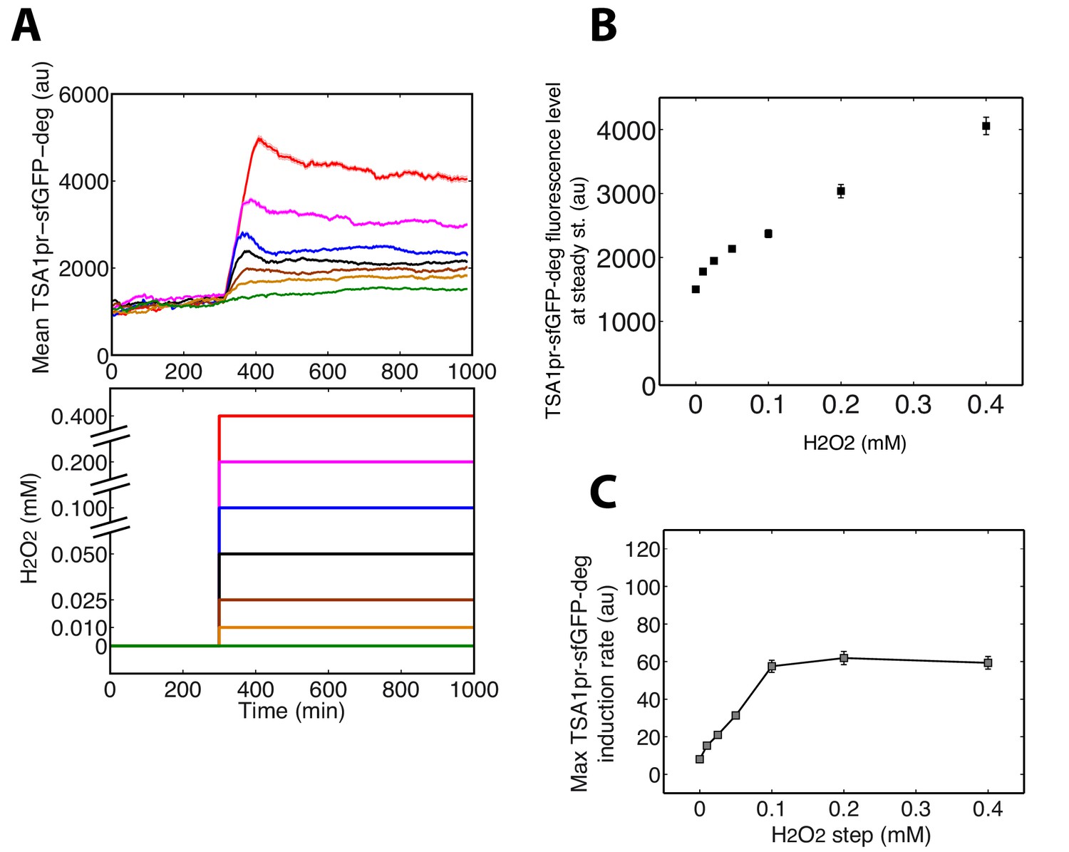
(A) Dynamics of the mean transcriptional response of TSA1 promoter (TSA1pr-sfGFP-deg) in step experiments at indicated H2O2 concentrations. (B) Quantification of mean cell expression of TSA1pr-sfGFP-deg at steady state as a function of H2O2 concentration (from experiments in (A)). (C) Quantification of the maximal transcription rate of TSA1 promoter during a step experiment, as a function of the amplitude of the stress. The transcription rate was calculated by fitting a line over a 18-min time window to the data reported in (A) and by determining the maximal slope. Error bars and shaded regions are SEM (A) N > 100 for most time points, (B and C) N > 100.
Figure 7
Hormetic effect of H2O2 on replicative longevity.
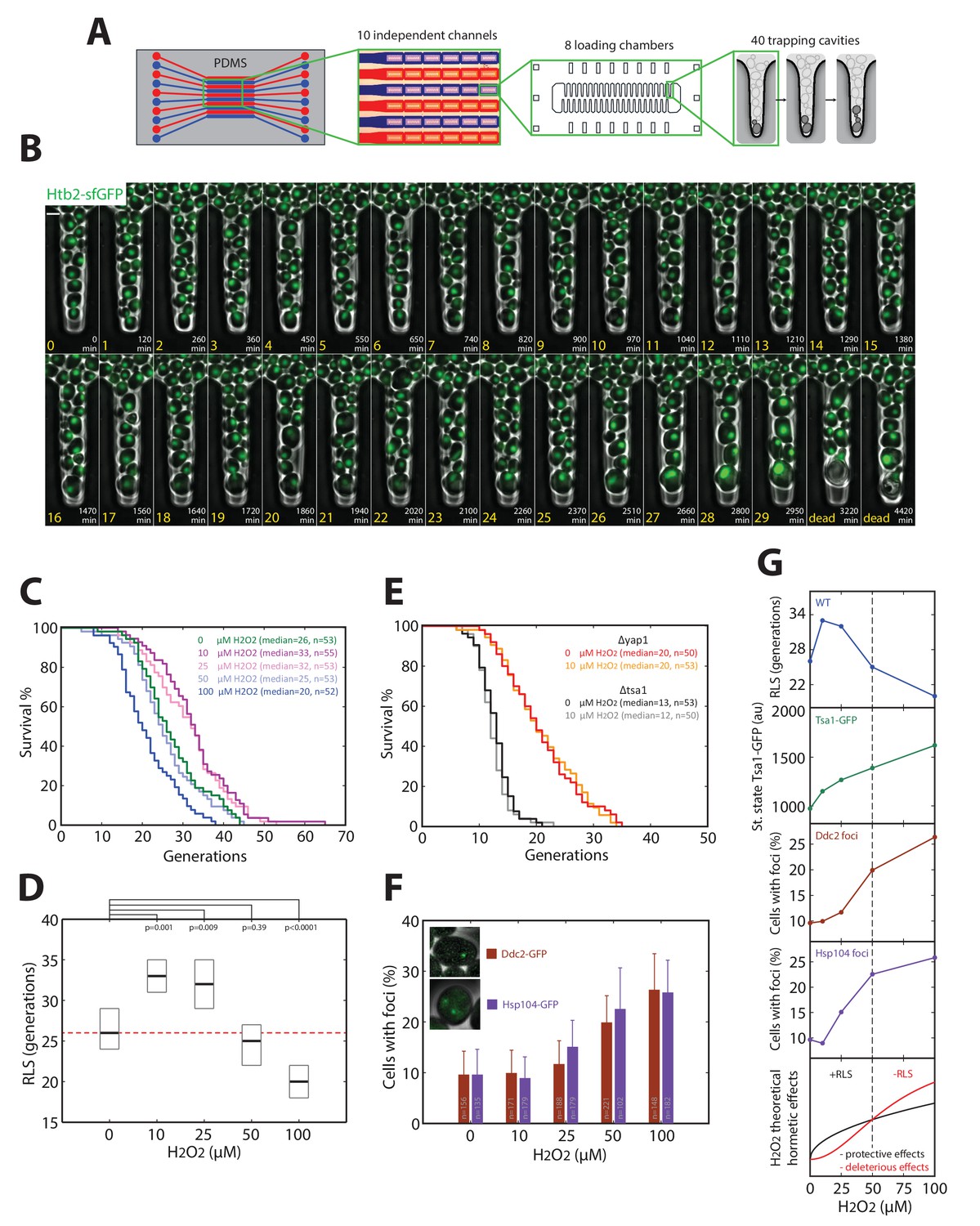
(A) Sketch of the microfluidic device used for replicative aging experiments. (B) Sequence of overlaid phase-contrast and fluorescence images (Htb2-sfGFP, used as a nuclear marker to score cell division) of mother cells growing in individual cavities. Numbers indicate the timing (white) and number of cell divisions (yellow) for the mother cell at the tip of the cavity. (C) Survival curves for wild-type cells growing in media containing H2O2 at the indicated concentrations. (D) RLS as a function of H2O2 concentration. Box represents median and 95% CI. U test. Red line shows the median RLS for 0 mM H2O2. (E) Survival curves of Δyap1 and Δtsa1 mutants in the presence or absence of 10 μM H2O2. (F) Frequency of specific fluorescence foci (Ddc2-GFP, Hsp104-GFP) as a function of H2O2 concentration. Error bars are 95% CI. (G) (Top to bottom) Recapitulation of measurements of RLS (blue), Tsa1-GFP steady-state upregulation (green), and frequency of damage (DDC2 foci in brown, Hsp104 foci in purple). Bottom: Conceptual sketch showing the contributions of protective (black) and deleterious (red) effects of H2O2 on RLS.
Videos
Video 1
Growth rate monitoring upon H2O2 stress (refers to Figure 1)
Movie showing a time-lapse experiment where cells are exposed to sudden step stress of 0.4 mM H2O2 at t = 300 min. Left: phase contrast, right: growth rate evolution graph. The white bar represents 5 µm.
Video 2
Yap1 nuclear relocation upon H2O2 stress (refers to Figure 1)
Movie showing the nuclear enrichment of Yap1 in cells exposed to 0.4 mM H2O2 at t = 300 min. Left: Phase contrast and mCherry (Htb2-mCherry) channels. Right: GFP (Yap1-GFP) channel. The white bar represents 5 µm.
Video 3
Cell metabolic arrest at high H2O2 dose (refers to Figure 1)
Movie showing a permanent cell growth arrest in cells exposed to 0.6 mM H2O2. Left: phase contrast, right: growth rate evolution graph. The white bar represents 5 µm.
Video 4
Phenotypic variability upon H2O2 stress (refers to Figure 2)
Movie showing different cell fates in cells exposed to 0.5 mM H2O2 at t = 300 min. Blue cell contours: Adapted cells; Yellow cell contours: Prolonged cell cycle arrest; Red contours: Permanent growth arrest. The white bar represents 5 µm.
Video 5
Cell mortality at high H2O2 step stress (refers to Figure 2—figure supplement 2)
Movie showing the incorporation of PI in cells exposed to 0.6 mM H2O2 at t = 300 min. The white bar represents 5 µm.
Video 6
Replicative lifespan monitoring (refers to Figure 7)
Movie showing the entire lifespan of a cell from birth to death in a cavity of PDMS device. The white bar represents 5µm.
Additional files
-
Supplementary file 1
List of all strains used in this study.
Table listing the strains used in this study as well as additional information about the genotypes and the origins of the strains.
- https://doi.org/10.7554/eLife.23971.026
Download links
A two-part list of links to download the article, or parts of the article, in various formats.
Downloads (link to download the article as PDF)
Open citations (links to open the citations from this article in various online reference manager services)
Cite this article (links to download the citations from this article in formats compatible with various reference manager tools)
Nonlinear feedback drives homeostatic plasticity in H2O2 stress response
eLife 6:e23971.
https://doi.org/10.7554/eLife.23971


