Minimal-assumption inference from population-genomic data
Figures
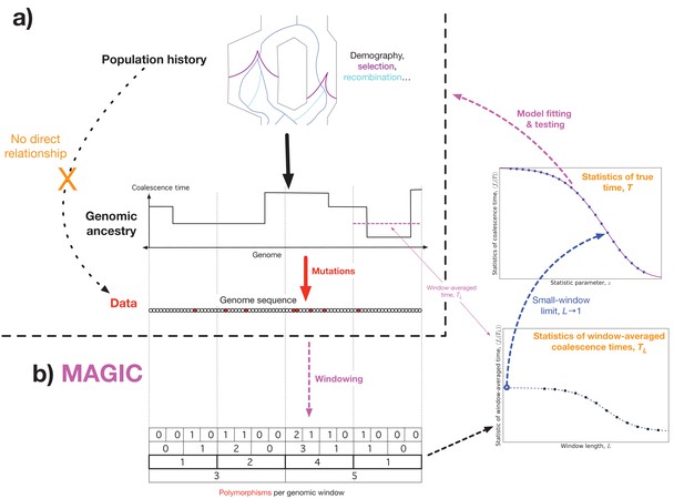
Outline of approach.
(a) Concept: we would like to infer the history of the population (top) from the sequence data (bottom), but the causal connection between the two is entirely mediated by the coalescent history of the sample (middle). This suggests that it should be possible to extract much of the coalescent information from the data without making strong assumptions about the population dynamics. (b) Schematic algorithm: MAGIC first splits the sample into small windows and counts the polymorphisms within each window, then progressively merges pairs of adjacent windows together (bottom left). For each window length , the histogram of window diversity is used to estimate parameters of the distribution of the window-averaged coalescence time (bottom right). Taking the limit of these as goes to 1 gives the parameters of the distribution of the true coalescence time (top right), which are then used to fit and test models for the underlying dynamics.
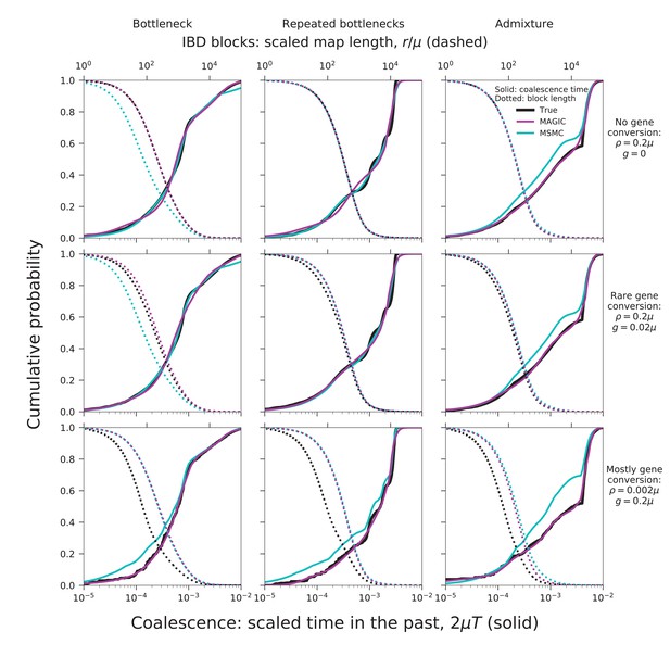
MAGIC accurately infers the distribution of coalescence times (solid curves) and lengths of blocks of identity-by-descent (IBD, dotted curves) for pairwise data simulated with ms under several demographic scenarios (Figure 9): a single bottleneck (left column), repeated expansions and contractions (middle), and recent admixture of two diverged populations (right).
The coalescence time plots show the cumulative distribution, while the IBD block-length plots show the survival function. When crossovers are frequent and gene conversion is rare (top two rows), MAGIC and MSMC are comparably accurate for coalescence times. MAGIC very accurately infers the IBD block length distribution, while MSMC sometimes is inaccurate (e.g., ‘Bottleneck’ scenario), but otherwise produces a curve nearly indistinguishable from MAGIC’s. For frequent gene conversion and rare crossovers (bottom row), the details of the gene conversion process have a strong effect on the IBD block lengths, and neither method can infer their distribution, but MAGIC can still infer the coalescence times. All simulations are of a genome consisting of independent chromosomes, each base pairs long, with per-base mutation rate and present population size such that . Recombination is via crossovers occurring at rate per base, and via gene conversion being initiated at rate per base with mean tract length . See Materials and methods for values of other simulation parameters.
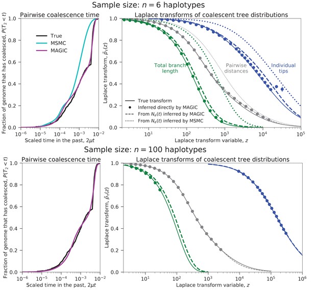
Coalescence time distributions and their Laplace transforms for a simulated population with ancestral structure, as inferred from samples of intermediate and large size.
Top row: sample size haplotypes. MAGIC accurately estimates the distribution of the pairwise coalescence time (top left), and the Laplace transforms of the distributions of the total branch length and the lengths of the tips of the branches (top right, green and blue, respectively). The gap between the estimated Laplace transforms (circles) and that obtained by simulating the estimated from the pairwise coalescence time distribution (green and blue dashed curves) suggests that the model is inaccurate. The pairwise Laplace transforms are shown in gray for comparison. MSMC’s inferences are less accurate. Bottom row: sample size haplotypes (too large for MSMC). The gap remains between the estimated Laplace transform of the total branch length distribution and that derived from the pairwise , showing that the coalescent process cannot be described by a single . However, the tip length distribution matches that predicted from the pairwise comparisons, showing that the model has predictive power for recent times.
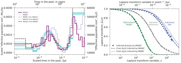
Inferred evolutionary history of Yoruban individuals.
Left: Inferred ‘effective population size’ for the nine unrelated Yoruban individuals from the 69 Genomes data set (Drmanac et al., 2010). MAGIC’s inference from the full sample is similar to MSMC’s inference from each individual, differing mostly in the distant past where there is limited data. Dotted lines show inference from samples simulated under the inferred ’s, indicating that MAGIC’s inference in the distant past is likely to be more accurate than MSMC’s, but that its inference of the fine-scale structure in is unreliable. Right: Laplace transforms of the distributions of different coalescence times for the same sample. The pairwise coalescence time (corresponding to in the left plot) is in gray, while the total branch length is in green and the distribution of tip lengths is in blue. Points show the values inferred directly by MAGIC, while solid and dashed curves show the results of simulations based on the curves inferred by MAGIC and MSMC, respectively. The pairwise accurately describes the distribution of total branch lengths, but overestimates the tip length Laplace transform (i.e., underestimates the tip lengths). MAGIC’s overestimate roughly corresponds to a underestimate of the median tip length, while MSMC’s corresponds to a underestimate, indicating that both underestimate recent from pairwise data.
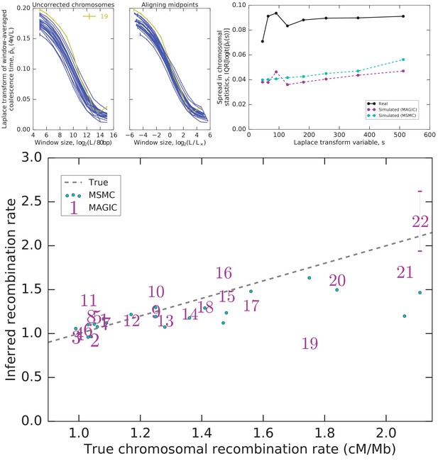
Integrating diversity patterns across length scales allows to compare recombination rates among chromosomes and to test whether the observed patterns can be explained by a single shared demographic history.
Top left: One value of the Laplace transform of the window-averaged coalescence time distribution as a function of window size for each autosome. The curves for most autosomes appear similar, but shifted both vertically and horizontally. Top center: Much inter-autosomal variation can be explained by variation in recombination rates: the curves are similar under a rescaling of window lengths (a horizontal shift such that the midpoints of the curves align), except for chromosome 19 (yellow), which appears to have a different pattern of coalescence. Top right: There is substantial variation in the asymptotes that cannot be explained by variation in recombination rates, and is more than expected from intrinsic coalescent stochasticity. Plot shows the interquartile range (IQR) of the Laplace transform of the coalescence time distribution across chromosomes for the actual data as well as simulations of the pairwise coalescent histories inferred by MAGIC and MSMC (Figure 4). (Note that IQR, unlike variance, is insensitive to outliers.) Bottom: The rescaling of window sizes needed to align the different autosomes gives an estimate of their relative recombination rates which is very close to the values obtained by Kong et al. (2002) (‘True’). For chromosomes other than 22, the inferred error bars are smaller than the size of the markers.
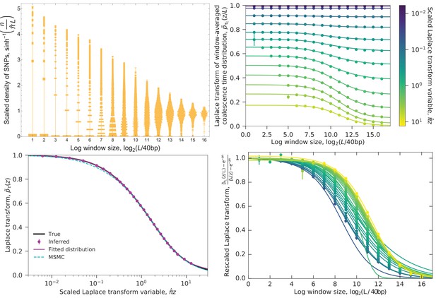
Example of converting the distribution of SNPs to the coalescence time distribution.
Data are from the simulated ‘bottleneck’ demography (Figure 2 and Figure 9, left columns). Top left: Distribution of SNP densities across windows of different lengths, normalized by the heterozygosity . The width of a bar represents the fraction of windows with a given SNP density. The densities are shown on an arcsinh scale (approximately logarithmic for large values but linear for small values). At short lengths, the distribution is concentrated at zero, while at long lengths it is bunched near the mean, with the best spread in between. Top right: The Laplace transform of the window-averaged coalescence time distribution as a function of window length and Laplace transform variable . Points show the estimates derived from the SNP density distribution (using Equation 3, with error bars given by Equation 4), curves are sigmoid fits (Equation 5). For small (long times), small windows can be used to estimate the left asymptote , while for large (short times), the estimates from small windows diverge (missing points with )) and longer windows need to be used. Typical coalescence times correspond to (blue-green). Bottom left: Laplace transform of the coalescence time distribution. Points are the left asymptotes of the curves in the top right panel. Black curve shows the true transform, magenta curve shows MAGIC’s fitted distributions (the gamma mixture and piecewise exponential forms give indistinguishable curves), cyan curve shows the Laplace transform of MSMC’s estimated coalescence time distribution. All the curves are close, but differ slightly for very large , corresponding to very recent times, with MSMC also differing for small (ancient times). Bottom right: Same as top right, rescaled to show that as increases, longer windows are sufficient to accurately estimate . But the increase in the minimum sufficient window length is slower than the increase in the minimum length for which can be accurately estimated (top right, leftmost points), putting a limit on the maximum for can be estimated (bottom left, rightmost point).
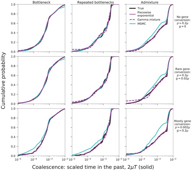
Comparison of the functional forms for the coalescence time distribution.
The inferred piecewise exponential (solid magenta) and gamma mixture (dashed purple) distributions are very similar, but where they differ, the piecewise exponential form is closer to the true distribution (black). Simulations are the same as shown in Figure 2. The two forms’ predicted block-length distributions (dotted curves in Figure 2 are indistinguishable.
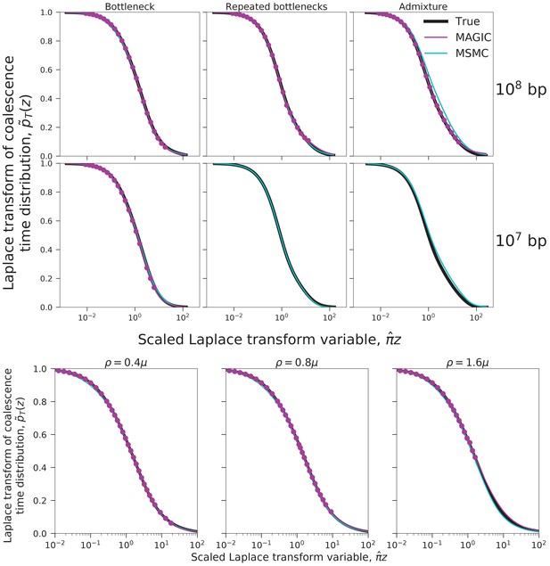
Limits on inferring the Laplace transform of simulated pairwise coalescence distributions.
Symbols and colors are as in the bottom left panel of Figure 6. Top: MAGIC can usually accurately infer the Laplace transform from sequenced bases (top row), but often fails when the data is limited to bases (bottom row, right two panels). Even under limited data, the inferences that it does manage to make remain accurate (bottom row, left panel). Other simulation parameters are as in the top row of Figure 2. Bottom: MAGIC can infer most of the Laplace transform when the crossover rate, , is less than the mutation rate, (left two panels), but for (right panel), it becomes limited to large . Simulation parameters are as in the top left panel of Figure 2, with increased.
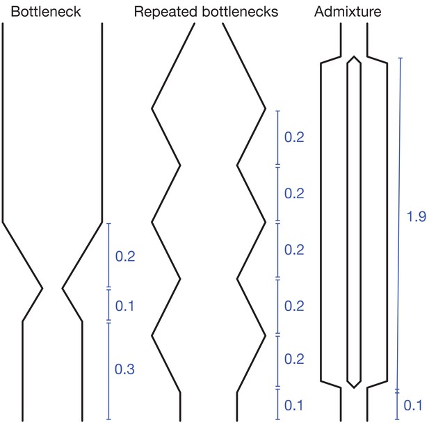
Demographic scenarios simulated.
All time intervals are in units of . In the ‘bottleneck’ and ‘repeated bottlenecks’ scenarios, the population grows and shrinks exponentially at rate .


