Physical limits of flow sensing in the left-right organizer
- Institut de Génétique et de Biologie Moléculaire et Cellulaire, France
- Centre National de la Recherche Scientifique, France
- Institut National de la Santé et de la Recherche Médicale, France
- Université de Strasbourg, France
- J. Stefan Institute, Slovenia
- Max-Planck-Institute for the Physics of Complex Systems, Germany
- Ecole Polytechnique, Centre National de la Recherche Scientifique (UMR7645), Institut National de la Santé et de la Recherche Médicale (U1182) and Paris Saclay University, France
Figures
Figure 1 with 1 supplement
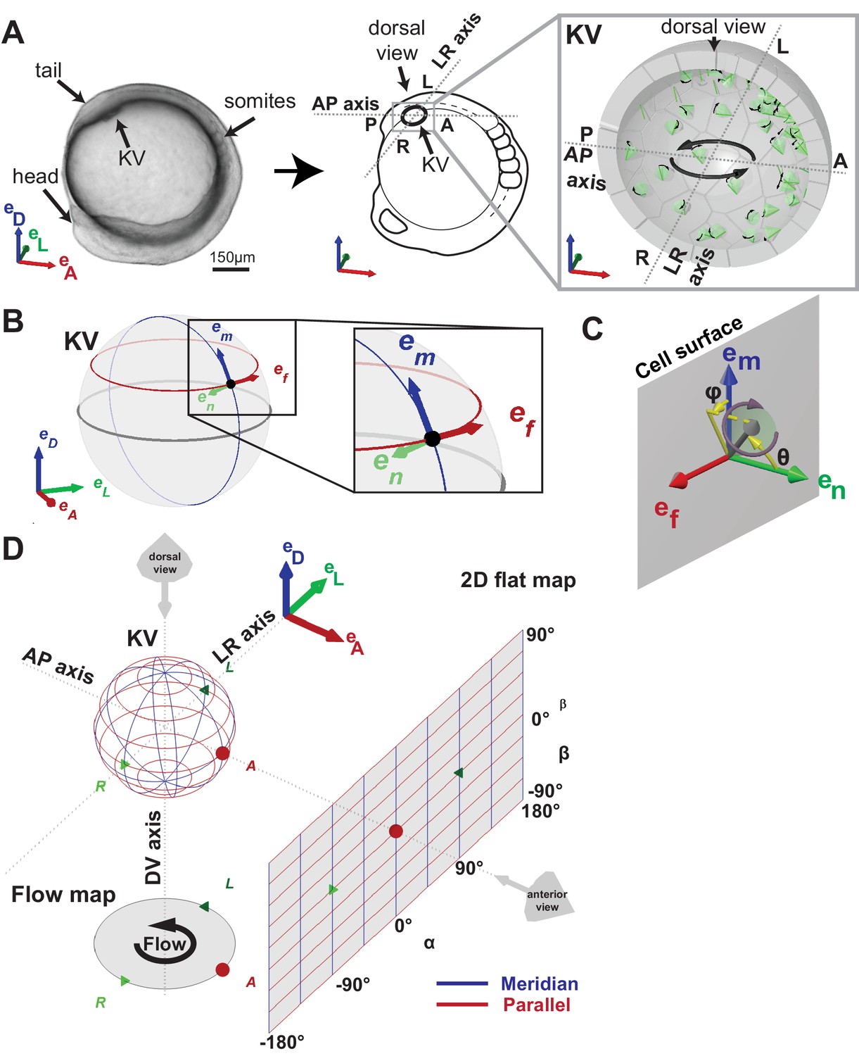
Definition of coordinate systems of the Kupffer’s vesicle (KV).
(A) Side view of a zebrafish embryo at 5-somite stage (left panel) and its schematic drawing (middle panel), highlighting the KV localization (grey box). The zoom-up box (right panel) shows the schematic transverse section of the KV, depicting the cilia (in green), their rotational orientation (black curved arrows) and the directional flow (thick black arrows). (B) em, en, ef are the local basis on the ellipsoid, which are used to define cilia orientation. The vector em is aligned along a meridian (blue) from the ventral to the dorsal pole; ef follows a parallel (red) in the direction of the typical directional flow within the vesicle; en is the vector normal to the KV surface and pointing towards the center of the vesicle (green). (C) Cilia 3D orientation is quantified by two angles: θ (tilt angle from the surface normal en) and φ (angle between the surface projection of the cilia vector and the meridional direction). (D) 2D flat map representation of the KV surface with coordinates α and β. The origin is set in the anterior pole. The embryonic body plan directions are marked as A (anterior), P (posterior), L (left), R (right), D (dorsal) and V (ventral). The body plan reference frame is defined as vectors eD, eL, eA.
Figure 1—figure supplement 1
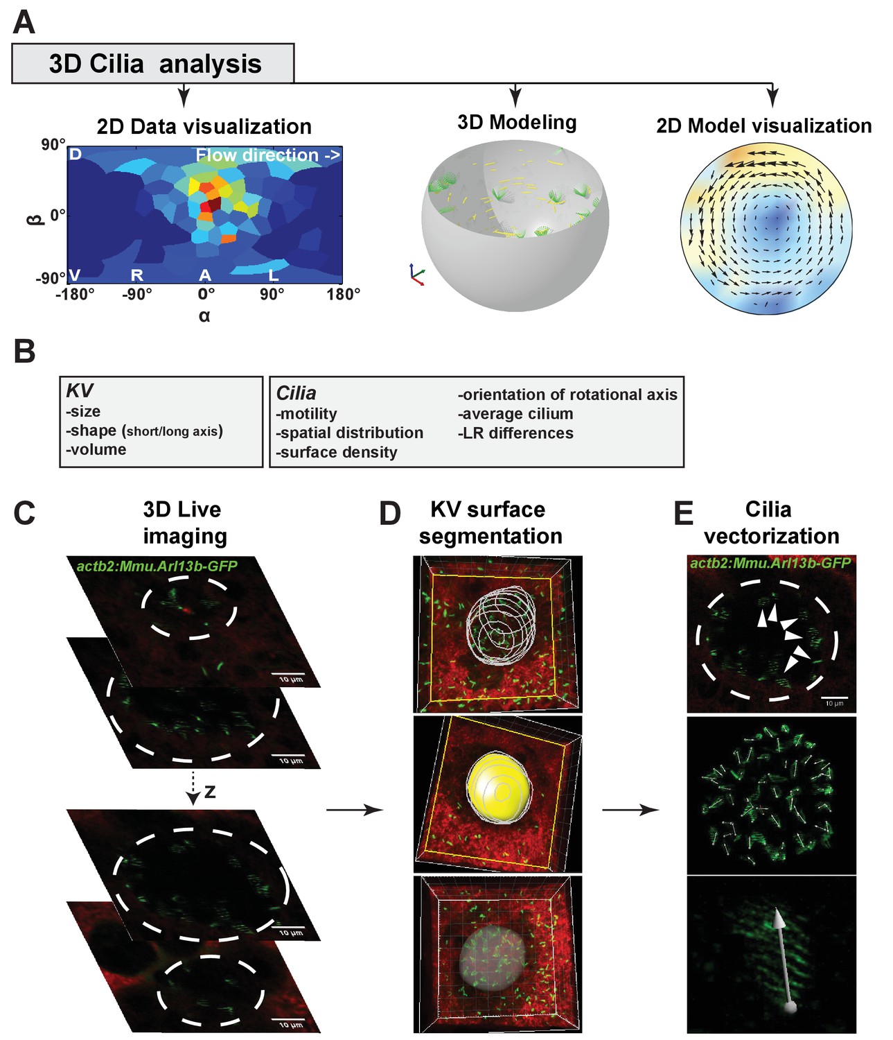
Multiscale analysis from individual cilia to 3D modeling of the Kupffer’s vesicle (KV).
(A) 3D-CiliaMap workflow pipeline: 3D live imaging with cilia analysis, followed by 2D visualization of cilia maps, 3D flow calculation based on live datasets, and flow visualization. (B) List of the KV and cilia features extracted using 3D-CiliaMap. (C–E) Successive steps forming the 3D-CiliaMap workflow from 3D live imaging to cilia vectorization (see also Video 1): (C) 3D live imaging of the total volume of the KV, using Tg (actb2:Mmu.Arl13b-GFP) (Borovina et al., 2010) embryos soaked for 60 min in Bodipy TR (Molecular Probe) - dashed white lines underline the KV. (D) Using Imaris (Bitplane Inc.), the KV surface is manually segmented to reveal only the cilia belonging to the surface of the KV cells. (E) Slow acquisition speed with standard laser scanning microscopy allows detecting the cilia orientation in the KV using the Tg (actb2:Mmu.Arl13b-GFP) line: dashed white lines underline the KV (upper panel); dorsal view of the whole vesicle showing the vectors obtained from the GFP signal (middle panel); high magnification of a cilium with a vector corresponding to its rotational axis orientation (bottom panel).
Figure 2
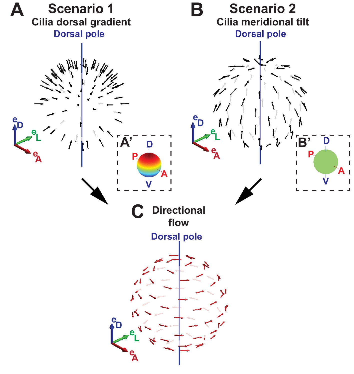
Two scenarios for the origin of directional flow.
(A) Scenario 1 – dorsal gradient: cilia unit vectors (black) are orthogonal to the surface, but the cilia density increases from the ventral to the dorsal pole. (B) Scenario 2 – meridional tilt: cilia are tilted along the meridians towards the dorsal pole. The insets in (A’–B’) show the density maps on the sphere: a linear dorsal gradient for scenario 1 (A’) and a uniform density for scenario 2 (B’) (color map from blue to red representing low to high cilia density). (C) Both scenarios can theoretically account for the directional flow (red arrows) rotating about the dorsoventral axis observed experimentally. See Figure 1 for the definition of the body plan reference frame and coordinates systems.
Figure 3
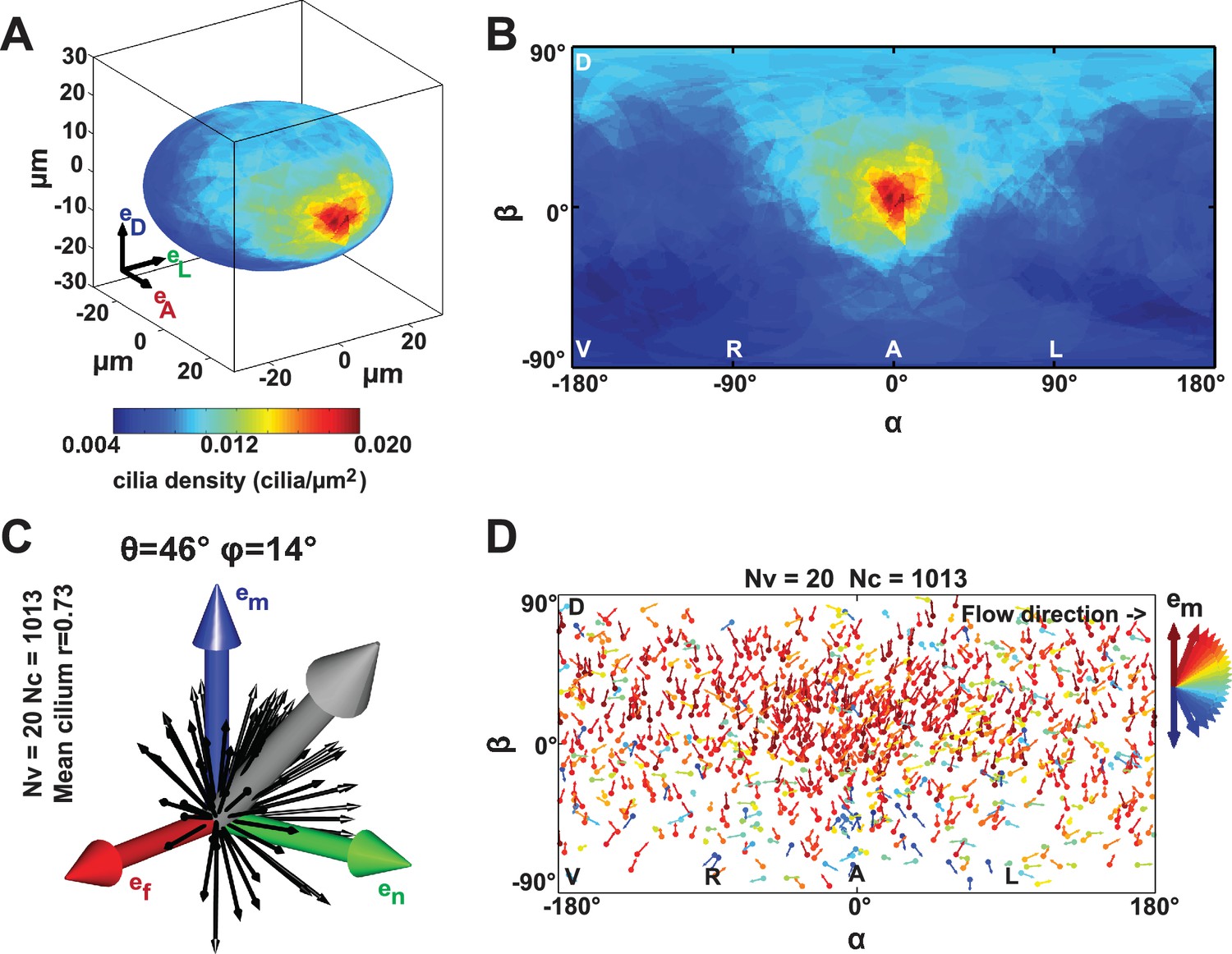
Anterior gradient of cilia density and cilia meridional tilt in the Kupffer’s vesicle (KV) at 8- to 14-somite stage (SS).
(A–B) Averaged cilia density obtained from 20 vesicles represented on a 3D KV map (A) or on a 2D flat map (B) revealing a steep density gradient along the anteroposterior (AP) axis and the resulting enrichment at the anterior pole (in red). (B) Besides the enrichment at the anterior pole (°), a density gradient along the dorsoventral (DV) axis is also visible ( vs °). (C) Orientations of the 1013 motile cilia analyzed in the local basis (em, en, ef) on the ellipsoid: the grey vector (not to scale) shows the vector average of all motile cilia orientations (θ = 46° and φ = 14°; =0.73); for the sake of clarity, only cilia orientations from one representative vesicle are shown by black vectors. (D) Cilia orientations (φ angles) on a 2D flat map. The majority of cilia point in the meridional direction (em in red). number of vesicles; number of cilia; resultant vector length.
Figure 4 with 2 supplements

Development of flow profiles and cilia orientations over time from 3- to 9–14 somite stage (SS).
(A) Cilia orientation in the local basis (em, en, ef) over time (see Figure 3C). Black vectors show cilia orientations from one representative vesicle. (B) Average flow in the equatorial plane of the Kupffer’s vesicle (KV) calculated from cilia maps at each developmental stage. The average flow is rotational about the dorsoventral (DV) axis at all stages, getting stronger anteriorly from 8-SS onwards. A 3D visualization of these flows is shown in Video 2. (C) Effective angular velocity () as a measure of rotational flow within a KV over time. Right view of the vector is shown in the main diagrams, posterior view in insets. The following figure supplements are available for Figure 4.
Figure 4—figure supplement 1
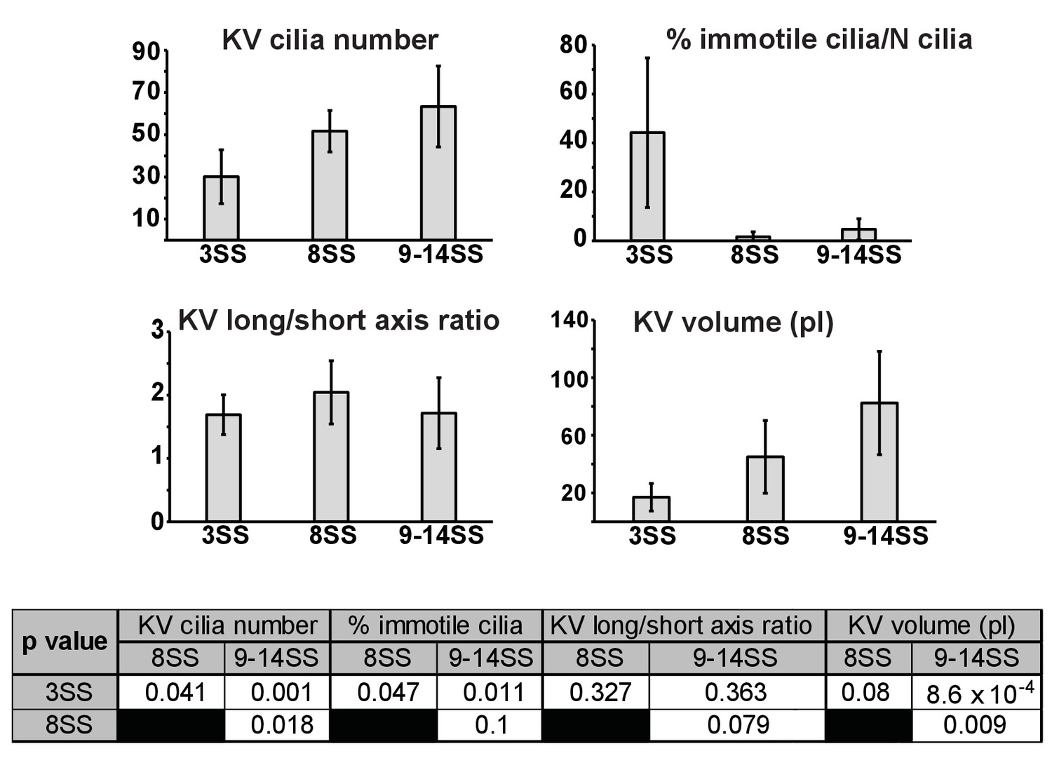
Quantification of KV and cilia features comparing the 3-, 8- and 9–14-somite stage (SS).
Table p-values (see more features in Table 1).
Figure 4—figure supplement 2
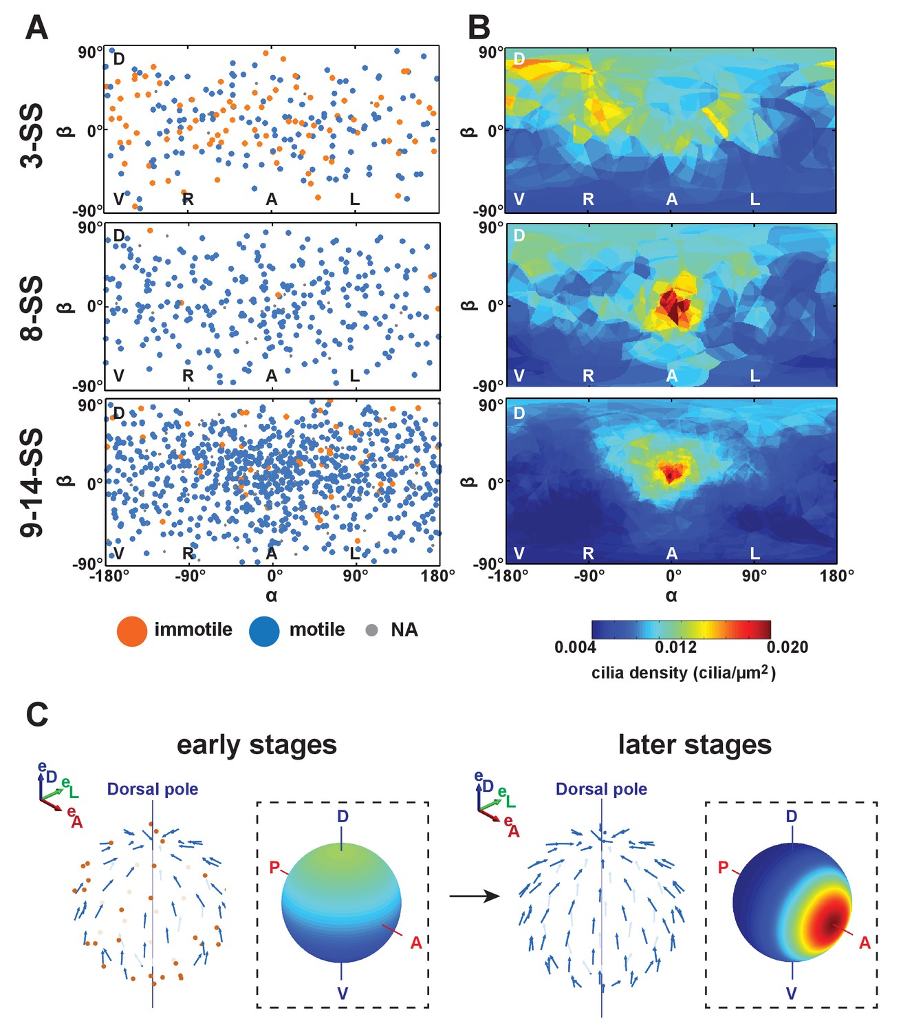
Changes in cilia spatial distribution and orientation over time.
(A) Spatial distribution in 2D maps of immotile (blue) and motile (orange) cilia. Between 3- and 9–14-somite stage (SS), the proportion of immotile cilia decreases from 44% to 5% (see also Table 1). (B) Cilia density maps show an enrichment at the anterior pole (°) that accumulates over time (from 3- to 9–14-SS). (C) Scheme summarizing the main differences in cilia 3D orientation and density map (dashed boxes) between early (3-SS, left) and late (9- to 14-SS, right) stages of development: while early vesicles contain many immotile cilia (red), motile cilia (blue) always exhibit a meridional tilt at both early and late stages. The cilia density map is first dominated by a dorsal gradient before exhibiting a strong anterior gradient at late stages (color map from blue to red representing low to high cilia density). See Figure 1 for the definition of the body plan reference frame and coordinates systems.
Figure 5
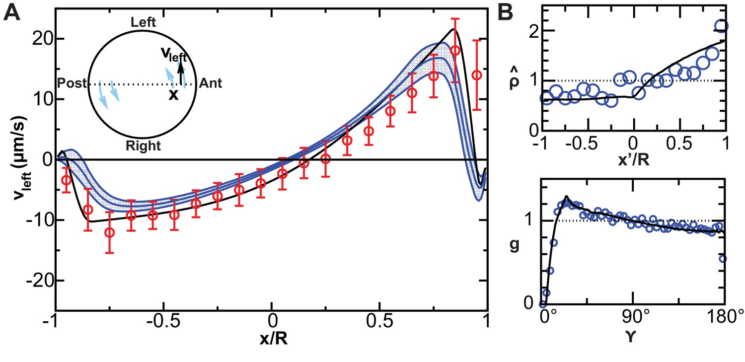
Validation of calculated flow profiles.
(A) Velocity profile along the anteroposterior (AP) axis (anterior: ; posterior: ), positive values indicate leftward flow. Red: experimental values obtained with particle tracking (Supatto et al., 2008). Blue: calculated flows using observed cilia distributions from vesicles from 8-somite stage (SS) to 14-SS (mean ± std. error; ). Black: simulations using randomly generated cilia distributions. (B) Statistical features used to generate cilia distributions (blue circles: experimental distributions, black line: model). Top panel: normalized surface density as a function of the position along the tilted AP axis ( at the point with maximum density, ); bottom panel: pair correlation function as a function of the angular distance between two cilia. number of vesicles.
Figure 6 with 1 supplement
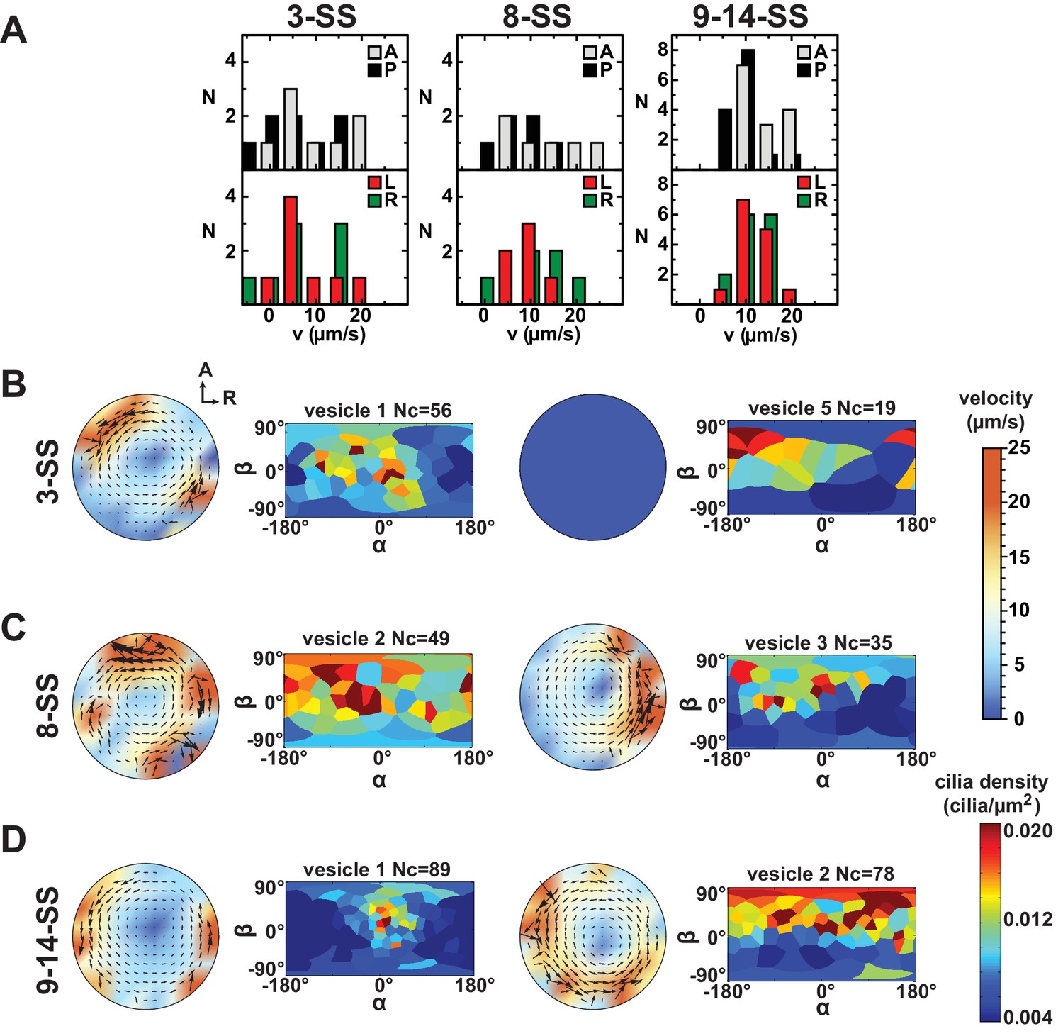
Variability in cilia distributions and flow profiles between individual Kupffer’s vesicle (KV) at 3-, 8- and 9–14- somite stage (SS):
(A) Distributions of flow velocities in individual KV at 3-, 8- and 9–14-SS. The upper panel shows the mean velocities in the regions around the anterior (A) and posterior (P) poles and the lower panel around the left (L) and right (R) poles. (B–D) Flow profiles and 2D cilia density maps for two representative KV at 3-SS (B), 8-SS (C) and 9–14-SS (D) (see Figure 6—figure supplement 1 for all individual KV).
Figure 6—figure supplement 1
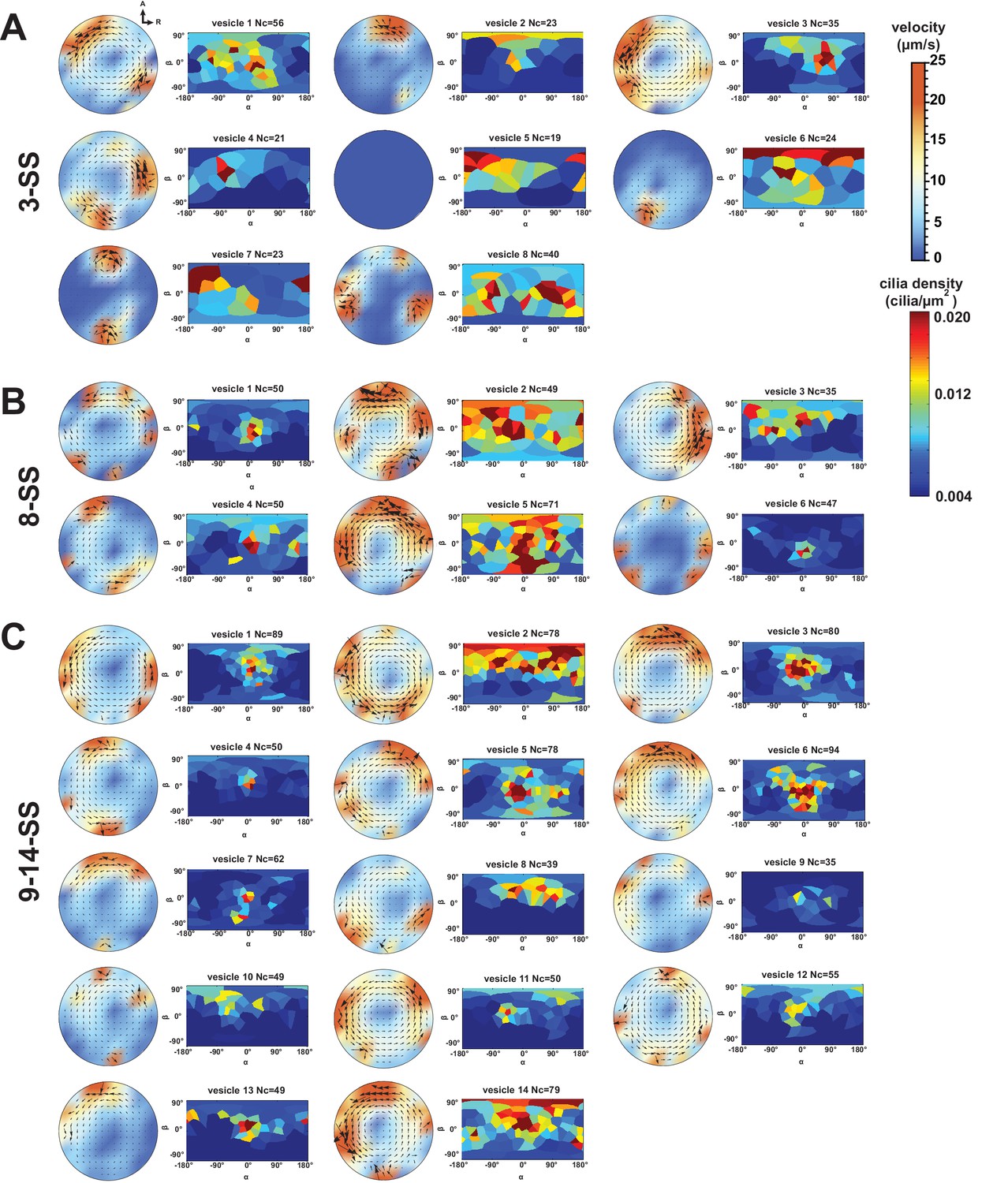
Flow profiles and 2D cilia density maps for all Kupffer’s vesicles (KV) analyzed at 3- somite stage (SS) (A), 8-SS (B) and 9–14-SS (C), showing a great variability between embryos.
https://doi.org/10.7554/eLife.25078.013
Figure 7 with 1 supplement
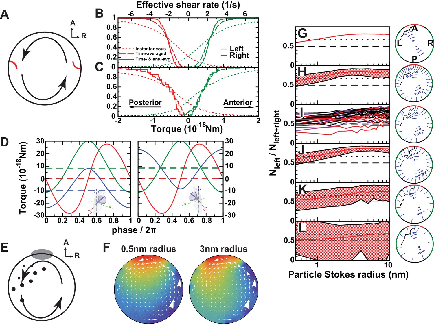
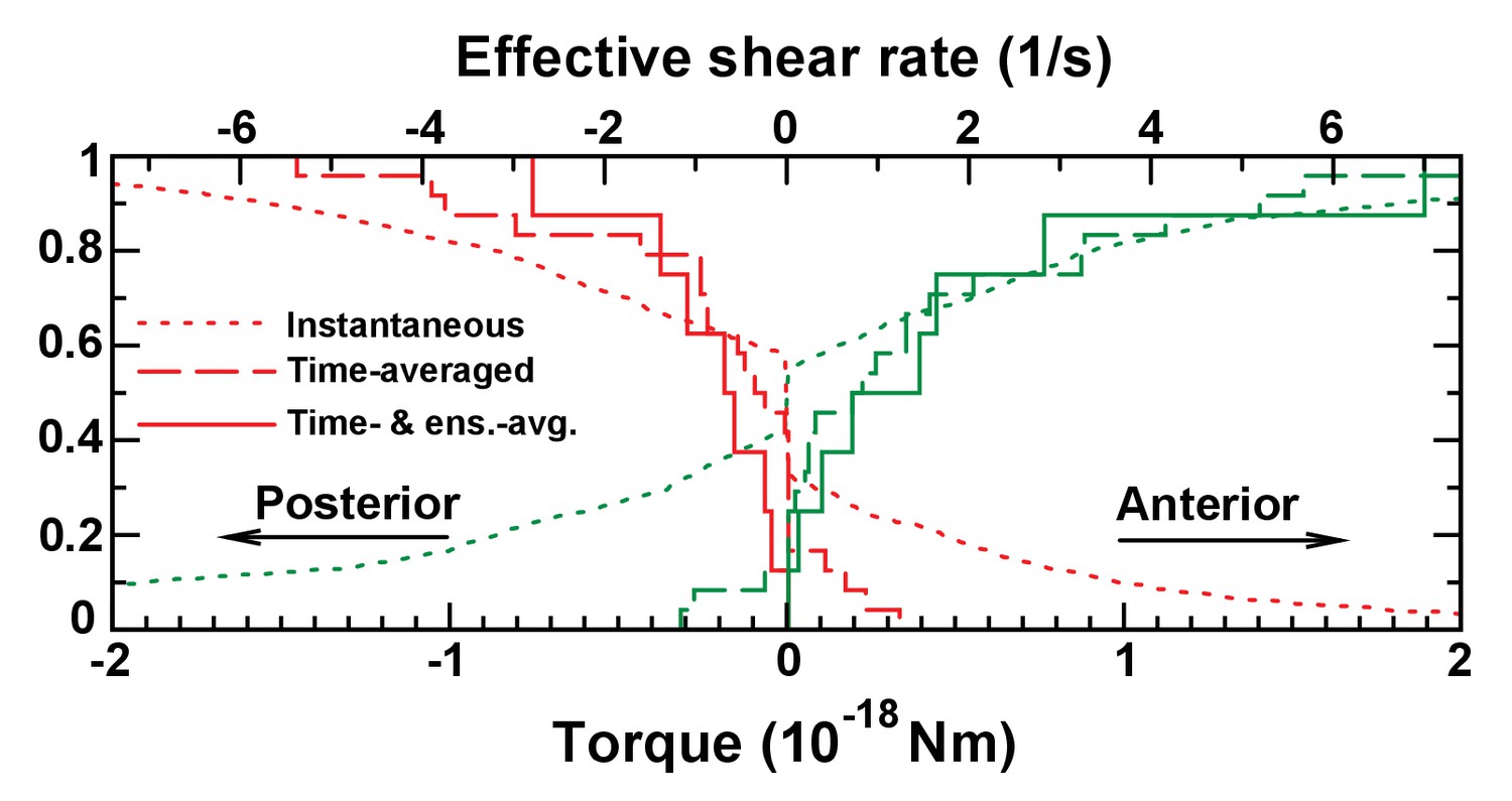
Physical limits of possible side detection mechanisms.
(A) Mechanosensory mechanism 1: directional flow sensing. Sensory cilia (red) on the left (L) and on the right (R) side are deflected by the rotational flow (arrows). They must be able to distinguish between anterior- and posterior-directed flows. (B–C) Cumulative fraction of cilia with the anterior acting force below (right, green) or above (left, red) the value on the abscissa. The dotted lines show instantaneous values (blurred by oscillatory flows of adjacent cilia), dashed lines show the temporal average, and the continuous line the temporal and ensemble average of 3 immotile cilia on each side. The diagrams show the results on randomly generated (B) and experimentally characterized (C) vesicles. The results show that reliable detection (<5% error) would need a sensitivity threshold of 1 × 10⁻¹⁹ Nm. The upper scale shows the effective flow shear rate above a planar surface that induces the equivalent torque on an isolated passive cilium of the same length. (D) Mechanosensory mechanism 2: detection of a cilium's own movement. According to this mechanism, a cell can sense the torque components caused by the motion of its active cilium through the viscous fluid. The lines show the meridional component towards posterior (blue), parallel component towards dorsal (red), and normal component (green). The meridional component shows a temporal average of 10−17 Nm that could potentially allow discrimination between left (left panel) and right (right panel) side. (E) Chemosensory mechanism, based on flow mediated transport of a signaling molecule. Particles are secreted from a region 30° around the anterior (A) pole and then travel diffusively through the rotating fluid. They get absorbed upon encounter with any cilium outside the anterior region. Eventually, particles absorbed in a 45° region around left-right poles are counted. (F) Average particle concentration (arbitrary units) in the equatorial plane for particles where diffusion dominates fluid circulation (Stokes radius = 0.5 nm, top) and those with drift dominating (3 nm, bottom). In the latter case, an asymmetry in the distribution is clearly visible (Video 3). (G–L) Fraction of particles counted on the left among the total count of left and right for different scenarios. The dotted line shows a proposed detection threshold with a left to right ratio of 2:1. The red line shows the average vesicle and the shadowed region the interval between the 5th and the 95th percentile. (G) Continuous model with uniform circulation (Ω = 0.5 s−1). (H) Randomly generated cilia distributions with natural parameters. (I) Simulation on individual vesicles at 3-SS (red), 8-SS (indigo) and 9–14-SS (black). (J) Same as H, but homogeneous cilia distribution. (K) Same as H, but reduced number of cilia (). (L) Further reduced number of cilia (). The following figure supplement is available for Figure 7.
Figure 7—figure supplement 1
Cumulative torque distributions on immotile cilia as in Figure 7C, but using cilia maps at 3-somite stage.
https://doi.org/10.7554/eLife.25078.016Videos
Video 1
Visualization of the 3D-CiliaMap processing workflow from 3D live imaging to Kupffer’s vesicle (KV) surface segmentation and cilia vectorization.
Firstly, one embryo from the Tg (actb2:Mmu.Arl13b-GFP) (Borovina et al., 2010) line soaked for 60 min in Bodipy TR (Molecular Probe) is imaged using 2-photon excitation fluorescence (2PEF) microscopy at 930 nm wavelength. A full z-stack of the KV can be seen. Subsequently, using Imaris (Bitplane Inc.), z-stacks are rendered into 3D volume and the KV cell surface is manually segmented so that only cilia at the cell surface surrounding the KV are visible. At the end, we show the cilia vectorized in the whole volume imaged after 2PEF acquisition.
Video 2
3D visualization of the calculated average flows at 3-somite-stage (SS) (left), 8-SS (center) and 9–14-SS (right).
See Figure 4B for the velocity color scale. The axes show the direction of anterior (red), left (green) and dorsal (blue). At all stages the average flow is directional around the dorsoventral (DV) axis, but the flow velocity increases between 3- and 9–14-SS. The flow profiles in the anteroposterior (AP)-left-right (LR) plane are shown in Figure 4B.
Video 3
Simulated transport of signaling molecules in the Kupffer’s vesicle (KV).
Panoramic view of the KV as seen from the center. The cilia distribution is obtained from vesicle 1 at 9–14-somite stage (Figure 6—figure supplement 1C). Cilia shown in blue are motile and those in red immotile or undetermined. Signaling particles (, not to scale), secreted from anterior (yellow), are subject to Brownian motion biased by the leftward flow until they are absorbed by a cilium (shown yellow after particle capture). 10 s of video represent 1s real time. Link for 360° video: https://youtu.be/1caSzBIe5rA
Tables
Table 1
Statistical properties of all KV analyzed. Table summarizing some of the cilia features collected from the 3D-CiliaMap for individual KV at 3-, 8- and 9–14- somite stage (SS).
| stage | KV number | N cilia | % immotile cilia | Ellipsoid axis | Axis ratio a / b | Volume (pl) | Average motile cilium | Ellipsoid fit RMS residue (µm) | Ω (s-1) | |||
|---|---|---|---|---|---|---|---|---|---|---|---|---|
| a (µm) | b (µm) | r | θ (°) | φ (°) | ||||||||
| 3-SS | 1 | 56 | 11% | 27 | 12 | 2.3 | 35 | 0.8 | 37 | 6 | 2.07 | 0.423 |
| 2 | 23 | 39% | 21 | 12 | 1.8 | 21 | 0.8 | 44 | 2 | 1.56 | 0.207 | |
| 3 | 35 | 3% | 23 | 12 | 1.9 | 27 | 0.8 | 42 | -11 | 2.38 | 0.457 | |
| 4 | 21 | 33% | 18 | 11 | 1.6 | 15 | 0.8 | 22 | 12 | 2.14 | 0.350 | |
| 5 | 19 | 100% | 15 | 9 | 1.7 | 8 | NA | NA | NA | 1.5 | 0.000 | |
| 6 | 24 | 54% | 15 | 10 | 1.5 | 9 | 0.7 | 28 | 3 | 1.78 | 0.230 | |
| 7 | 23 | 61% | 14 | 12 | 1.2 | 10 | 0.8 | 18 | -46 | 1.92 | 0.110 | |
| 8 | 40 | 53% | 18 | 11 | 1.6 | 16 | 0.7 | 8 | 22 | 2.05 | 0.034 | |
| mean ± SD | 30 ± 13 | 44% ± 31% | 19 ± 5 | 11 ± 1 | 1.7 ± 0.3 | 17 ± 10 | 0.8 ± 0.1 | 28 ± 13 | -2 ± 22 | 1.9 ± 0.3 | 0.226 ± 0.173 | |
| 8-SS | 1 | 50 | 4% | 29 | 18 | 1.6 | 64 | 0.8 | 37 | -14 | 1.2 | 0.270 |
| 2 | 49 | 2% | 22 | 8 | 2.8 | 15 | 0.8 | 35 | 6 | 1.1 | 0.595 | |
| 3 | 43 | 0% | 25 | 11 | 2.3 | 30 | 0.7 | 46 | 12 | 2.3 | 0.561 | |
| 4 | 50 | 4% | 27 | 12 | 2.3 | 39 | 0.7 | 41 | 16 | 2.5 | 0.329 | |
| 5 | 71 | 0% | 26 | 13 | 2.0 | 36 | 0.8 | 35 | 16 | 1.8 | 0.469 | |
| 6 | 47 | 0% | 30 | 22 | 1.4 | 85 | 0.7 | 21 | 39 | 1.7 | 0.110 | |
| mean ± SD | 52 ± 10 | 2% ± 2% | 26 ± 3 | 14 ± 5 | 2.0 ± 0.5 | 45 ± 25 | 0.7 ± 0.1 | 36 ± 8 | 13 ± 17 | 1.7 ± 0.5 | 0.389 ± 0.186 | |
| 9-14-SS | 1 | 89 | 16% | 37 | 31 | 1.2 | 174 | 0.7 | 49 | 12 | 2.1 | 0.271 |
| 2 | 78 | 6% | 27 | 15 | 1.8 | 47 | 0.7 | 46 | 18 | 2.0 | 0.600 | |
| 3 | 80 | 3% | 33 | 20 | 1.7 | 93 | 0.8 | 54 | 13 | 2.2 | 0.412 | |
| 4 | 50 | 0% | 33 | 20 | 1.7 | 91 | 0.7 | 47 | 14 | 2.6 | 0.290 | |
| 5 | 78 | 6% | 31 | 17 | 1.8 | 70 | 0.7 | 36 | 20 | 2.0 | 0.393 | |
| 6 | 94 | 4% | 36 | 21 | 1.7 | 111 | 0.8 | 52 | 10 | 1.7 | 0.424 | |
| 7 | 62 | 11% | 34 | 26 | 1.3 | 124 | 0.8 | 46 | 11 | 1.8 | 0.216 | |
| 8 | 39 | 3% | 24 | 20 | 1.2 | 48 | 0.7 | 54 | 36 | 4.4 | 0.378 | |
| 9 | 35 | 0% | 31 | 13 | 2.4 | 52 | 0.8 | 50 | 10 | 2.6 | 0.245 | |
| 10 | 49 | 4% | 32 | 17 | 1.9 | 74 | 0.8 | 53 | 2 | 2.3 | 0.275 | |
| 11 | 50 | 2% | 30 | 22 | 1.4 | 82 | 0.9 | 64 | 3 | 2.9 | 0.433 | |
| 12 | 55 | 2% | 30 | 23 | 1.3 | 85 | 0.8 | 61 | 11 | 2.6 | 0.388 | |
| 13 | 49 | 4% | 33 | 10 | 3.3 | 47 | 0.7 | 40 | 32 | 2.1 | 0.224 | |
| 14 | 79 | 5% | 27 | 19 | 1.4 | 56 | 0.7 | 51 | 22 | 1.8 | 0.521 | |
| mean ± SD | 63 ± 19 | 5% ± 4% | 31 ± 4 | 19 ± 5 | 1.7 ± 0.6 | 82 ± 36 | 0.8 ± 0.05 | 50 ± 7 | 15 ± 10 | 2.3 ± 0.7 | 0.362 ± 0.114 | |
Table 2
List of symbols: Quantities and their values with sources where applicable.
| Symbol | Description | From 3D-CiliaMap | Value: standardized vesicle |
|---|---|---|---|
| Cilium's coordinate system | + | ||
| KV coordinate system | + | ||
| Coordinate | + | ||
| Coordinate | + | ||
| Cilium tilt | + | ||
| Cilium orientation on the cell surface | + | 0 | |
| Cilium, semi-cone angle | |||
| Cilium, angular frequency | |||
| Cilium, length | |||
| KV radius | + | ||
| KV ellipsoid, equatorial radius | + | ||
| KV ellipsoid, height | + | ||
| Number of cilia | + | 70 | |
| Surface density of cilia | + | ||
| Normalized surface density of cilia | + | See Figure 5 | |
| Cilia distribution, pair correlation | + | See Figure 5 | |
| Fluid viscosity | |||
| Diffusive particle Stokes radius | |||
| Particle diffusion constant | |||
| Fluid velocity inside KV | calculated | ||
| Effective flow angular velocity | calculated | ||
| Number of particles captured on the left/right | simulated | ||
Additional files
-
Source code 1
Matlab script describing the structure of KVdata.mat information (see script comments) and displaying a sample figure of cilia distribution in a vesicle to show how to use this MAT-file.
- https://doi.org/10.7554/eLife.25078.019
-
Source code 2
“KVdata.mat” is a MAT-file containing all vesicle features computed in this study (see Source code 1 for information about its content and use).
- https://doi.org/10.7554/eLife.25078.020
Download links
A two-part list of links to download the article, or parts of the article, in various formats.
Downloads (link to download the article as PDF)
Open citations (links to open the citations from this article in various online reference manager services)
Cite this article (links to download the citations from this article in formats compatible with various reference manager tools)
Physical limits of flow sensing in the left-right organizer
eLife 6:e25078.
https://doi.org/10.7554/eLife.25078


