Figures and data in Ionic mechanisms underlying history-dependence of conduction delay in an unmyelinated axon

Figures
Tables

12 figures and 2 tables

Figures

Figure 1

Download asset Open asset

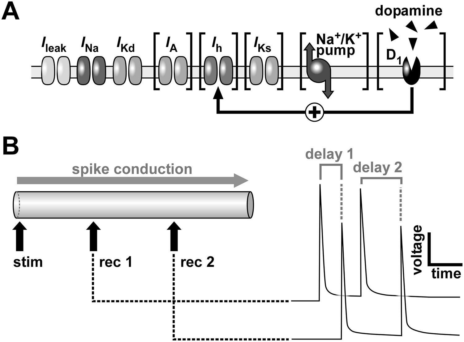
Schematic of the model axon and conduction delay.

(A) Schematic of ion channels, the Na⁺/K⁺ pump and dopamine receptors in the model axon. Brackets indicate components that were omitted in some simulations. (B) The model axon was stimulated at one end and the conduction delay was measured between two positions at 0.3 and 0.7 times the length of the axon. Right panel shows conduction delays between the recording sites for two consecutive action potentials.

https://doi.org/10.7554/eLife.25382.002

Figure 2

Download asset Open asset

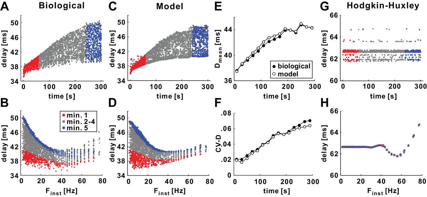
History-dependence of conduction delay in the model axon (with *g_h* = 0).

(A) Delay shown as a function of stimulus time for a 10 Hz (mean rate), 5 min *Poisson* stimulation of the axon of the biological PD neuron. Red and blue, respectively, mark delay values for the first and fifth minute of stimulation. (B) The data in panel A, plotted as a function of the instantaneous stimulus frequency (F_inst). Colors as in panel A. (**C–D**) The same *Poisson* stimulation as in panel A, applied to the model axon produces results that are quantitatively similar to the experimental data. (**E–F**) The mean (D_mean) and the coefficient variation (CV-D) of the data in panels A and C, measured in 20 s bins. (**G–H**) The same *Poisson* stimulation of panels *C-D*, applied to the standard Hodgkin-Huxley model axon.

https://doi.org/10.7554/eLife.25382.003

Figure 3

Download asset Open asset

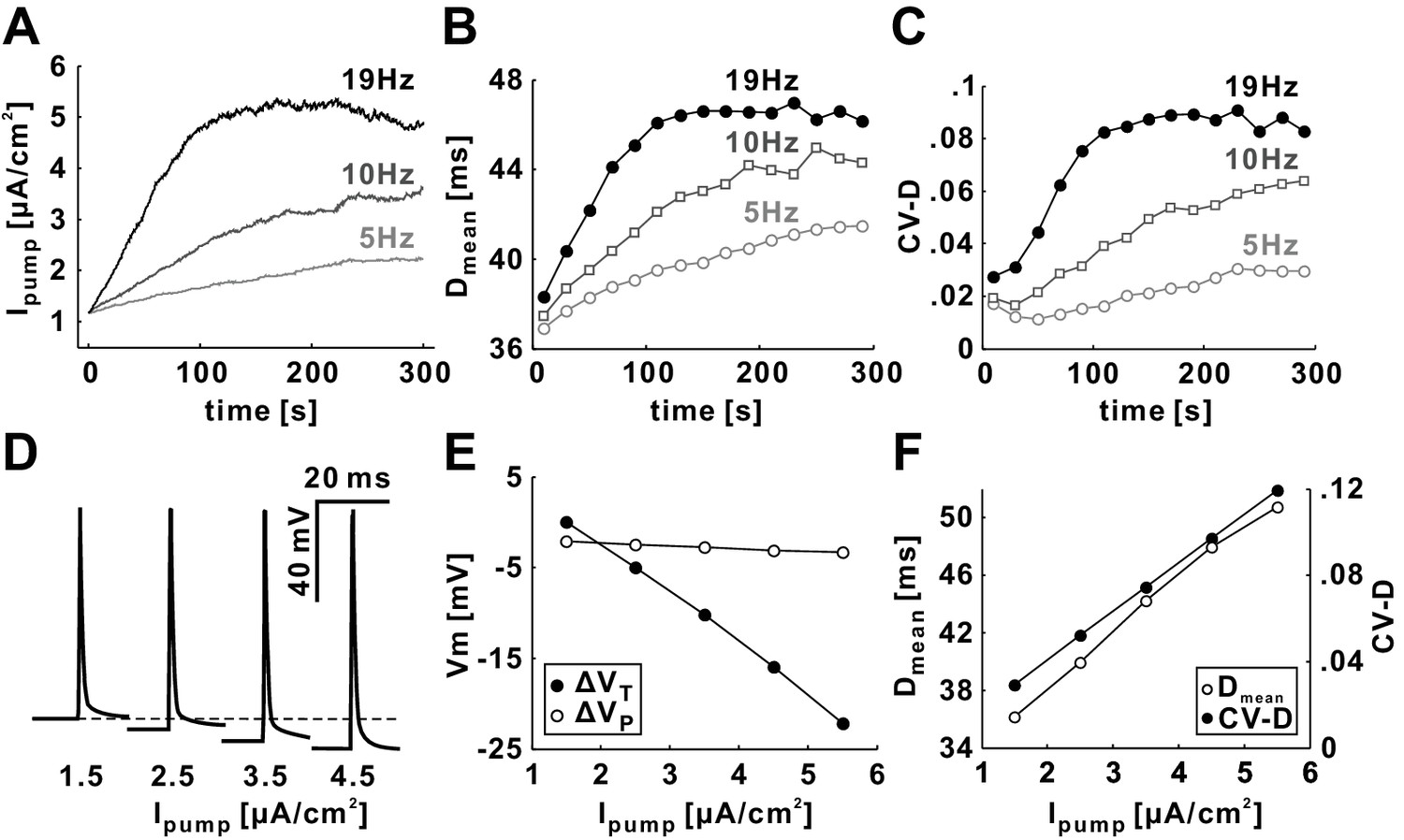
D_mean and CV-D strongly depend on the activity level of *I_pump* at all *Poisson* stimulation frequencies.

(A) The value of *I_pump* for *Poisson* stimulations with different mean rates (5, 10 and 19 Hz). (**B–C**) D_mean and CV-D increase with time as well as with the mean rate of *Poisson* stimulation. (D) The baseline membrane potential is hyperpolarized as the level of *I_pump* is increased. (E) The trough voltage (V_T) linearly decreases with *I_pump*, but the peak voltage (V_P) does not change much when *I_pump* is increased. (F) D_mean and CV-D linearly increase with the level of *I_pump* (set to a constant value in each simulation run).

https://doi.org/10.7554/eLife.25382.004

Figure 4

Download asset Open asset

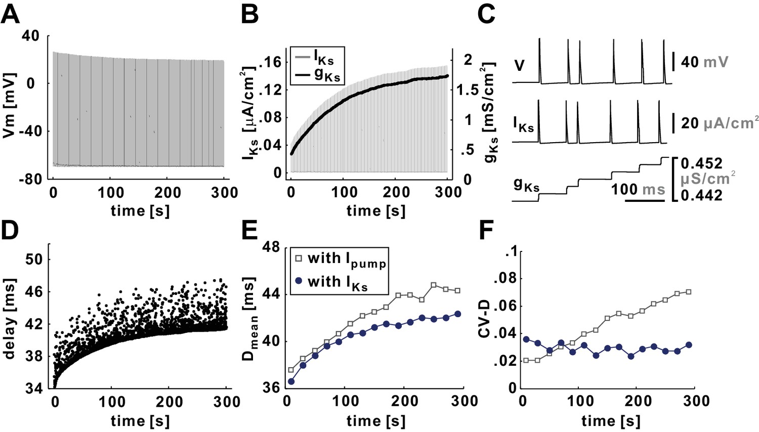
A slow potassium current (*I_Ks*) fails to capture the slow timescale effects on conduction delay.

(A) Voltage trace of the model axon, with *I_Ks* substituted for *I_pump*, for a 5 min, 10 Hz *Poisson* stimulation. (B) Both *g_Ks* and the peak values of *I_Ks* increase with time during the stimulation process. (C) A small time-window shows that, although *g_Ks* accumulates with time, *I_Ks* vanishes after each action potential because of the drop in the driving force. (D) Conduction delay of the model axon in response to a 5 min, 10 Hz *Poisson* stimulation. (E) D_mean increases with time but does not quite match the results of the model axon with *I_pump*. (F) CV-D does not increase with time as it does in the model axon with *I_pump*.

https://doi.org/10.7554/eLife.25382.005

Figure 5

Download asset Open asset

Changing the level of *I_h* in the model mimics the experimental effects of CsCl and DA.

(**A1–B1**) At the slow timescale, DA results in an increase of *g_h*, which in turn causes D_mean and CV-D stay to remain relatively constant in response to a 5 min 10 Hz *Poisson* stimulation. In contrast, blocking *I_h* with CsCl results in an increase in D_mean and CV-D (Ballo et al., 2012). (**A2–B2**) This effect is mimicked by changing *g_h* levels and the activation curve of *I_h* in the model. (C1) Changes in *g_h* levels by DA or CsCl result in changes in the minimum delay (D_min) and curvature (κ_min) values in the delay vs. F_inst plots (for the 5^th minute of the *Poisson* stimulation). (C2) These effects are mimicked by the models with different activity level of *I_h* (see Materials and methods and Tables 1 and 2 for details).

https://doi.org/10.7554/eLife.25382.006

Figure 6

Download asset Open asset

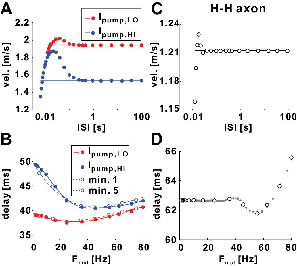
The fast timescale effect can be predicted by paired-pulse stimulations.

(A) Conduction velocity of conditioning (horizontal line) and test (filled circles) pulses plotted as a function of interspike interval (ISI). The graph shows the refractory and supernormal phases, where the velocity of the test pulse is, respectively, less or more than that of the conditioning pulse. Simulations were done with two constant pump currents: *I_pump,*_LO and *I_pump,*_HI, respectively equal to the mean value of *I_pump* during minute 1 and minute 5 of the 10 Hz *Poisson* stimulation (Figure 2). Horizontal lines show the velocity of the conditioning spikes. (B) Data of panel A plotted as conduction delay vs. F_inst (=1/ISI), together with the *Poisson* stimulation results of minutes 1 and 5 (from Figure 2D). Solid curves are polynomial fits for the *I_pump,LO* and *I_pump,HI* datasets. (C) Paired-pulse stimulations of the Hodgkin-Huxley model axon show similar refractory and supernormal phases. (D) The data from the panel C compared with the *Poisson* stimulation data (from Figure 2H) of the Hodgkin-Huxley model axon show a perfect match.

https://doi.org/10.7554/eLife.25382.009

Figure 7

Download asset Open asset

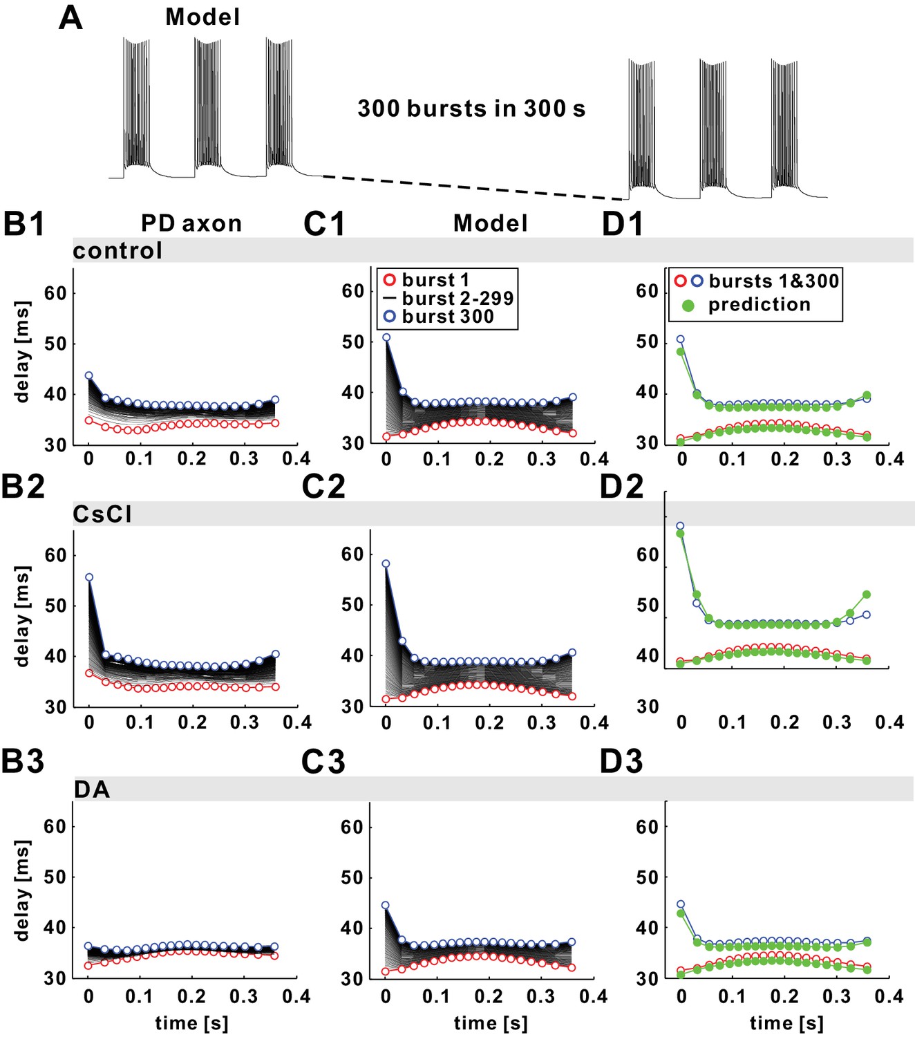
The fast timescale effect observed in the burst stimulations can be predicted by the paired-pulse stimulation results.

(A) The model responses to 300 parabolic burst stimuli (350 ms duration; 1 s period) over 300 s show a drop in baseline membrane potential. (**B1–B3**) Experimental results of conduction delay of spikes in each burst shown, superimposed as a function of time from the burst onset. Data of the first (red) and the 300th (blue) burst are colored. (**C1–C3**) Model replication of the experimental results, with different *I_h* levels (see Tables 1 and 2 for model parameters). (**D1–D3**) Simulation results of the first and the 300th burst in panel *C1-C3* are predicted by estimating history-dependence using paired-pulse simulations (see Figure 6). Paired-pulse simulations were done with a constant low or high *I_pump* level, equal, respectively, to the *I_pump* mean value during the first and the 300th burst, fit with polynomial functions and used to obtain the plotted predictions (green).

https://doi.org/10.7554/eLife.25382.010

Figure 8

Download asset Open asset

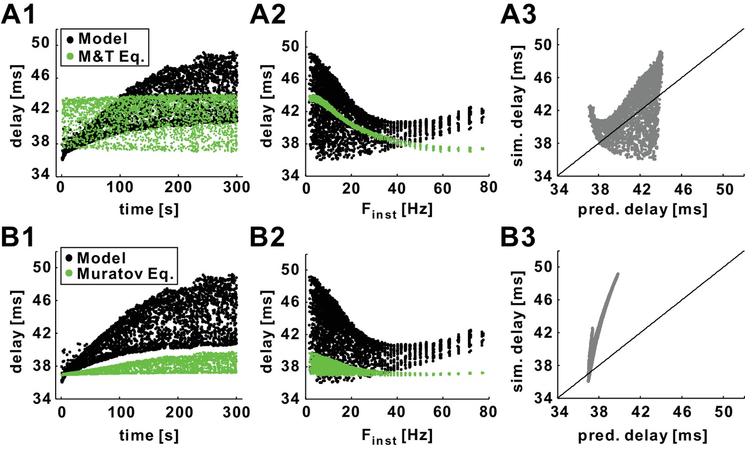
Predictions of history-dependence of conduction delay by previously published equations of action potential velocity.

(A1) Conduction delays of the biophysical model in response to 10 Hz *Poisson* stimulation and delays predicted by the Matsumoto and Tasaki equation (Tasaki and Matsumoto, 2002). (A2) Data in panel A1 plotted versus F_inst. (A3) Simulation delay versus delay predicted by Matsumoto and Tasaki equation. (**B1–B3**) Comparison between simulation delays in the biophysical model (as in *A1-C1*) and the delays predicted by the Muratov equation (Muratov, 2000). Diagonal lines are y=x.

https://doi.org/10.7554/eLife.25382.011

Figure 9

Download asset Open asset

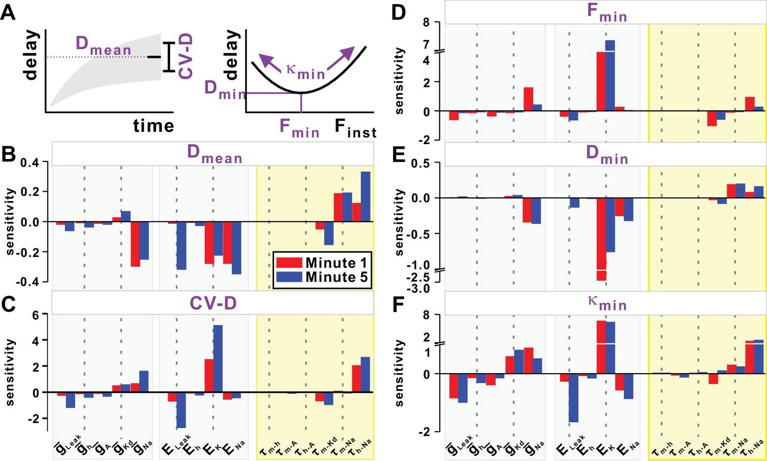
Sensitivity of the slow (STS) and fast timescale (FTS) effects to the model parameters.

(A) Top left inset schematically shows the mean (D_mean) and variability of conduction delay (CV-D = coefficient of variation), measured in the last 20 s of simulation. Top right inset schematically shows the minimum delay point (F_min, D_min) and the curvature κ_min of the quadratic fit at this point. (**B–C**) STS effect. Sensitivity of D_mean and CV-D to model parameters in the first and five minute of a 10 Hz *Poisson* stimulation. (**D–F**) FTS effect. Sensitivity of F_min, D_min and κ_min to model parameters in the first and fifth minute of a 10 Hz *Poisson* stimulation.

https://doi.org/10.7554/eLife.25382.012

Figure 10

Download asset Open asset

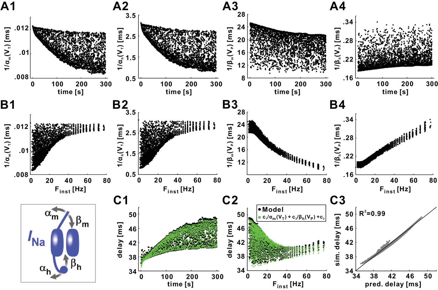
Conduction delay is determined by the *I_Na* activation and inactivation variables, evaluated at the action potential trough (*V_T*) or peak (*V_P*) voltage.

(**A1–A2**) Reciprocal of the *I_Na* activation rate, evaluated at *V_T*. (**A3–A4**) Reciprocal of the *I_Na* inactivation rate, evaluated at *V_P*. (**B1–B4**) Data in panel A plotted as a function of F_inst. (C1) Conduction delay of the model compared with the predicted delay of c₁/*α_m*(*V_T*)+c₂/*β_h*(*V_P*)+c₃ (c₁ = −3361.48, c₂ = 32.80, c₃ = 70.14). (C2) Data in panel C1 plotted as a function of F_inst. (C3) Simulation delays compared with predicted delays from the empirical equation (R²=0.99). The line is y=x. The inset is the schematic of the fast sodium channel.

https://doi.org/10.7554/eLife.25382.013

Figure 11

Download asset Open asset

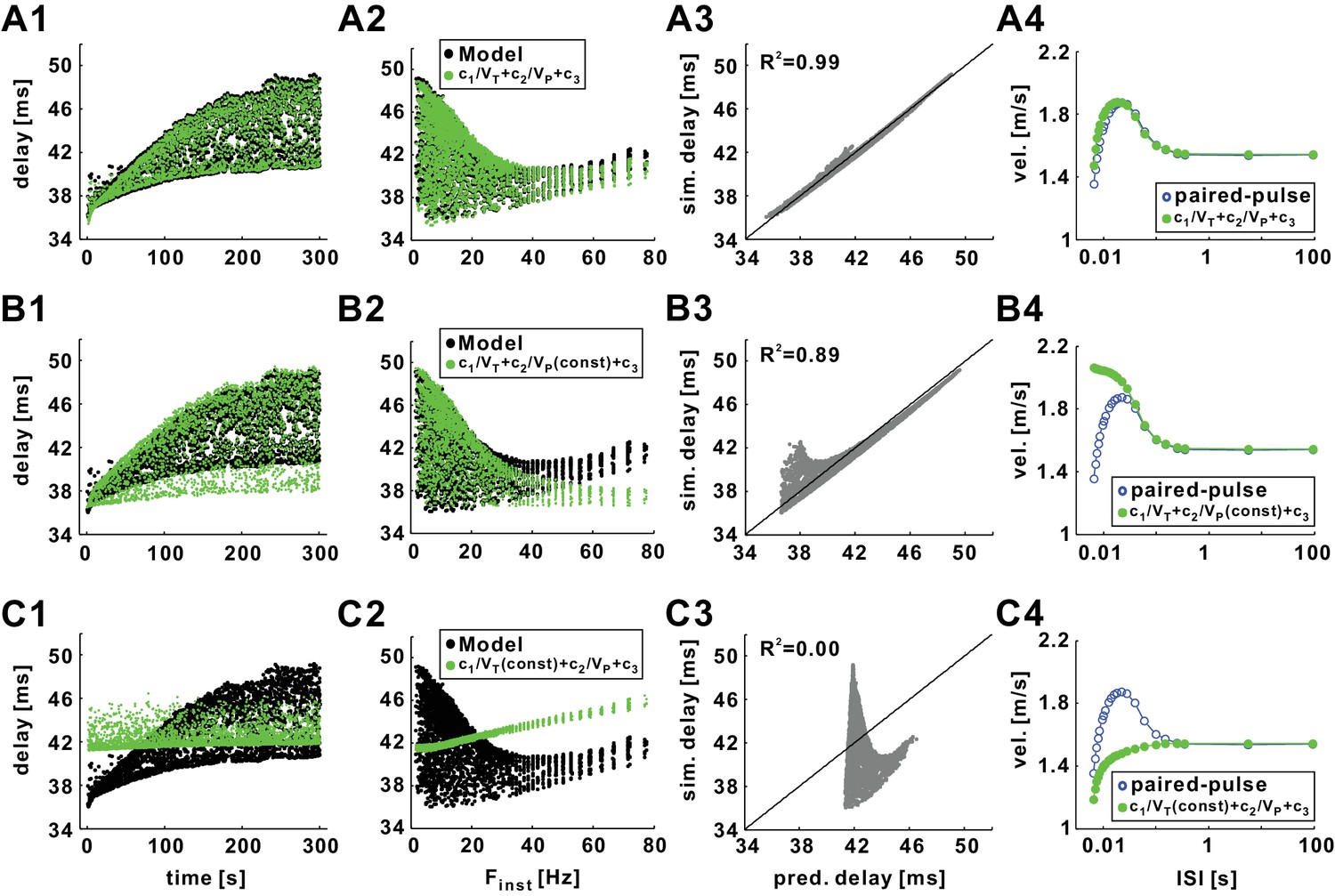
Conduction delay can be almost perfectly predicted by the trough and peak voltages of the action potentials.

(A1) Superimposed graph of conduction delays of the biophysical model (black) in response to 10 Hz *Poisson* stimulation and the predicted delays from the nonlinear regression equation: d = c₁/*V_T* +c₂/*V_P* +c₃ (c₁ = 4072.88, c₂ = 302.36, c₃ = 82.94; the same values of c₁-c₃ are used in all panels). (A2) Data in panel A1 plotted as a function of F_inst. (A3) Simulation delays (training data) compared with predicted delays (R² = 0.99). (A4) Conduction delays of the biological model (blue) in response to paired-pulse stimulation (same as in Figure 6A) and the predicted delays from the regression equation in panel A1. (**B1–B3**) Simulation results (same as in *A1-A3*) compared with predicted delays from the single variable regression: d = c₁/*V_T* +c₂/*V_P* (mean) +c₃, where *V_P* (mean) is the mean value of *V_p*. (B4) Simulation results (same as in A4) compared with predicted delays from the single variable regression: d = c₁/*V_T* +c₂/*V_P* (cond) +c₃, where *V_P* (cond) is the value of *V_p* of the conditioning pulse. (**C1–C3**) Simulation results (same as in *A1-A3*) compared with predicted delays from the single variable regression: d = c₁/*V_T*(mean)+c₂/*V_P* +c₃, where *V_T* (mean) is the mean value of *V_T*. The lines in A3, B3, and C3 are y=x. (C4) Simulation results (same as in A4) compared with predicted delays from the single variable regression: d = c₁/*V_T*(cond)+c₂/*V_P* +c₃, where *V_T* (cond) is the value of *V_T* of the conditioning pulse.

https://doi.org/10.7554/eLife.25382.014

Figure 12

Download asset Open asset

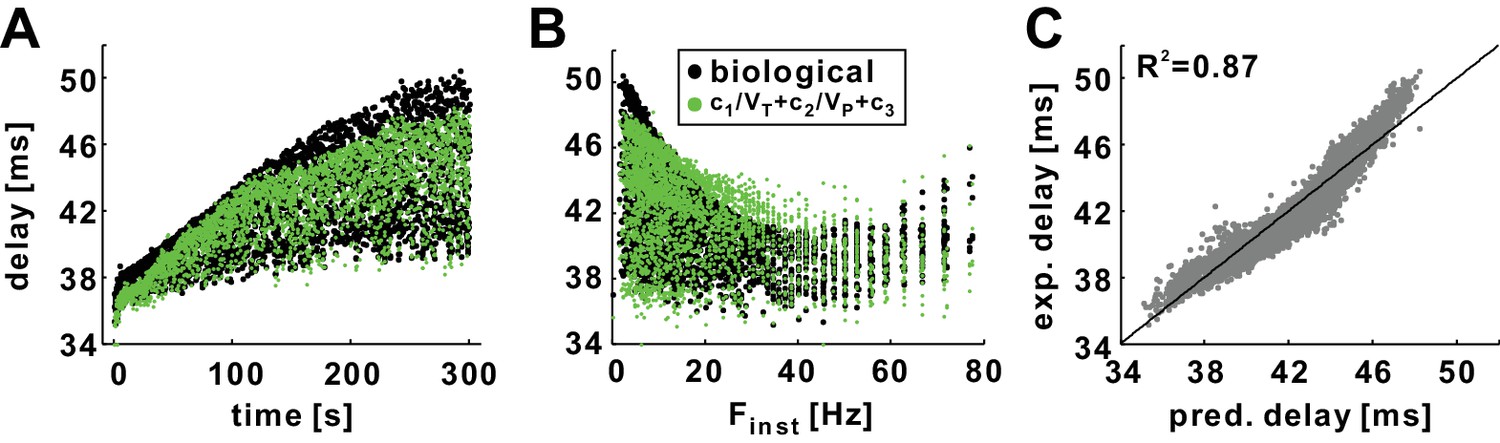
The history dependence of conduction delay in the biological PD axon can be predicted by the empirical equation without need for computational modeling.

(A) Conduction delays in the biological PD axon in response to a 5 min, 10 Hz, *Poisson* stimulation (black; same as in Figure 2A) compared with delays predicted by empirical equation (c₁=4817.75, c₂ = 500.5, c₃ = 105) using *V_T* and *V_P* values from intracellular recordings (not shown). (B) Data in panel A plotted as a function of F_inst. (C) Experimental delays plotted versus the predicted delays (R² = 0.87). The line is y=x.

https://doi.org/10.7554/eLife.25382.015

Tables

Table 1

Model parameters.

https://doi.org/10.7554/eLife.25382.007

Ionic Curr	${\bar{g}}_{x}$ [mS/cm²]	$E_{x}$ [mV]
I_Na	14	Dynamic
I_Kd	3	−70
I_Leak	0.125	−65
I_A	5	−70
I_h (ctrl)	0.05	−32
I_h (DA)	0.1	−25
I_Ks	3	−70
*Other*	*Value*
I_max,pump	2 mA/cm²
[Na⁺]_1/2	78 mM
[Na⁺]_S	2 mM
α	7.4
Vol	7850 µm³
F	96485 C/mol

Table 2

Parameters of ionic current steady-state activation and inactivation and their time constants.

https://doi.org/10.7554/eLife.25382.008

Ionic Curr	m, h	$x_{\infty}$	$τ_{x}$ [ms]
I_Na	m³	$\frac{1}{1 + \exp (- (V + 48) / 8.5)}$	$\frac{0.132}{\cosh ((V + 27) / 7.5)} + \frac{0.003}{1 + \exp (- (V + 27) / 5)}$
I_Na	h	$\frac{1}{1 + \exp ((V + 47) / 6)}$	$\frac{10}{\cosh ((V + 42) / 15)}$
I_Kd	m⁴	$\frac{1}{1 + \exp (- (V + 47) / 10)}$	$\frac{50}{\cosh ((V + 73) / 15)}$
I_A	m³	$\frac{1}{1 + \exp (- (V + 63) / 15)}$	$18 + \frac{58}{1 + \exp ((V + 61) / 20)}$
I_A	h	$\frac{1}{1 + \exp ((V + 80) / 8)}$	50
I_h (ctrl)	m	$\frac{1}{1 + \exp ((V + 80) / 5.5)}$	3700
I_h (DA)	m	$\frac{1}{1 + \exp ((V + 75) / 12.5)}$	3800
I_Ks	m	$\frac{1}{1 + \exp (- (V + 47) / 10)}$	$\frac{250000}{\cosh ((V + 73) / 15)}$

Download links

A two-part list of links to download the article, or parts of the article, in various formats.

Downloads (link to download the article as PDF)

Article PDF

Open citations (links to open the citations from this article in various online reference manager services)

Mendeley

Cite this article (links to download the citations from this article in formats compatible with various reference manager tools)

Yang Zhang
Dirk Bucher
Farzan Nadim

(2017)

Ionic mechanisms underlying history-dependence of conduction delay in an unmyelinated axon

eLife 6:e25382.

https://doi.org/10.7554/eLife.25382

Figures

Schematic of the model axon and conduction delay.

History-dependence of conduction delay in the model axon (with g_h = 0).

D_mean and CV-D strongly depend on the activity level of I_pump at all Poisson stimulation frequencies.

A slow potassium current (I_Ks) fails to capture the slow timescale effects on conduction delay.

Changing the level of I_h in the model mimics the experimental effects of CsCl and DA.

The fast timescale effect can be predicted by paired-pulse stimulations.

The fast timescale effect observed in the burst stimulations can be predicted by the paired-pulse stimulation results.

Predictions of history-dependence of conduction delay by previously published equations of action potential velocity.

Sensitivity of the slow (STS) and fast timescale (FTS) effects to the model parameters.

Conduction delay is determined by the I_Na activation and inactivation variables, evaluated at the action potential trough (V_T) or peak (V_P) voltage.

Conduction delay can be almost perfectly predicted by the trough and peak voltages of the action potentials.

The history dependence of conduction delay in the biological PD axon can be predicted by the empirical equation without need for computational modeling.

Tables

Download links

Downloads (link to download the article as PDF)

Open citations (links to open the citations from this article in various online reference manager services)

Cite this article (links to download the citations from this article in formats compatible with various reference manager tools)

Be the first to read new articles from eLife

Share this article

Cite this article

Schematic of the model axon and conduction delay.

History-dependence of conduction delay in the model axon (with gh = 0).

Dmean and CV-D strongly depend on the activity level of Ipump at all Poisson stimulation frequencies.

A slow potassium current (IKs) fails to capture the slow timescale effects on conduction delay.

Changing the level of Ih in the model mimics the experimental effects of CsCl and DA.

The fast timescale effect can be predicted by paired-pulse stimulations.

The fast timescale effect observed in the burst stimulations can be predicted by the paired-pulse stimulation results.

Predictions of history-dependence of conduction delay by previously published equations of action potential velocity.

Sensitivity of the slow (STS) and fast timescale (FTS) effects to the model parameters.

Conduction delay is determined by the INa activation and inactivation variables, evaluated at the action potential trough (VT) or peak (VP) voltage.

Conduction delay can be almost perfectly predicted by the trough and peak voltages of the action potentials.

The history dependence of conduction delay in the biological PD axon can be predicted by the empirical equation without need for computational modeling.

Downloads (link to download the article as PDF)

Open citations (links to open the citations from this article in various online reference manager services)

Cite this article (links to download the citations from this article in formats compatible with various reference manager tools)

History-dependence of conduction delay in the model axon (with g_h = 0).

D_mean and CV-D strongly depend on the activity level of I_pump at all Poisson stimulation frequencies.

A slow potassium current (I_Ks) fails to capture the slow timescale effects on conduction delay.

Changing the level of I_h in the model mimics the experimental effects of CsCl and DA.

Conduction delay is determined by the I_Na activation and inactivation variables, evaluated at the action potential trough (V_T) or peak (V_P) voltage.