MicroCT-based phenomics in the zebrafish skeleton reveals virtues of deep phenotyping in a distributed organ system
Figures
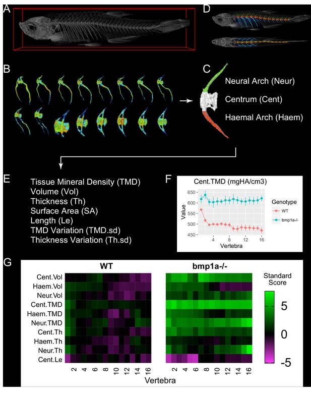
MicroCT-based phenomics in the axial skeleton of adult zebrafish.
(A) MicroCT scans are acquired in adult fish (image shows 3D volume rendering). (B) For segmentation, individual vertebrae are isolated using FishCuT (image shows 16 vertebrae from the same fish, colors indicate local thickness), and (C) each vertebral body is segmented into three skeletal elements: the Neural Arch (green), Centrum (white), and Haemal Arch/Pleural Ribs (red). A representative segmentation can be seen in (D), which depicts the same fish in (A) with an alternating color scheme used to highlight individual skeletal elements segmented by FishCuT (top: lateral view; bottom: anteroposterior view). (E) For each skeletal element, FishCuT computes the following: Tissue Mineral Density, Volume, Thickness, Surface Area, Length (centrum only), Tissue Mineral Density Variation, and Thickness Variation. (F) For analysis, each combination of element/outcome is computed as a function of vertebra number, and subjected to the global test. Shown is a plot of one combination of element/outcomes, Cent.TMD, as a function of vertebra number in WT vs. bmp1a-/- fish. (G) Standard scores are computed and arranged into ‘skeletal barcodes’ that facilitate visualization of phenotypic trends both within individuals and across groups. Shown are the skeletal barcodes for a single WT (left) and bmp1a-/- fish (right).
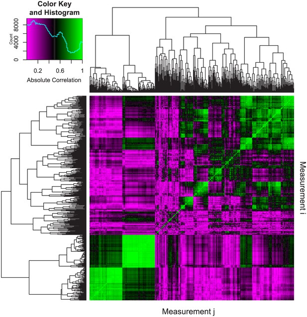
Pairwise correlations of phenotypic measurements.
The following procedure was used to assess the correlation between phenotypic measurements. First, we analyzed 34 different WT and mutant fish of various genotypes. As detailed in the text, analyzing 24 vertebrae results in 24 × 25 = 600 phenotypic measures for each fish. We denote measure i in fish n as xin (i = 1 to 600 and n = 1 to 34). Next, we computed absolute Pearson correlation coefficients between each pair of measurements as |ρi,j|=|cov(Xi,Xj)/(σ(Xi)σ(Xj))| where Xi=[xi1, xi2,...,xi34], Xj=[xj1, xj2,...,xj34], cov is the covariance, and σ is the standard deviation. The resulting 600 × 600 correlation matrix was plotted as a heatmap, where the element in the ith row and jth column represents the absolute Pearson correlation between measurement i (Xi) and measurement j (Xj). For each pairwise correlation, if a fish had missing values (e.g., not all 24 vertebrae were analyzed), it was excluded from the analysis. Hierarchical clustering was used to order the measurements in order to facilitate visualization. The predominance of purple regions indicates the prevalence of measurement pairs that exhibit low correlation. The legend depicts a color scale and a histogram of absolute correlations (computed from 600 × 600 = 360,000 different pairwise correlations). The median value of this distribution was 0.34.
-
Figure 2—source data 1
Zip file containing phenotypic data (one text file per fish) as well as R code used for analysis.
For each text file, each row represents a different vertebra, and each column represents a different phenotypic measure. The measures and their abbreviations are as follows: Tot.Vol (VertebralVolumes), Cent.Vol (CentrumVolumes), Haem.Vol (HaemalVolumes), Neur.Vol (NeuralVolumes), Tot.SA (VertebralSAs), Cent.SA (CentrumSAs), Haem.SA (HaemalSAs), Neur.SA (NeuralSAs), Tot.TMD (VertebralTMDs), Cent.TMD (CentrumTMDs), Haem.TMD (HaemalTMDs), Neur.TMD (NeuralTMDs), Tot.TMD.sd (VertebralISs), Cent.TMD.sd (CentrumISs), Haem.TMD.sd (HaemalISs), Neur.TMD.sd (NeuralISs), Tot.Th (VertebralMTs), Cent.Th (CentrumMTs), Haem.Th (HaemalMTs), Neur.Th (NeuralMTs), Tot.Th.sd (VertebralTSs), Cent.Th.sd (CentrumTSs), Haem.Th.sd (HaemalTSs), Neur.Th.sd (NeuralTSs), Cent.Le (CentrumLength).
- https://doi.org/10.7554/eLife.26014.005
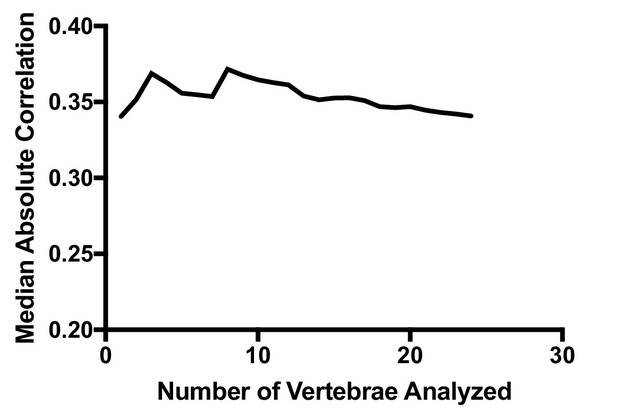
Median absolute correlation plotted as a function of number of vertebrae analyzed.
The median absolute correlation was relatively invariant with increasing number of vertebrae used for analysis.
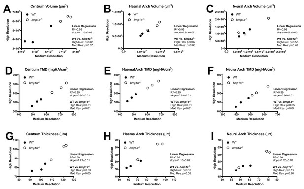
Analysis of WT and bmp1a-/- mutant fish reveals high correlation in phenotypic measurements quantified via medium and high resolution microCT.
Results are shown for the second pre-caudal vertebrae for nine different measurements (A–I). Each point represents a single animal, with the corresponding measurement assessed at two nominal isotropic resolutions: medium (21 µm voxel size) and high (10.5 µm voxel size). WT animals (n = 3) are depicted as closed circles and bmp1a-/- fish (n = 3) as open circles. Linear regressions revealed a high level of correlation. Further, t-tests showed similar p-values when comparing WT vs bmp1a-/- at each resolution.
-
Figure 3—source data 1
Zip file containing phenotypic data (one text file per fish) as well as R code used for analysis.
See legend for Figure 2—source data 1 for a listing of phenotypic measures and their abbreviations.
- https://doi.org/10.7554/eLife.26014.009
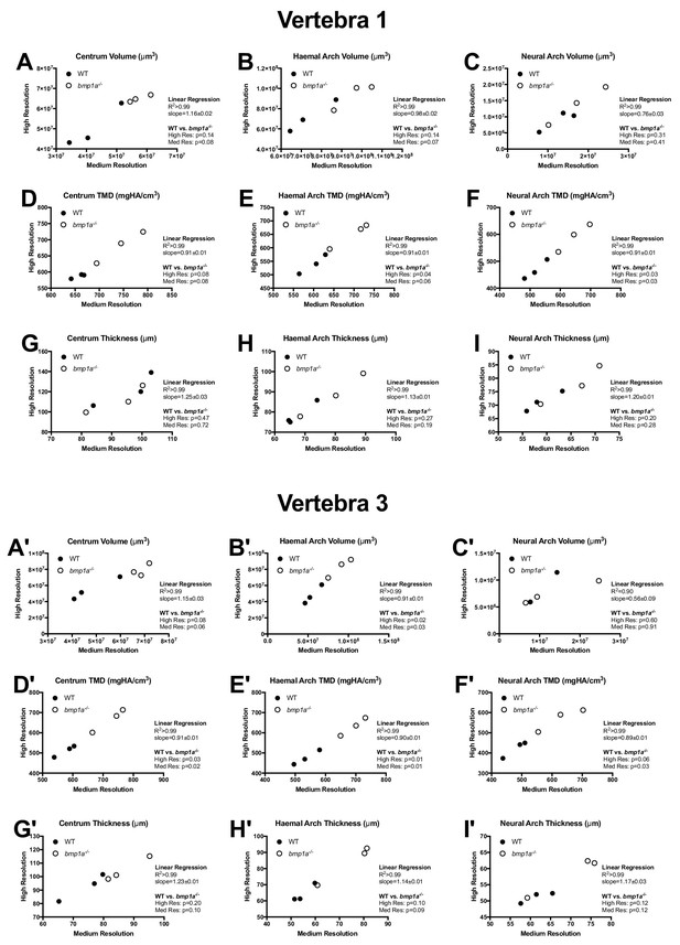
Phenotypic measurements quantified via medium and high resolution microCT scans for the first (A–I) and third (A'–I') pre-caudal vertebrae.
https://doi.org/10.7554/eLife.26014.007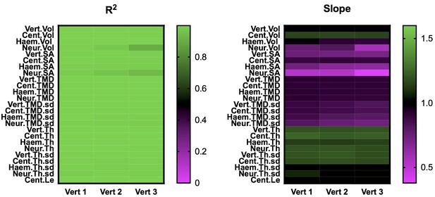
Heatmaps summarizing results from linear regressions in Figure 3 (Vert 2) and Figure 3—figure supplement 1 (Verts 1 and 3), with all phenotypic measurements reported.
https://doi.org/10.7554/eLife.26014.008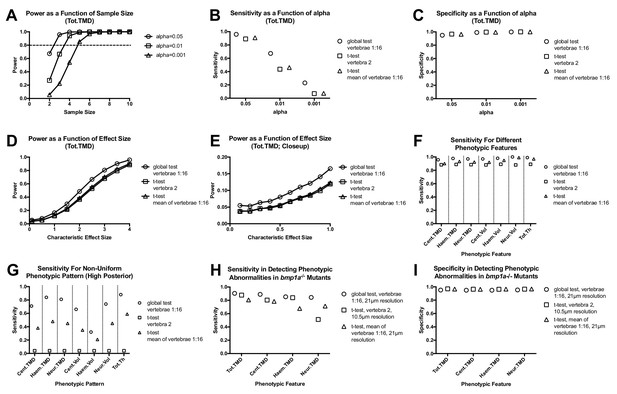
Analyzing vertebral patterns confers heightened sensitivity in discriminating mutant phenotypes compared to analyzing individual vertebrae.
Figures A-G show results from Monte Carlo simulations using simulated mutant phenotypes. (A) Power of the global test in discriminating a uniform increase in Tot.TMD (characteristic effect size: d = 4) as a function of sample size and alpha value. The dotted line highlights sample sizes with power >0.8. (B) Sensitivity (fraction of times in which p<0.05 when comparing simulated mutant vs. WT fish) for different test procedures. (C) Specificity (1 - fraction of times in which p<0.05 when comparing WT vs. WT fish) for different test procedures. (D) Power as a function effect size for different test procedures (sample size: n = 3; alpha = 0.05). (E) Closeup of figure (D) for smaller effect sizes. (F) Comparison of sensitivity for different phenotypic features (characteristic effect size: d = 4; sample size: n = 3; alpha = 0.05). (G) Sensitivity for non-uniform phenotypic pattern (linear increase from d = 0 at vert 1 to d = 4 at vert 16; n = 3; alpha = 0.05). Figure H-I show results from Monte Carlo simulations using parameter estimates derived from bmp1a-/- mutants. (H) Sensitivity in discriminating different phenotypic features in bmp1a-/- mutants. T-tests using individual vertebrae were performed on data derived from fish scanned at high resolution. (I) Specificity in discriminating different phenotypic features in bmp1a-/- mutants.
-
Figure 4—source data 1
Zip file containing phenotypic data (one text file per fish) as well as R code used for analysis.
See legend for Figure 2—source data 1 for a listing of phenotypic measures and their abbreviations.
- https://doi.org/10.7554/eLife.26014.011
-
Figure 4—source data 2
Summary of Royston test results.
For these studies we tested two subsets of 8 vertebrae (Group A: Vert 1, 3, 5, 7, 9, 11, 13, and 15; Group B: and Vert 2, 4, 6, 8, 10, 12, 14, and 16). Cent.Th, Neur.Th, Haem.Th.sd, and Cent.Le were all associated with p<0.05 for one or both groups, and thus these phenotypic features were excluded from Monte Carlo simulations.
- https://doi.org/10.7554/eLife.26014.012
-
Figure 4—source data 3
Summary of sensitivity and specificity for different test procedures.
The top table shows results assuming each phenotypic feature is uniformly elevated in simulated mutants (characteristic effect size: d = 4; sample size: n = 3; alpha = 0.05). The bottom table shows results assuming a non-uniform elevation, with the characteristic effect size linearly increasing from d = 0 at vert 1 to d = 4 at vert 16.
- https://doi.org/10.7554/eLife.26014.013
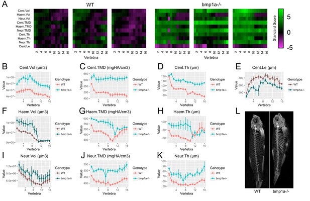
Analysis of bmp1a-/- fish.
(A) Skeletal barcodes for WT and bmp1a-/- fish (n = 3/group). Each barcode represents a single fish. Standard scores are computed as the difference between the value of the feature in the individual and the mean value of the feature across all vertebrae in the control population, divided by the standard deviation of the feature across all vertebrae in the control population (see text for details). (B–K) Phenotypic features plotted as a function of vertebra (mean ± SE, n = 3/group). Plots associated with a significant difference are colored in a lighter coloring scheme (see text for p-values). The same plots with y axis set to zero are shown in Figure 5—figure supplement 2. (L) Maximum intensity projection of microCT scans.
-
Figure 5—source data 1
Zip file containing phenotypic data (one text file per fish) as well as R code used for analysis.
See legend for Figure 2—source data 1 for a listing of phenotypic measures and their abbreviations.
- https://doi.org/10.7554/eLife.26014.017
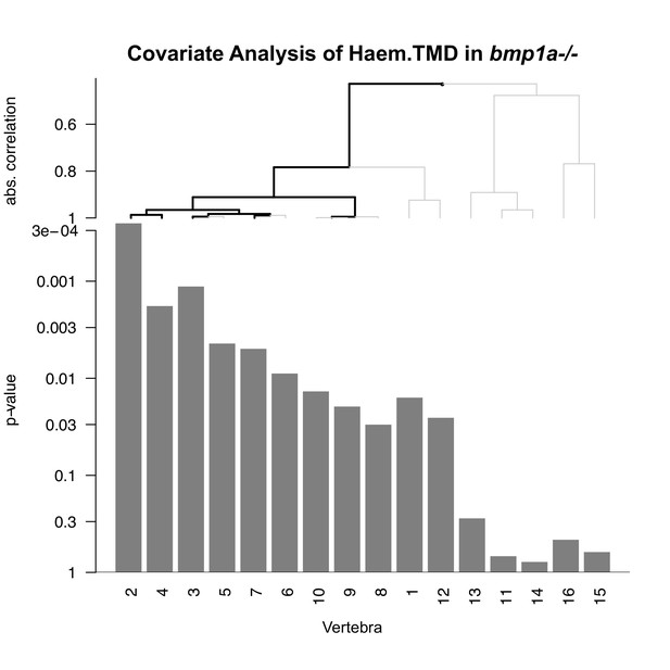
Covariate analysis of Haem.TMD in bmp1a-/- fish.
Vertebrae were hierarchically clustered based on association with mutation, and a multiplicity-corrected procedure was used to identify portions of the graph that exhibit a significant association with mutation (highlighted in black). Significant associations are observed for vertebrae 2, 3, 4, and 7. For vertebrae 9/10 significant branches did not reach all the way to the ‘leaf nodes’; in this case, we are able to infer that at least one of the vertebrae 9 or 10 was significantly associated with genotype, but not which one.
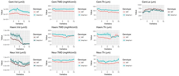
Same data as in Figure 5B–5K with y axes set to zero.
https://doi.org/10.7554/eLife.26014.016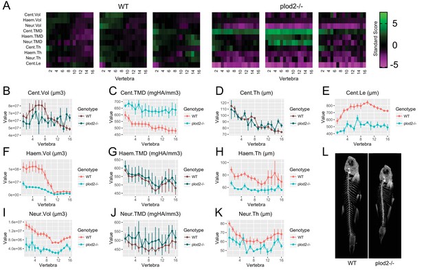
Analysis of plod2-/- fish.
(A) Skeletal barcodes for WT and plod2-/- fish (n = 3/group). WT fish in this figure are different from those in Figure 5. (B–K) Phenotypic features plotted as a function of vertebra (mean ±SE, n = 3/group). Plots associated with a significant difference are colored in a lighter coloring scheme (see text for p-values). The same plots with y axis set to zero are shown in Figure 6—figure supplement 1. (L) Maximum intensity projection of microCT scans.
-
Figure 6—source data 1
Zip file containing phenotypic data (one text file per fish) as well as R code used for analysis.
See legend for Figure 2—source data 1 for a listing of phenotypic measures and their abbreviations.
- https://doi.org/10.7554/eLife.26014.020
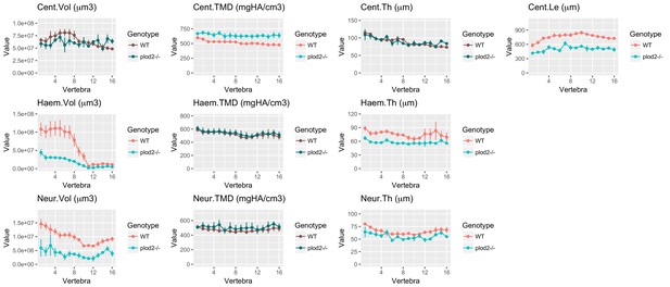
Same data as in Figure 6B–6K with y axes set to zero.
https://doi.org/10.7554/eLife.26014.019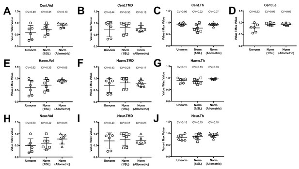
Allometric normalization for differences in body size.
Data are shown for the first precaudal vertebra of n = 6 WT fish of different standard lengths. The coefficient of variability (CV) is shown for each normalization procedure. The left column shows high phenotypic variability in unnormalized data. When data were normalized using allometric models (right column), phenotypic variability was substantially reduced. Phenotypic variability was also reduced, though to a lesser extent, when data were normalized using an alternate normalization, 1/SL (middle column).
-
Figure 7—source data 1
Zip file containing phenotypic data (one text file per fish) as well as R code used for analysis.
See legend for Figure 2—source data 1 for a listing of phenotypic measures and their abbreviations.
- https://doi.org/10.7554/eLife.26014.024
-
Figure 7—source data 2
Summary of scaling exponents (i.e., values of b) computed in allometric models.
Expected values for isometric scaling with standard length are as follows: Vol: b = 3, TMC: b = 3, Th: b = 1, Le: b = 1.
- https://doi.org/10.7554/eLife.26014.025
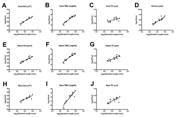
Allometric modeling of phenotypic features.
Phenotypic features (data are shown for the first precaudal vertebra) plotted as a function of standard length. Linear fits of log-transformed data were used to compute allometric model parameters.
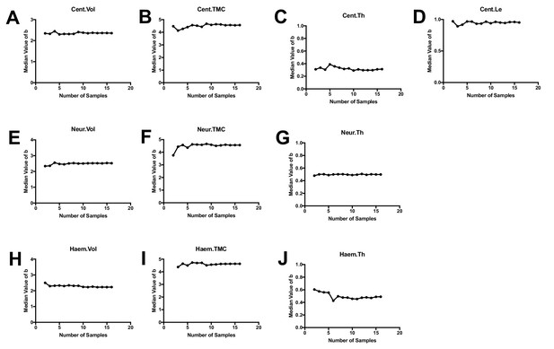
Convergence analysis for allometric modeling.
Plots show the computed value of the scaling exponent b when a subset of samples of a specified sample size was selected from our group of n = 16 animals (values are median values from multiple simulations for each sample size). For each phenotypic feature, the median value of b stabilizes for sample sizes greater than ~5–10.
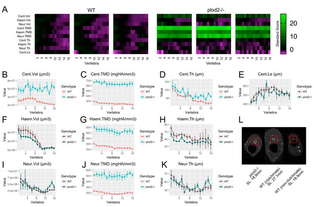
Analysis of plod2-/- fish following removal of allometric effects of body size.
(A) Skeletal barcodes for WT and plod2-/- fish following removal of allometric effects of body size (n = 3/group). (B–K) Phenotypic features as a function of vertebra (mean ± SE, n = 3/group). Phenotypic data in WT sibling controls were subjected to allometric normalization; data in plod2-/- fish are identical to those in Figure 6. Plots associated with a significant difference are colored in a lighter coloring scheme (see text for p-values). Values for TMD were derived by a two-step process in which TMC and volume were subjected to allometric normalization independently, and normalized values for TMC and volume were used to calculate normalized values for TMD. The same plots with y axis set to zero are shown in Figure 8—figure supplement 1. (L) Transverse sections of microCT scans. Centra are highlighted by a red box in each animal. plod2-/- mutants (left) exhibit increased centrum diameter compared to standard length matched, non-clutchmate WT controls (right), and to a lesser extent, WT siblings (middle) of greater standard length. Images show posterior endplate of the sixth precaudal vertebra in all fish.
-
Figure 8—source data 1
Zip file containing phenotypic data (one text file per fish) as well as R code used for analysis.
See legend for Figure 2—source data 1 for a listing of phenotypic measures and their abbreviations.
- https://doi.org/10.7554/eLife.26014.028
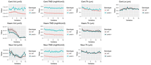
Same data as in Figure 8B–8K with y axes set to zero.
https://doi.org/10.7554/eLife.26014.027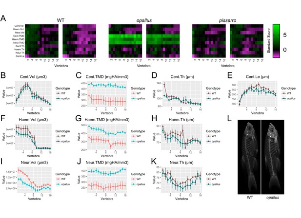
Identification of opallus as a novel axial skeletal mutant.
(A) Skeletal barcodes for WT, opallus, and pissarro (n = 2 fish/group). Barcodes for opallus, but not pissarro, appear different from WT fish (B–K) Phenotypic features in opallus plotted as a function of vertebra (mean ±SE, n = 5/group). Plots associated with a significant difference are colored in a lighter coloring scheme (see text for p-values). The same plots with y axis set to zero are shown in Figure 9—figure supplement 2. (L) Maximum intensity projections of microCT scans.
-
Figure 9—source data 1
Zip file containing phenotypic data (one text file per fish) as well as R code used for analysis.
See legend for Figure 2—source data 1 for a listing of phenotypic measures and their abbreviations.
- https://doi.org/10.7554/eLife.26014.032
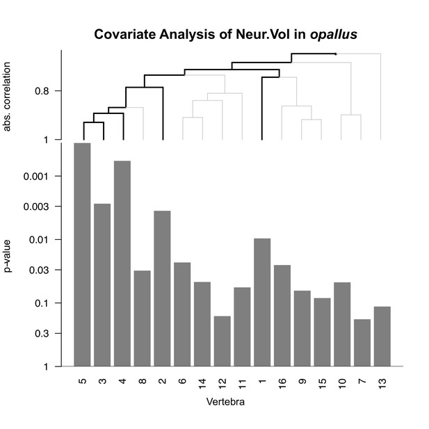
Covariate analysis of Neur.Vol in opallus.
See Figure 5—figure supplement 1 for interpretation of graph. Significant associations are observed for vertebrae 1–5 only.
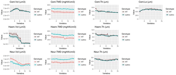
Same data as in Figure 9B–K with y axes set to zero.
https://doi.org/10.7554/eLife.26014.031Additional files
-
Transparent reporting form
- https://doi.org/10.7554/eLife.26014.033


