T2N as a new tool for robust electrophysiological modeling demonstrated for mature and adult-born dentate granule cells
- Ernst Strüngmann Institute (ESI) for Neuroscience in Cooperation with Max Planck Society, Germany
- Frankfurt Institute for Advanced Studies, Germany
- Goethe University, Germany
- Universidad Nacional del Comahue-CONICET, Argentina
Figures
Figure 1
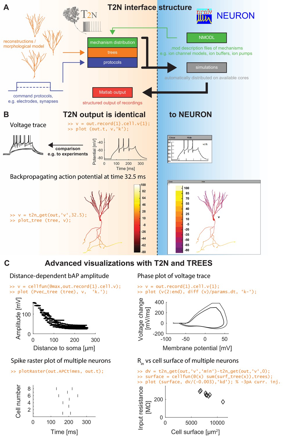
TREES-to-NEURON (T2N) interface linking compartmental modeling environment NEURON with morphology modeling and analysis tools of Matlab and TREES toolbox.
T2N enables fast and simple incorporation of many diverse morphologies in compartmental simulations facilitating the search for morphologically robust biophysical models. (A) Illustration of T2N workflow. T2N allows for setting up a full compartmental model in Matlab by importing reconstructed or synthetic morphologies (orange; e.g. from NeuroMorpho.org) and by distributing subcellular channel mechanisms (green; mod files generated with NEURON’s NMODL or obtained from databases such as IonChannelGenealogy or Channelpedia). In addition, T2N enables setting up full simulation control by attaching stimulation and recording electrodes and specifying simulation conditions (e.g. stimulation protocols; blue). T2N then automatically produces stereotyped NEURON hoc code, initializes and runs simulations and returns recorded data in a structured output format (red). (B) A comparison of two example results in NEURON and T2N validates T2N simulation output. The orange script shows sample code for visualizing the output. Upper row: somatic voltage trace during a current injection. Lower row: membrane voltage at each dendrite location at a single time point. (C) Examples of using T2N for a simple and fast analysis and visualization of simulation results. (Code for creating the panels is shown in orange; code for the specific labels is omitted).
Figure 2
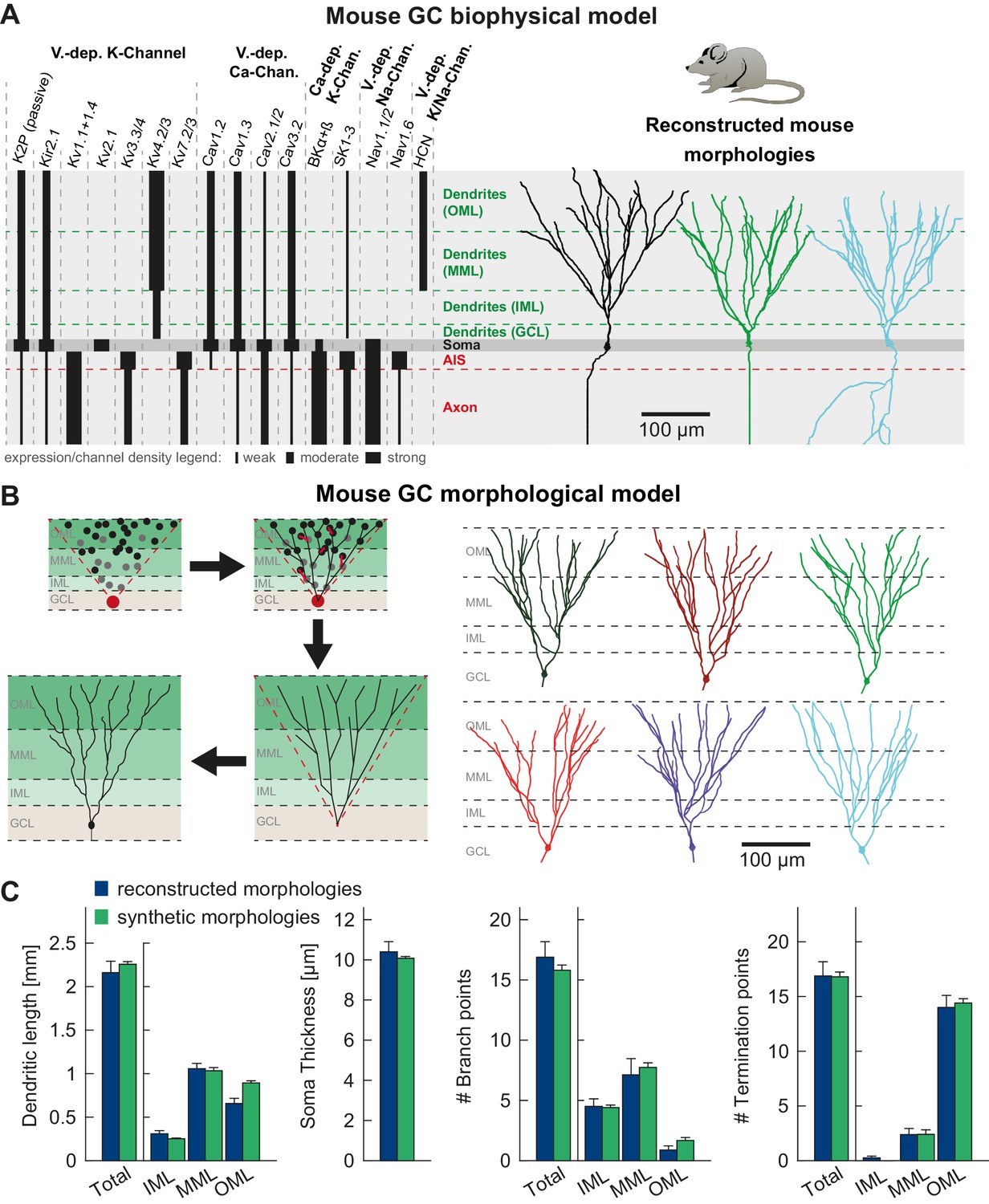
T2N supports incorporation of realistic ion channels and synthetic morphologies.
(A) Ion channel composition of the mouse dentate granule cell (GC) model. Left: Passive and active ion channels with their specific distribution in six different regions: outer molecular layer (OML), middle molecular layer (MML), inner molecular layer (IML), soma, axon initial segment (AIS) and axon. The relative spatial distribution of voltage-dependent (V.-dep.) and calcium-dependent (Ca2+-dep.) channels is in line with an extensive amount of data from the literature (see Table 1, Appendix 2 and Materials and methods for details). Right: Three exemplary morphologies out of eight reconstructed mouse GCs (Schmidt-Hieber et al., 2007) used for compartmental modeling of mouse GCs. (B) Schematic of the morphological model used to generate synthetic mouse morphologies which is analogous to the previously reported rat model (Beining et al., 2017; see Material and methods there for details). Upper left: A synthetic 3D young dentate gyrus (DG) was created comprising different layers (GCL, IML, MML, and OML, from bottom to top). A soma (red dot) was defined and random target points (black dots) were distributed within a 3D cone (red dashed lines). These points were complemented by directed target points (gray dots) that were placed automatically between clusters of target points and the soma. Upper right: The target points were connected by a minimum spanning tree algorithm (Cuntz et al., 2010) and terminal dendritic segments shorter than 20 µm were pruned off (red segments, see Beining et al., 2017). Lower right: The young DG and the dendritic tree have been stretched to their mature size (see Beining et al., 2017 for more information). Lower left: Adding a somatic diameter profile, a synthetic axon, applying jittering and dendritic diameter taper (not shown for visualization purposes) to the dendrites results in realistic synthetic GC morphologies suitable for compartmental modeling. (C) Six out of 15 synthetic morphologies created by the morphological model and used for compartmental modeling with their anatomical borders (gray dashed lines). (D) General and layer-specific structural comparison of the reconstructed (blue, Schmidt-Hieber et al., 2007) and synthetic (green) mouse GC morphologies.
Figure 3 with 4 supplements
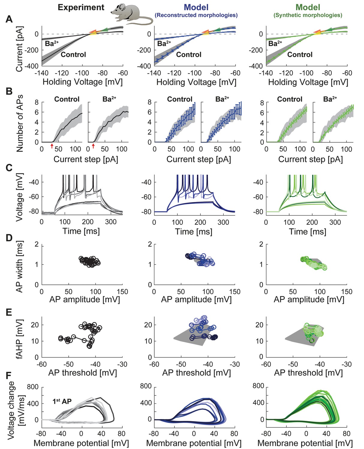
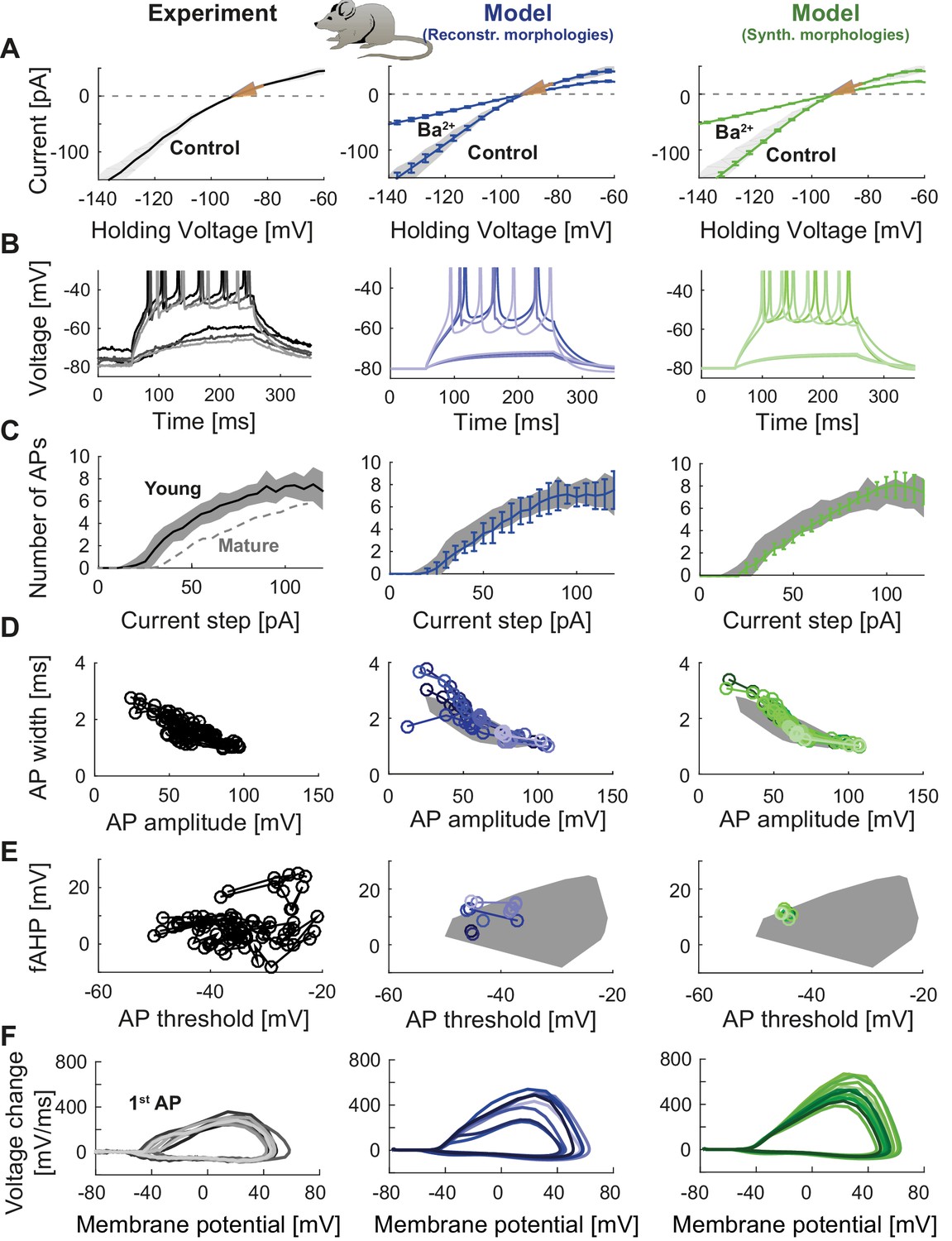
Passive and active properties of the mature mouse GC model.
Comparison of electrophysiological features between experimental data (left column, grayish colors) (Mongiat et al., 2009), GC model with reconstructed morphologies (middle column, blueish colors) and GC model with synthetic morphologies (right column, greenish colors). (A) Current-voltage (I–V) relationships before and after application of 200 µM Ba2+. Simulations (blue and green curves) are compared to experimental data (mean and s.e.m. from raw traces (Mongiat et al., 2009) as black curve and gray patch; arrows are average values reported from further literature: red (Brenner et al., 2005), yellow (Mongiat et al., 2009), green (Schmidt-Hieber et al., 2007)). Ba2+ simulations correspond to 99% Kir2 and 30 % K2P channel blockade. (B) Number of spikes elicited by 200 ms current steps (F-I relationship) from a holding potential of −80 mV. Right subgraph shows F-I relation after adding Ba2+. Experimental standard deviation is shown as gray patches in all columns. Red arrows point to the rheobase, which is different between control and BaCl2 application. (C) Exemplary spiking traces from control condition in (B) (200 ms, 30 and 75 pA somatic current injections). (D–E) Action potential (AP) features of the first AP (90 pA somatic step current injection, 200 ms). Convex hulls around experimental data are shown in all columns as gray patches. (D) AP width vs. AP amplitude. (E) Amplitude of fast afterhyperpolarisation (fAHP) vs. AP threshold. (F) Phase plots of the first AP (dV/V curve, 90 pA current step, 200 ms).
Figure 3—figure supplement 1
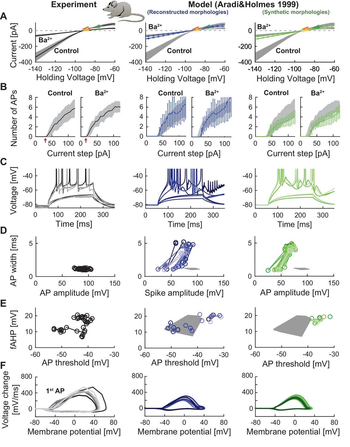
Performance of a widely used GC model with reconstructed and synthetic mouse morphologies.
This figure is analogous to Figure 3 (experimental data in left column, grayish colors) but in order to compare our model’s robustness to standard mature GC models, the biophysical model of Aradi and Holmes (Aradi and Holmes, 1999) was used here together with our set of reconstructed (middle column, blueish colors) and synthetic (right column, greenish colors) mouse morphologies. (A) Current-voltage (I–V) relationships before and after application of 200 µM Ba2+. Simulations (blue and green curves) are compared to experimental data (mean and s.e.m. from raw traces (Mongiat et al., 2009) as black curve and gray patch; arrows are average values reported from further literature: red (Brenner et al., 2005), yellow (Mongiat et al., 2009), green (Schmidt-Hieber et al., 2007)). Ba2+ simulations here only correspond to 30% passive channel blockade as this model does not include Kir2 channels. (B) Number of spikes elicited by 200 ms current steps (F-I relationship) including Ba2+ block as in A). Experimental standard deviation is shown as gray patches in all columns. (C) Exemplary spiking traces (200 ms, 30 and 90 pA somatic current injections. This is different to Figure 3 because no spiking occurred at 75 pA in the Aradi and Holmes mature GC model. (D–E) Action potential (AP) features of the first AP (90 pA somatic step current injection, 200 ms). Convex hulls around experimental data are shown in all columns as gray patches. (D) AP width vs. AP amplitude. (E) Amplitude of fast afterhyperpolarisation (fAHP) vs. AP threshold. (F) Phase plots of the first AP (dV/V curve, 90 pA current step, 200 ms).
Figure 3—figure supplement 2
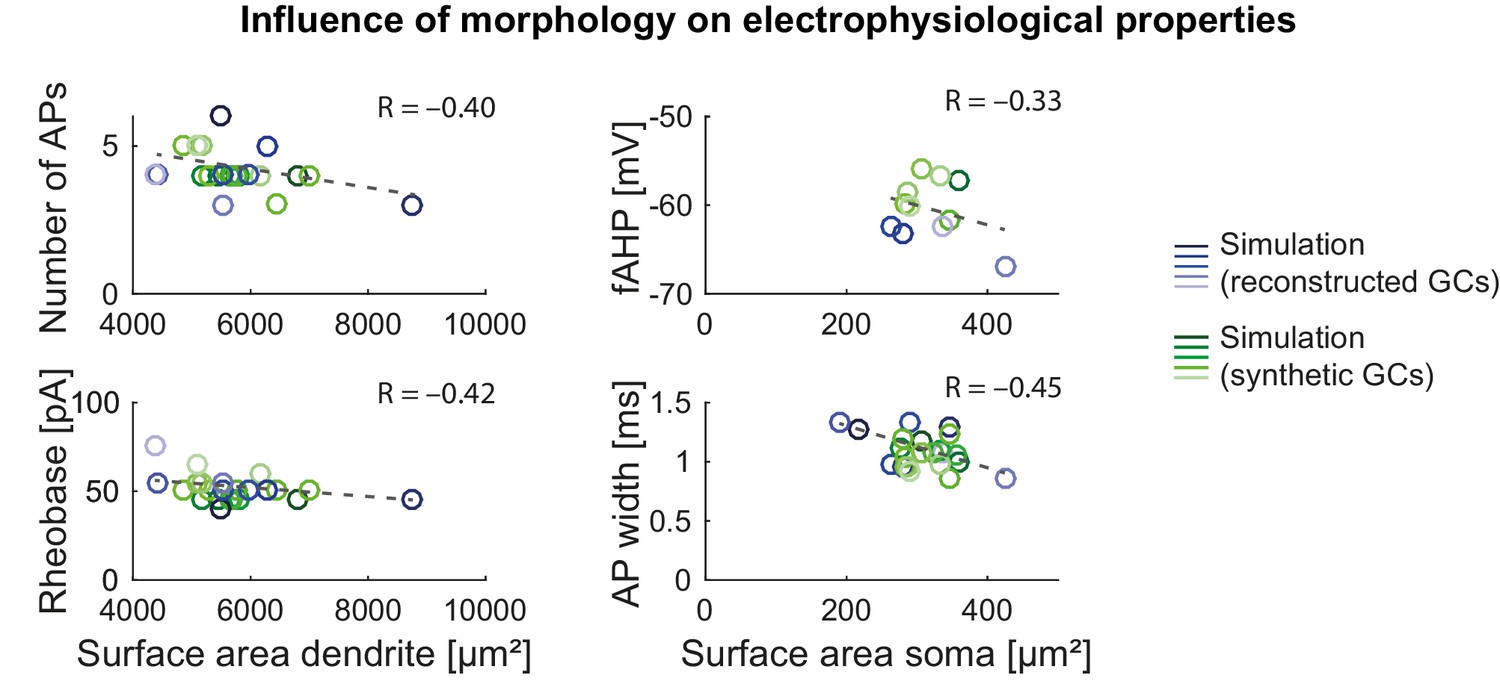
Influence of morphology on electrophysiological properties in the mature mouse GC model.
Influence of dendritic (left column) and somatic (right column) surface size on electrophysiological parameters (fAHP, AP width, AP threshold and number of APs) in the model with reconstructed (blue circles) and synthetic (green circles) morphologies. Correlation coefficients are given as inset text and trend lines are shown as gray dashed lines.
Figure 3—figure supplement 3
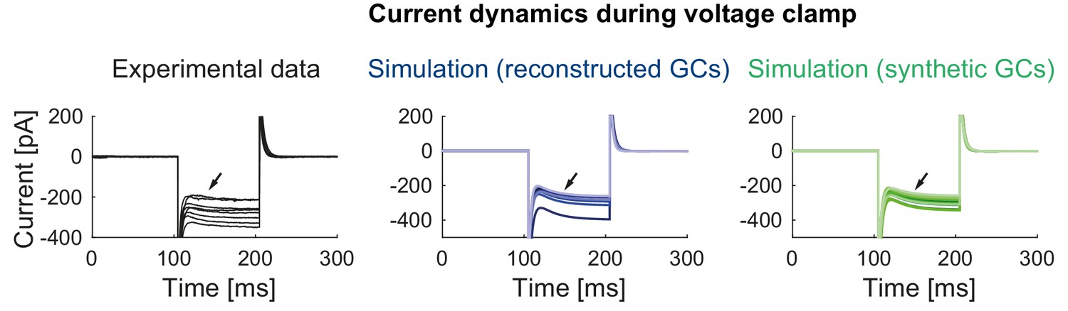
Current dynamics during voltage clamp in mature mice GCs.
Currents measured during a highly hyperpolarized voltage step (−120 mV) in the experiment (left) and the models with reconstructed (middle) and synthetic (right) morphologies. The slowly activating currents (black arrows) originate from Kir currents in the model.
Figure 3—figure supplement 4
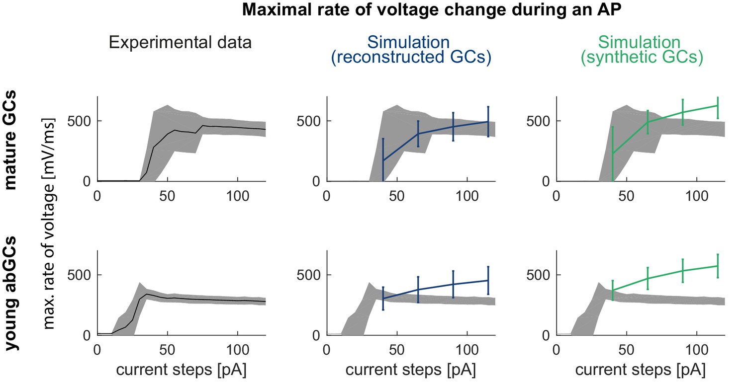
Maximal rate of voltage change during an AP in the mature mouse GC model.
The maximal voltage deflection during a spike shows a sudden jump and then slow decay in the experiment when current amplitudes are increased in mature (upper row, left) and young GCs (lower row, left) which is not reproduced in the mature/young GC model with the na8st sodium channel model (from Schmidt-Hieber and Bischofberger, 2010) in reconstructed (middle column) or synthetic (right column) morphologies.
Figure 4 with 1 supplement

Mature rat GC model.
Comparison of electrophysiological features between GC model with reconstructed morphologies (left column, blueish colors) and GC model with synthetic morphologies (right column, greenish colors) as it was adapted for reproducing rat data. (A) Illustration of reconstructed (left) and synthetic (right) rat morphologies used for simulations of rat GCs, from (Beining et al., 2017). (B) I-V relationship of the model with (dark solid lines) or without (bright dashed lines) adjustment of passive conductance to experimental rat data (indicated by arrows: red (Staley et al., 1992), yellow (Mateos-Aparicio et al., 2014), green (Pourbadie et al., 2015), violet (Schmidt-Hieber et al., 2004). (C) F-I relationship of the model compared to data (black line and standard deviation as gray patch) from Pourbadie et al., 2015. (D) Exemplary spiking traces simulated during a 1 s current injection of 200 pA.
Figure 4—figure supplement 1
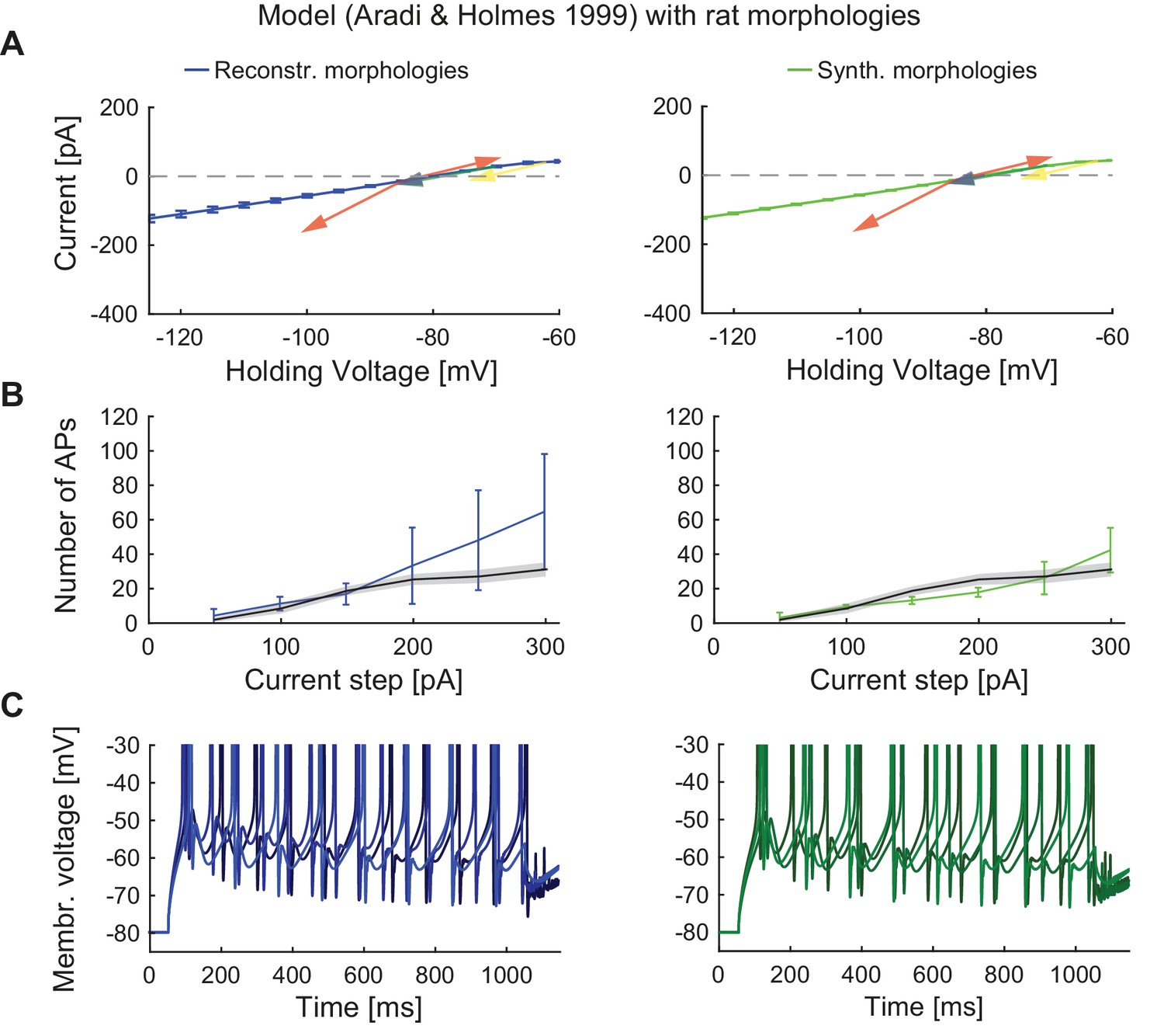
Performance of the classical GC model with reconstructed and synthetic rat morphologies.
This figure is analogous to Figure 4 but in order to compare our model’s robustness to standard GC models, the biophysical model of Aradi and Holmes (Aradi and Holmes, 1999) was used here with reconstructed (middle column, blueish colors) and synthetic (right column, greenish colors) rat morphologies. (A) I-V relationship of the model (dark solid lines) compared to experimental rat data (indicated by arrows: red (Staley et al., 1992), yellow (Mateos-Aparicio et al., 2014), green (Pourbadie et al., 2015), and violet (Schmidt-Hieber et al., 2004). (B) F-I relationship of the model compared to data (black line and standard deviation as gray patch) from (Pourbadie et al., 2015). (C) Exemplary spiking traces simulated during a 1 s current injection of 200 pA.
Figure 5 with 1 supplement
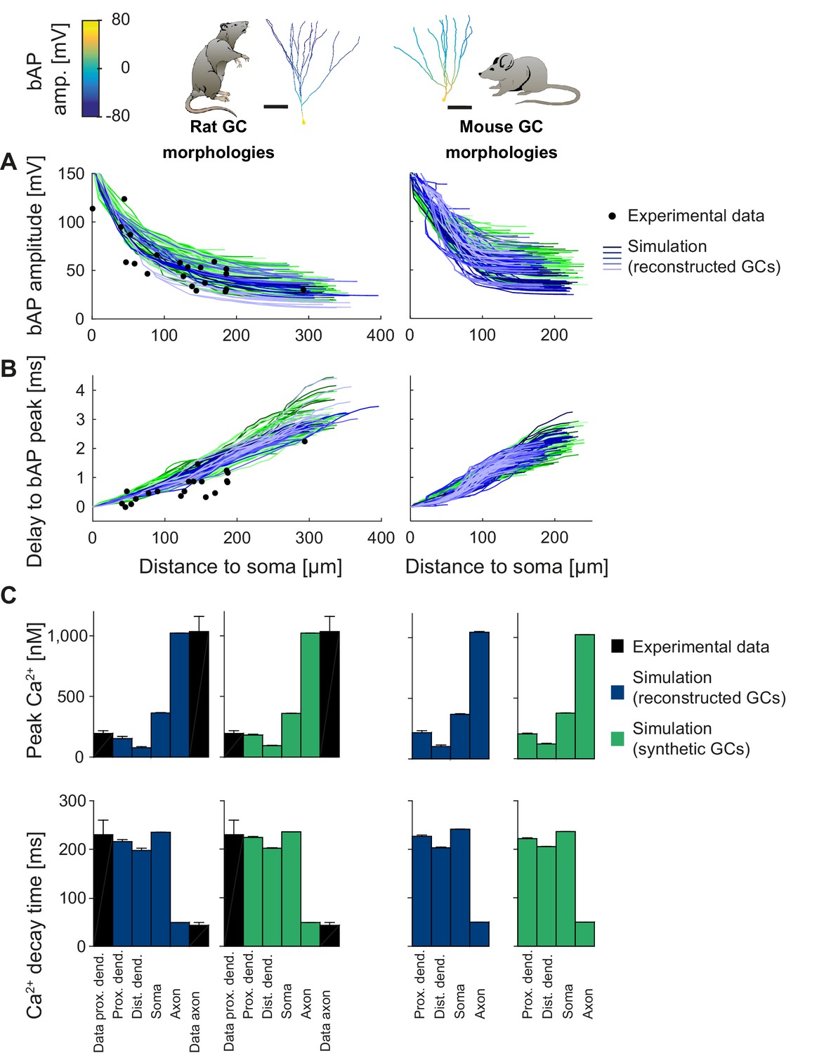
Backpropagating action potentials (bAPs) in mature mouse and rat GC models.
bAP characteristics at 33°C (experiment and simulation), elicited in the soma by a brief current injection. Inset: Exemplary rat and mouse GC morphology with local maximum voltage amplitudes. (A) Maximal voltage amplitude as a function of Euclidean distance from the soma. Black data points are experimental data from rat (Krueppel et al., 2011). There are no available data on bAP characteristics for mouse GCs. (B) Corresponding delay of the maximal bAP amplitude in the model compared to experimental rat data (black dots) (Krueppel et al., 2011). (C) Peak Ca2+ amplitudes at room temperature following an AP measured at different locations in the rat (left) and mouse (right) GC model using reconstructed (blue) and synthetic (green) morphologies. Experimental rat data measured in proximal dendrites (Stocca et al., 2008) and axonal mossy fiber boutons (MFBs) (Jackson and Redman, 2003) are added as black bars. There are no available data on bAP characteristics for mouse GCs. (D) Ca2+ decay time constants analogous to C.
Figure 5—figure supplement 1
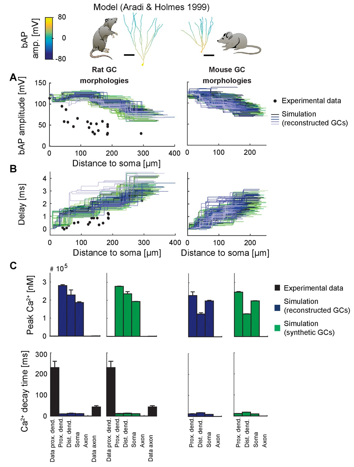
Backpropagating action potentials (bAPs) in the classical GC model.
bAP characteristics at 33°C (experiment and simulation), elicited in the soma by a brief current injection. Inset: Exemplary rat and mouse GC morphology with local maximum voltage amplitudes. Note that in order to measure dendritic bAP and Ca2+ characteristics in the classical GC model using a short strong current pulse as in Figure 5, it was necessary to isolate the cell from its axon (by increasing Ra) because the latter was a source of ongoing spike generation after the first spike in most morphologies and thus made measurements otherwise impossible. (A) Maximal voltage amplitude as a function of Euclidean distance from the soma. Note the higher amplitudes in the dendrites due to activated Nav channels there. Black data points are experimental data from rat (Krueppel et al., 2011). (B) Corresponding delay of the maximal bAP amplitude in the model compared to experimental rat data (black dots) (Krueppel et al., 2011). (C) Peak Ca2+ amplitudes at room temperature following an AP measured at different locations in the rat (left) and mouse (right) GC model using reconstructed (blue) and synthetic (green) morphologies. Note that the Aradi and Holmes mature GC model has no Ca2+ channels in the axon, thus the measurement was omitted there. Experimental rat data measured in proximal dendrites (Stocca et al., 2008) and axonal mossy fiber boutons (MFBs) (Jackson and Redman, 2003) are added as black bars, which are very small, as the Ca2+ concentrations in the Aradi and Holmes GC model are higher by a factor of ~1000 compared to our model. (D) Ca2+ decay time constants analogous to C.
Figure 6 with 2 supplements
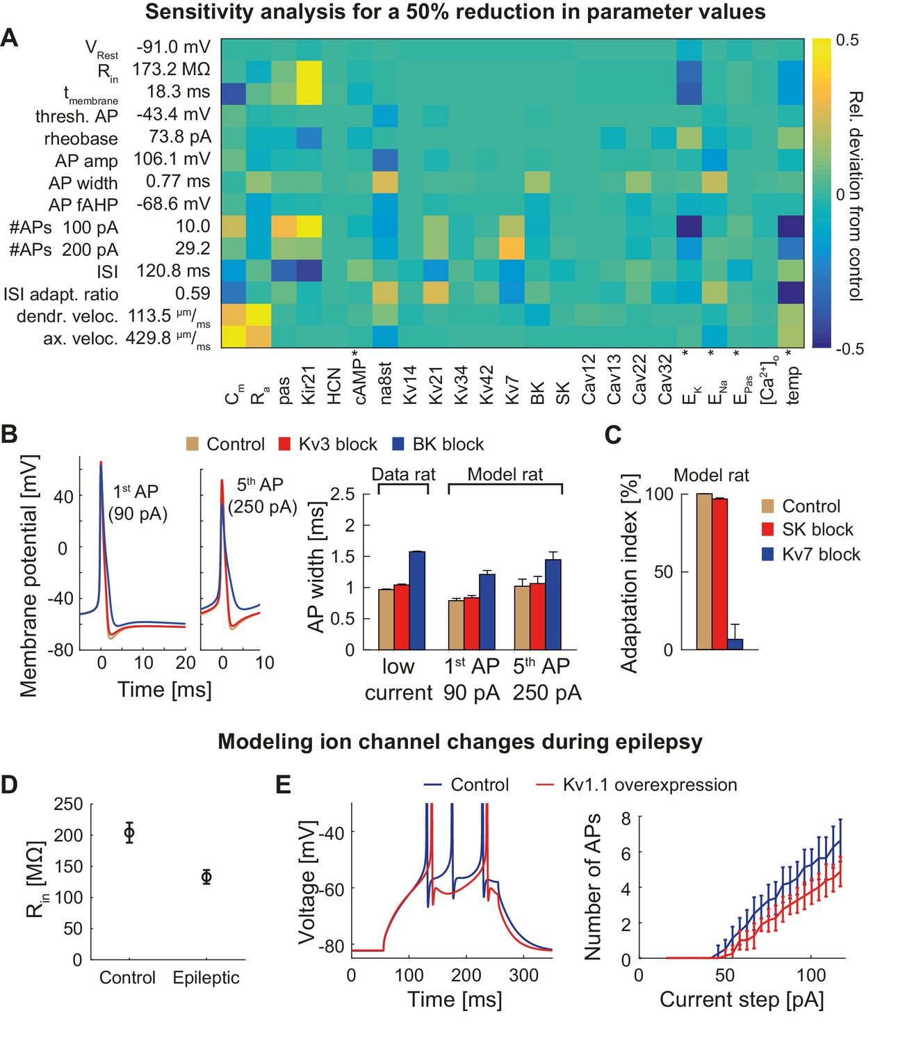
Dependence of the model on specific channels and parameters.
(A) Sensitivity matrix showing the relative change (color-coded) in electrophysiological parameters (y-axis) in the mature rat GC model following a 50% reduction in ion channel densities or other model parameters (x-axis), except for the cases marked with an asterix (*): the reversal potential of potassium EK as well as the passive reversal potential EPas were raised by +10 mV (to reduce ionic drive) and ENa was lowered by −20 mV. The temperature was raised by +10°C. cAMP concentration (influencing HCN channels in the model) was raised from 0 to 1 µM. (B) Left: Exemplary voltage traces during 1 s current injection of 90 pA (left, first AP) or 250 pA (right, fifth AP) under control (black lines), Kv3.4 block (red lines) or BK block (blue lines) conditions in the mature rat GC model. Right: Half-amplitude AP widths compared to experimental data that used paxilline to block BK (Brenner et al., 2005; Müller et al., 2007) or BDS-I to block Kv3.4 channels (Riazanski et al., 2001). (C) Impact of the blockade of SK and Kv7 channels on spike frequency adaptation in the mature rat GC model. (D) Input resistance measurements in the rat GC model in the control case and when post-epileptic conditions are modeled (doubled Kir2 and HCN channel conductance). (E) A reported overexpression of Kv1.1 following an in vivo approach to elicit temporal lobe epilepsy in mice (Kirchheim et al., 2013) was mimicked in silico by a three-fold increase of Kv1.1 channel density in the mature mouse GC model. Left graph illustrates increased spiking delay, whereas the right plot shows the reduced excitability.
Figure 6—figure supplement 1
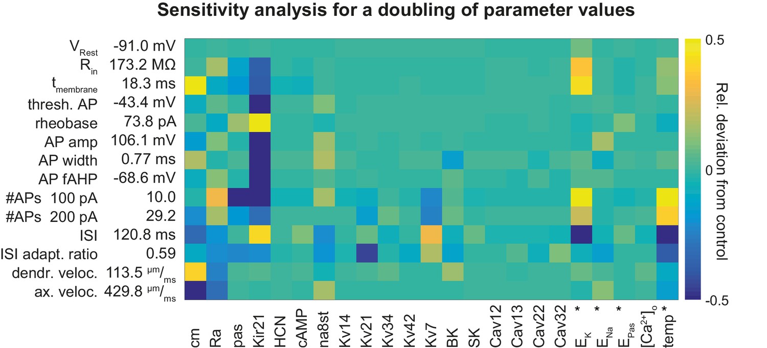
Sensitivity analysis for a doubling of parameter values in the mature rat GC model.
Sensitivity matrix analogous to Figure 6A but with increased (doubled) instead of reduced channel densities or parameters except for the cases marked with an asterix (*): the reversal potential of potassium EK was lowered by −20 mV (to increase ionic drive) and ENa was increased by +20 mV. HCN is increased from 0 to 1 µM in both cases. Temperature was reduced from 24°C to 14°C.
Figure 6—figure supplement 2
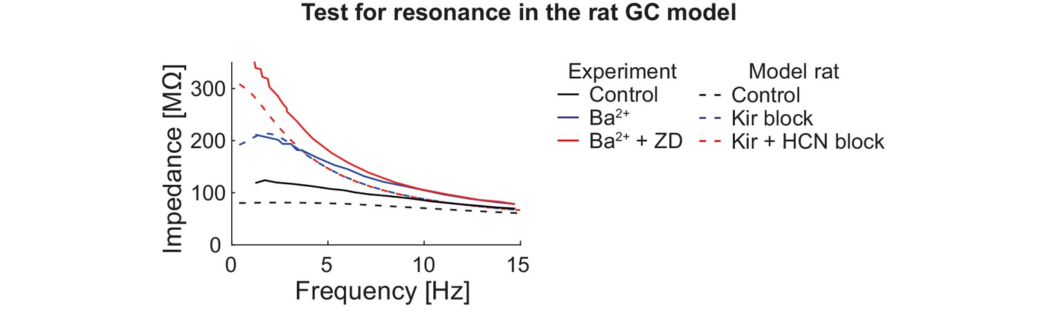
Test for resonance in the rat GC model.
GCs were injected with oscillating currents of increasing frequency to calculate their impedance. The graph shows experimental (solid curves, human GCs (Stegen et al., 2012)) and simulation (dashed curves, rat GCs) data under control conditions (black) and when Kir (blue) or Kir and HCN (red) channels are blocked.
Figure 7
Model of young adult-born granule cells (abGCs) in mice.
Panels are analogous to Figure 3, with comparison of electrophysiological features between experimental data (left column, grayish colors), GC model with reconstructed morphologies (middle column, blueish colors) and GC model with synthetic morphologies (right column, greenish colors). The experimental data of young abGCs at a cell age of 28 dpi is from Mongiat et al. (2009). The model was obtained by a reduction of several ion channels (see Table 3). (A) Current-voltage (I–V) relationships before and after application of 200 µM Ba2+; Ba2+ simulations correspond to 99% Kir2 and 30 % K2P channel blockade. Experimental measurements of Rin in 28 dpi old abGCs from further literature are indicated by arrows (red [Mongiat et al., 2009], green [Piatti et al., 2011], pink [Yang et al., 2015]). (B) Exemplary spiking traces (200 ms, 10 and 50 pA somatic current injections). (C) Number of spikes elicited by 200 ms current steps (F-I relationship). Experimental standard deviation is shown as gray patches in all columns and the F-I curve of mature GCs is plotted in the left column (gray dashed line) for comparison. (D–E) Action potential (AP) features (90 pA somatic step current injection, 200 ms). Convex hulls around experimental data are shown in all columns as gray patches. (D) AP width vs. AP amplitude. (E) Amplitude of fast afterhyperpolarisation (fAHP) vs. AP threshold. (F) Phase plots of the first AP (dV/V curve, 90 pA current step, 200 ms).
Figure 8
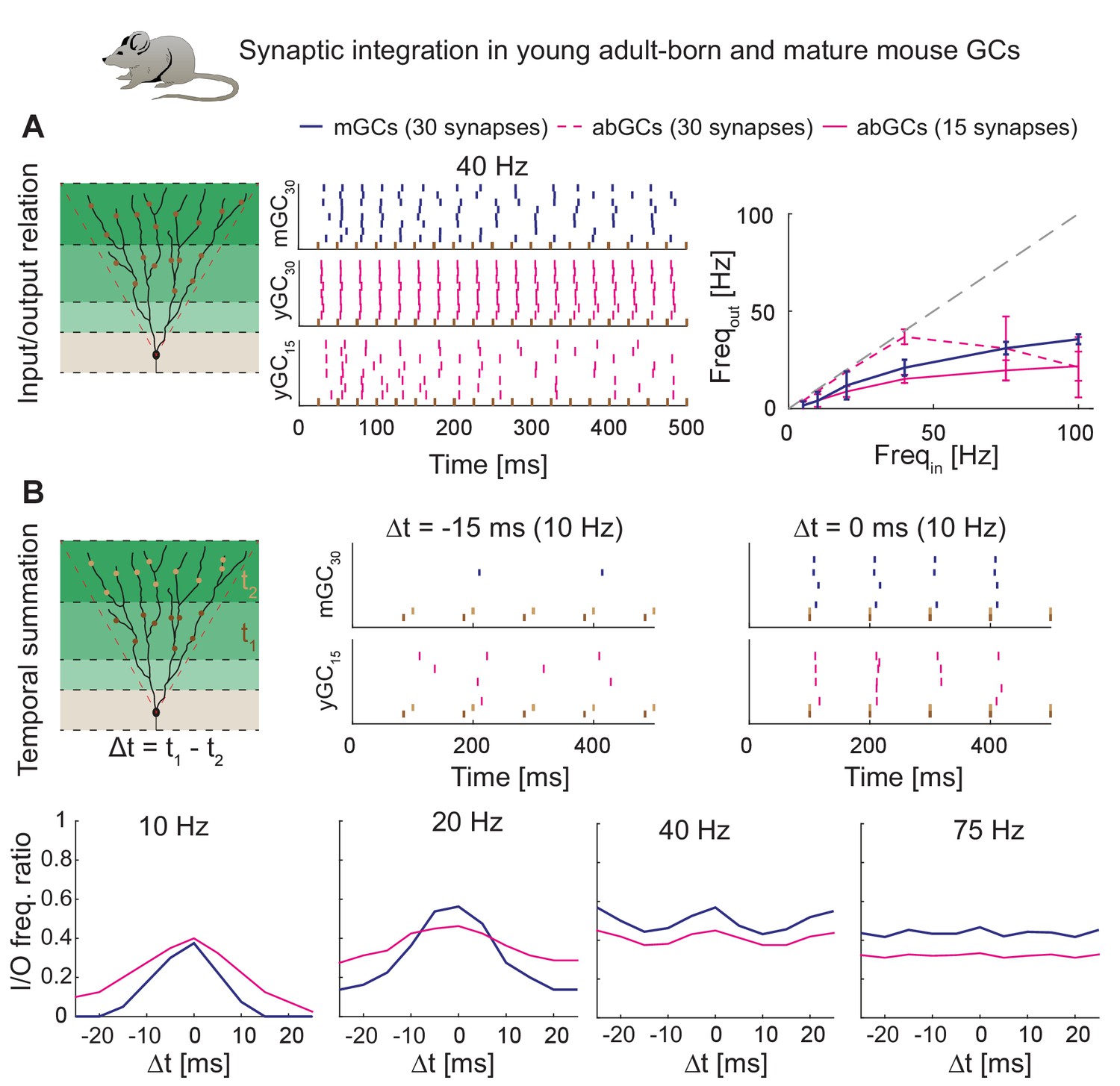
Synaptic integration in young abGCs vs. mature GCs.
(A) Left: Scheme of the simulation configuration with 15 synapses distributed in the MML and 15 in the OML. Middle: All synapses are activated synchronously at 40 Hz. Note that young abGCs (middle row) followed the input (black vertical lines) better than mature GCs (upper row), but performed similarly (lower row) when the biologically lower synapse number (15 synapses in total, yGC15) was implemented. Right: Summary of the input/output relation at all tested frequencies (5, 10, 20, 40, 75, 100 Hz). Gray dashed line illustrates the theoretically perfect input/output ratio. (B) Upper left: Scheme of the simulation configuration when MML and OML synapses are activated with a delay of Δt to analyze temporal summation of inputs. Upper right: Note that young abGCs perform better than mature GCs at following the 10 Hz input when the MML and OML inputs are delayed (left, −15 ms) compared to synchronous activation (right, 0 ms). Lower row: Summary over all tested frequencies (10, 20, 40, 75 Hz) showing that young abGCs have a broader time window of temporal summation than mature GCs at low frequencies but perform slightly worse than mature GCs at high frequencies.
Appendix 2—figure 1

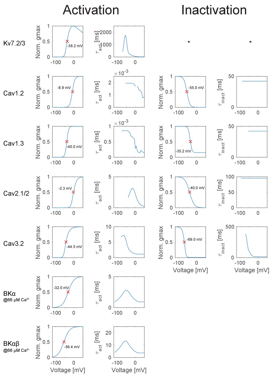
Overview of the ion channel activation and inactivation kinetics in the GC model.
The illustrated voltage-dependent kinetics were automatically calculated and plotted with a function of the T2N package, which applied voltage step protocols to a single compartment comprising only the ion channel of interest. First column: Activation curves of all ion channels used in the GC model. The red crosses denote the half-activation voltage, which is additionally inserted as text in each case. Second column: Curve of the activation time constant at different voltages obtained with a monoexponential fit to the rise in conductance. Degree symbol (°) denotes that only the fast inactivation component was fitted. Third column: Inactivation curves of all ion channels used in the GC model. The red crosses denote the half-inactivation voltage, which is additionally inserted as text in each case. Fourth column: Curve of the inactivation time constant at different voltages obtained with a monoexponential fit to the decay in conductance. Asterisk (*) denotes cases where no inactivation occurred, e.g. for the hyperpolarization-activated ion channels Kir2.x and HCN.
Appendix 2—figure 2
Overview of the ion channel activation and inactivation kinetics in the GC model (continued from Appendix 2—figure 1).
https://doi.org/10.7554/eLife.26517.026Tables
Table 1
Summary of all ion channel models and densities implemented in the mouse mature GC model.
Categorial values of the ion channel expression profiles: 0 = not existent or very weak, 1 = weak, 2 = moderate, 3 = strong. Conductances [mS/cm²] for each ion channel used in the model are given in the gray fields.
Table 2
Electrophysiology in mature mouse GCs – experiment vs. model.
https://doi.org/10.7554/eLife.26517.010| Intrinsic properties | Experiment | Model reconstr. morphologies | Model synth. morphologies |
|---|---|---|---|
| Rin [MΩ] (@ −82.1 mV) | 289.5 ± 34.9 | 287.0 ± 14.7 | 279.6 ± 6.9 |
| cm [pF] | 48.9 ± 5.3 | 55.7 ± 2.8 | 61.2 ± 1.6 |
| tau [ms] | 34.0 ± 2.0 | 31.4 ± 0.2 | 31.6 ± 0.1 |
| Vrest [mV] | −92.7 ± 0.5 * | −88.7 ± 0.1 | −88.6 ± 0.0 |
| Ithreshold [pA] | 47.5 ± 4.5 | 52.5 ± 3.7 | 50.3 ± 1.6 |
| Vthreshold [mV] | −46.3 ± 1.6 * | −44.9 ± 0.3 | −43.8 ± 0.2 |
| AP amplitude [mV] | 95.6 ± 2.1 | 96.3 ± 2.9 | 97.7 ± 1.7 |
| AP width [ms] | 1.03 ± 0.02 | 1.00 ± 0.04 | 0.93 ± 0.02 |
| fAHP [mV] | 15.7 ± 1.4 | 17.5 ± 1.7 | 15.8 ± 0.8 |
| Interspike interval [ms] | 36.3 ± 4.9 | 36.2 ± 3.2 | 34.5 ± 1.1 |
| Max. spike slope [V/s] | 450.1 ± 23.7 | 428.0 ± 39.5 | 519.7 ± 24.9 |
| gKir [nS] | 5.46 ± 1.31 | 5.90 ± 0.89 | 5.97 ± 0.6 |
-
*after subtraction of a calculated liquid junction potential of 12.1 mV.
Table 3
Ion channels or currents that were reported to be less expressed in immature GCs and were downregulated in the young GC model
https://doi.org/10.7554/eLife.26517.019| Channel name | Cell type and Reference | Downregulation in the model [%] |
|---|---|---|
| Kir 2.x | Young adult-born GCs (Mongiat et al., 2009) | 73 |
| Kv1.4 | Young postnatal GCs (Maletic-Savatic et al., 1995; Guan et al., 2011) | 0 |
| Kv 2.1 | Young postnatal GCs (Maletic-Savatic et al., 1995; Antonucci et al., 2001; Guan et al., 2011) | 50 |
| Kv3.4 | Young postnatal GCs (Riazanski et al., 2001) | 0 |
| Kv4.2/4.3 +KChIP/DPP6 | Young postnatal GCs (Maletic-Savatic et al., 1995; Riazanski et al., 2001) | 50 |
| Kv 7.2 and 7.3 (KCNQ2 and 3) | Young postnatal GCs (Tinel et al., 1998; Smith et al., 2001; Geiger et al., 2006; Safiulina et al., 2008) | 50 |
| Nav1.2/6 | Young postnatal GCs (Liu et al., 1996; Pedroni et al., 2014) | 25 |
| Cav1.2 | Young postnatal GCs (Jones et al., 1997) | 0 |
| Cav1.3 (L-type) | Young postnatal GCs (Kramer et al., 2012) | 50 |
| BK-α/BK-β4 | Young postnatal GCs (MacDonald et al., 2006; Xu et al., 2015) | 40/100 |
Additional files
-
Supplementary file 1
Analogous to Table 2, this table compares electrophysiological properties of experimental data and simulations performed with the biophysical model of Aradi and Holmes (Aradi and Holmes, 1999) and reconstructed (middle column) or synthetic (right column) rat morphologies.
- https://doi.org/10.7554/eLife.26517.021
-
Transparent reporting form
- https://doi.org/10.7554/eLife.26517.022
Download links
A two-part list of links to download the article, or parts of the article, in various formats.
Downloads (link to download the article as PDF)
Open citations (links to open the citations from this article in various online reference manager services)
Cite this article (links to download the citations from this article in formats compatible with various reference manager tools)
T2N as a new tool for robust electrophysiological modeling demonstrated for mature and adult-born dentate granule cells
eLife 6:e26517.
https://doi.org/10.7554/eLife.26517


