Task-dependent recurrent dynamics in visual cortex
Figures
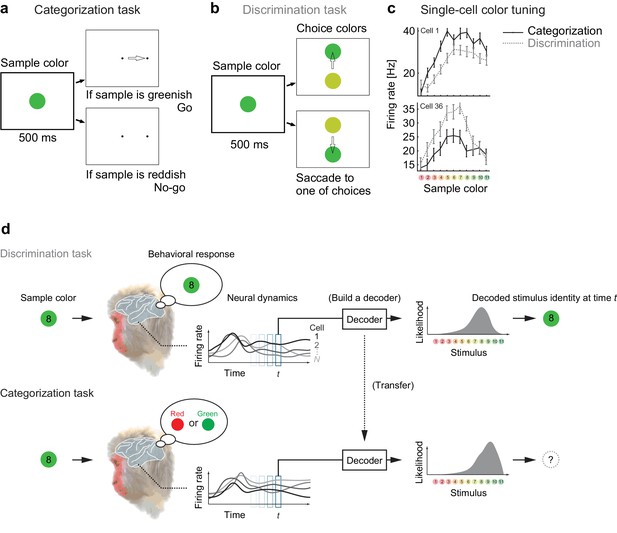
Color selectivity of IT neurons and the decoding-based stimulus reconstruction.
(a) In the categorization task, subjects classified sample colors into either a ‘reddish’ or ‘greenish’ group. (b) In the discrimination task, they selected the physically identical colors. (c) Color tuning curves of four representative neurons in the categorization and discrimination tasks. The color selectivity and task effect varied across neurons. The average firing rates during the period spanning 100–500 ms after stimulus onset are shown. The error bars indicate the s.e.m across trials. (d) The likelihood-based decoding for reconstructing the stimulus representation by the neural population.
-
Figure 1—source data 1
Neural tuning data.
Each neuron's response evoked by each color stimulus, where the firing rates were computed within each 50 ms time windows sliding with 10 ms time steps.
- https://doi.org/10.7554/eLife.26868.003
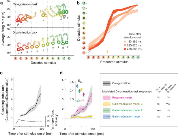
Population dynamics in the perceptual domain.
(a) State-space trajectories during the categorization and discrimination tasks. Small markers show the population states 100–550 ms after stimulus onset in 10 ms steps. Large markers indicate the endpoint (550 ms). The colors of the trajectories and numbers around them refer to the presented stimulus. (b) During the categorization task, the decoded stimulus was shifted toward either the ‘reddish’ or ‘greenish’ extreme during the late responses but not during the early responses. The thickness of the curve represents the 25th–75th percentile on resampling. The yellow arrow on the horizontal axis indicates the sample color corresponding to the categorical boundary estimated from the behavior (subject’s 50% response threshold) in the categorization task. (c) Evolution of the task-dependent clustering of the decoded stimulus (the curve with shade), as compared to the population average firing rate (the black solid and dashed curves). The magnitude of clustering was quantified with a clustering index, CI = (mean distance within categories) / (distance between category means) (Materials and methods). The figure shows the ratio of CIs in the two tasks, categorization/discrimination (smoothed with a 100 ms boxcar kernel for visualization). The horizontal line at CI ratio = 1 indicates the identity between the two tasks. The difference in CI ratio was larger in the late period (450–550 ms after the stimulus onset) than the early period (100–200 ms) (p=0.001, bootstrap test). The figure shows data averaged across all stimuli. The black curve and shaded area represent the median ±25 th percentile on the resampling. (d) The time-evolution of clustering indices in the gain-modulation and recurrent models applied to the discrimination-task data compared to the actual evolution in the categorization task (black curve, the same as in Figure 3c). The curve and shaded areas represent the median ±25 th percentile on the resampling. (Inset) The cross-validation errors () in model fitting measured based on the individual neurons’ firing rate (Materials and methods). The horizontal dashed line indicates the baseline variability in neural responses, which was quantified by comparing each neuron’s firing rate in the odd and even trials. In this plot, the results of the three gain modulation models are largely overlapped with each other. Error bars: the s.e.m. across neurons. G1: gain-modulation model 1; G2: gain-modulation model 2; G3: gain-modulation model 3; R: recurrent model.
-
Figure 2—source data 1
Neural tuning data.
Each neuron's response evoked by each color stimulus, where the firing rates were computed within each 50 ms time windows sliding with 10 ms time steps.
- https://doi.org/10.7554/eLife.26868.005
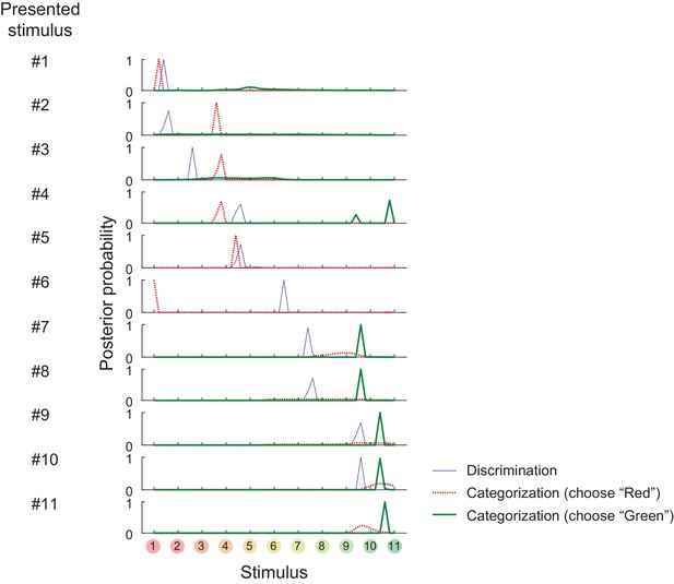
Posterior probability distributions in each stimulus and task.
https://doi.org/10.7554/eLife.26868.006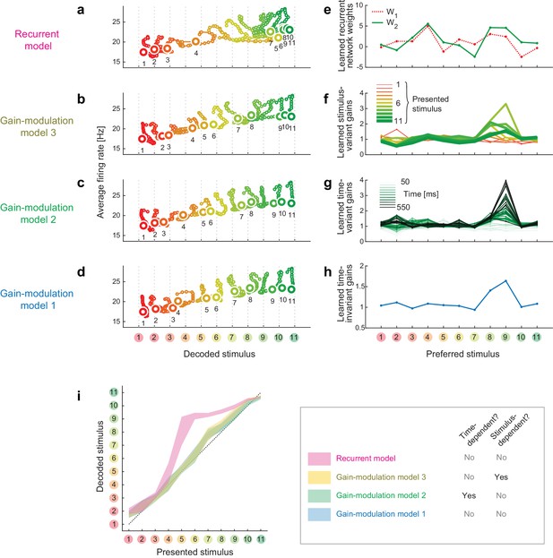
Trajectories and weights in trained models.
(a–d) Trajectories generated by the trained models. (e–h) The learned weights in the individual models. (i) The decoded vs. presented stimuli in the individual models.
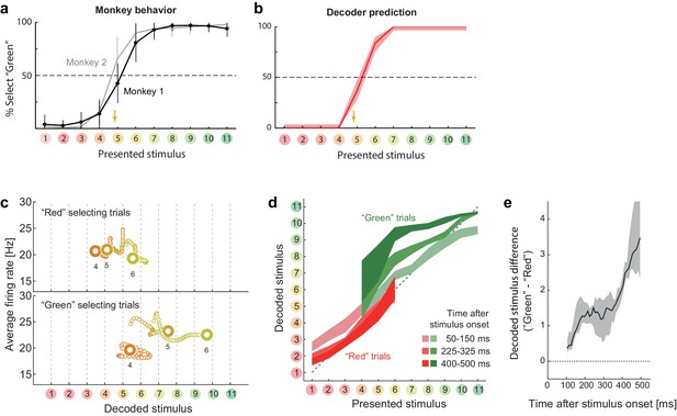
Choice-related dynamics.
(a) Actual monkey behavior. Note that the monkeys’ subjective category borders were consistent with the decoder output. The error bar is the standard error of mean. The yellow arrow on the horizontal axis indicates the sample color corresponding to the putative categorical boundary based on the behavior. (b) Fraction of selecting green category predicted by the likelihood-based decoding. The shaded area indicates the 25th–75th percentile on resampling. (c) The same analysis as Figure 2a (top) but with trial sets segregated based on whether the monkeys selected the ‘red’ or ‘green’ category. The results for stimuli #4–6 are shown. (d) The same analysis as Figure 2b, except that the trials were segregated based on the behavioral outcome. For stimuli #1–3 (#7–11), only the ‘Red’ (‘Green’) selecting trials were analyzed because the subjects rarely selected the other option for those stimuli. (e) Evolution of difference in the decoded color. Data were averaged across stimuli #4–6. The difference in the decoded stimulus was larger during the late period (450–550 ms) than the early period (50–150 ms) (p=0.002, permutation test).
-
Figure 3—source data 1
Neural tuning and population response data.
Each neuron's response evoked by each color stimulus, where the firing rates were computed within each 50 ms time windows sliding with 10 ms time steps, and the intermediate data summarizing the population responses.
- https://doi.org/10.7554/eLife.26868.009
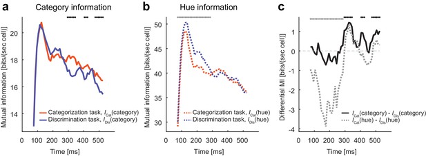
Modulation increases task-relevant information.
(a) The evolution of mutual information about category. (b) The evolution of mutual information about hue. (c) The evolution of the mutual information difference after the stimulus onset. The dots on top of each panel indicate the statistical significance (p<0.05, permutation test; black dots: larger category information in the categorization task; gray dots: larger hue information in the discrimination task; the dots on top of panel c just repeat the test results shown in panels a and b).
-
Figure 4—source data 1
Neural tuning and population response data.
Each neuron's response evoked by each color stimulus, where the firing rates were computed within each 50 ms time windows sliding with 10 ms time steps, and the intermediate data summarizing the population responses.
- https://doi.org/10.7554/eLife.26868.011
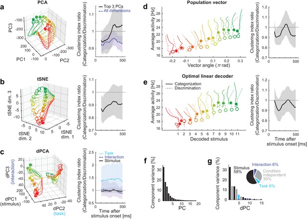
Comparison to other dimensionality reduction methods.
(a–e) The results of five different dimensionality reduction methods. (Left) the trajectories visualized in the reduced state space. (Right) The time evolutions of the clustering index ratio in each reduced space. The conventions follow that of Figure 2d. In (a–c), the trajectories in 0–550 ms after stimulus onset are shown; in (d, e), the trajectories in 100–550 ms after stimulus onset are shown, as in the Figure 2a, because the decoder outputs were unreliable before 100 ms. The filled and open circles indicate the end point (at 550 ms) of the trajectories in the categorization and discrimination tasks, respectively. The colors of trajectories indicate the presented stimuli (#1-11). The parameters used in each dimensionality reduction method is provided are provided in Materials and methods. (a) PCA. The left panel shows the top 3 principal components (PCs). The left panel depicts the clustering indices based on the top 3 components (black, solid) and all the neural activities (purple, dashed). (b) Three-dimensional space obtained by t-stochastic neighbor embedding (tSNE). (c) Demixed PCA (dPCA). The left panel shows the top component from each of stimulus-dependent (black, solid), task-dependent (cyan, dotted), and stimulus-task-interaction (purple, dashed) components. (d) Population vector decoding. The horizontal and vertical axes show the decoder output and the average firing rate in population, respectively. (e) Optimal linear decoder. The horizontal and vertical axes show the decoder output and the average firing rate in population, respectively. (f) The fraction of data variance explained by each principal component (PC) in PCA. (g) The fraction of data variance explained by each demixed component (dPC) in dPCA. (Inset) The pie chart showing the relative contributions of stimulus, task, interaction and condition-independent components.
-
Figure 5—source data 1
Neural tuning and population response data.
Each neuron's response evoked by each color stimulus, where the firing rates were computed within each 50 ms time windows sliding with 10 ms time steps, and the intermediate data summarizing the population responses.
- https://doi.org/10.7554/eLife.26868.013
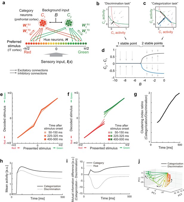
Bifurcation of attractor dynamics in a simple neural circuit model.
(a) Schematic of the model circuit architecture. IT hue-selective neurons (hereafter, hue-neurons), , with different preferred stimuli (varying from red to green) receive sensory input, , from the earlier visual cortex. The hue neurons interact with category neuron groups and through bottom-up and top-down connections with weights (, ) and (, ), respectively. The category neurons also receive a common background input, , whose magnitude depends on task context. Note that the modeled hue-neurons covered entire hue circle, [-π, π], although the figure shows only the half of them, corresponding to the stimulus range from red to green. (b) Activity evolution represented in the space of category-neurons in the discrimination task (where the background input ). The red (dashed) and green (solid) curves represent nullclines for category-neurons 1 and 2, respectively. The black line shows a dynamical trajectory, starting from (0, 0) and ending at a filled circle. The gray arrows schematically illustrate the vector field. (c) The same analysis as in panel c but in the categorization task (where ). The black and blue lines show two different dynamical trajectories, starting from (−0.01, 0.01) and (−0.01, 0.01), respectively (indicated as numbers ‘1’ and ‘2’ in the figure), and separately ending at filled circles. (d) The number of stable fixed points is controlled by the parameter B. Here, the parameter B was continuously varied as the bifurcation parameter while the other parameters were kept constant. The vertical axis shows the difference of category neuron activities, , corresponding to the fixed points. The solid black and blue curves show the stable fixed points; the dashed line indicates the unstable fixed point. The stimulus value was s = 0. (e–k) The model replicates recorded neural population dynamics. (e) Presented and decoded stimuli. The same analysis as in Figure 2b was applied to the dynamics of the modeled hue-neurons. (f) The same as panel e, except that the trials were segregated based on the choices (i.e., to which fixed point the neural states were attracted). The plot corresponds to Figure 3d. (g) Evolution of difference in the decoded color, corresponding to Figure 3e. (h) Mean activity of the entire neural population, corresponding to Figure 2c, inset. (i) Differences in mutual information about category and hue between the categorization and discrimination tasks, corresponding to Figure 4c. (j) The activity trajectories of the modeled hue-neurons population in PCA space, corresponding to Figure 5a. Note that the scaling of the stimulus coordinate (ranging from to ) used in the model is not necessarily identical to that of experimental stimuli (index by colors #1 – #11), and point of this modeling is to replicate the qualitative aspects of the data.

Nullclines in different stimulus conditions and background input.
Under a strong background inhibition (, corresponding to the ‘discrimination task’), the system always have only one stable fixed point. On the other hand, under a weak background inhibition, (, corresponding to the ‘categorization task’), the system can have two stable fixed points for the neutral stimuli (). This is consistent with the monkey behavior that was more variable for the neutral stimuli compared to the stimuli at the reddish/greenish category extreme. The convention follows that of Figure 6b and c.
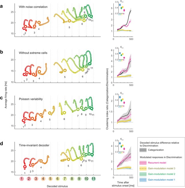
Robustness of the results to changes in the decoder.
We replicated the main results of the paper using four different decoders. Both the stimulus-dependent clustering effect and the temporal evolution were replicated with those decoders. (Left) State-space trajectories during the categorization task (corresponding to Figure 2a, top). (Right) Time-evolution of clustering indices in the gain modulation and recurrent models compared to that in the categorization-task data (corresponding to Figure 2d). (a) Results obtained by simulating noise correlation among neurons. Here we assumed that the covariance between two different neurons, i and j, is proportional to the correlation between their mean spike counts (Cohen and Kohn, 2011; Pitkow et al., 2015): , where k is a constant shared across all neuron pairs (here, ), and is the Fano factor for neuron . (b) Results based on a subset of the recorded cell population; excluded are cells showing extremely high or low activity, as compared to the typical firing rate of the population. We only used cells whose average firing rates (the average across all stimuli and time bins) were within the 25th-75th percentile of the whole population. (c) Results with a decoder based on Poisson spike variability. The generative model of neuron i’s spike count in response to stimulus s at time t was given by (i.e., the log likelihood was provided by ). (d) Results with a time-invariant decoder. The mean and variance of each neuron’s spike count were computed by pooling all the time bins during the period spanning 200–550 ms after stimulus onset.
-
Figure 7—source data 1
Neural tuning and population response data.
Each neuron's response evoked by each color stimulus, where the firing rates were computed within each 50 ms time windows sliding with 10 ms time steps, and the intermediate data summarizing the population decoding results.
- https://doi.org/10.7554/eLife.26868.017
Additional files
-
Source code file 1
Related to Figure 1: Matlab codes related to Figure 1.
The codes run with Figure 1—source data 1.
- https://doi.org/10.7554/eLife.26868.018
-
Source code file 2
Related to Figure 2: Matlab codes related to Figure 2.
The codes run with Figure 2—source data 1.
- https://doi.org/10.7554/eLife.26868.019
-
Source code file 3
Related to Figure 3: Matlab codes related to Figure 3.
The codes run with Figure 3—source data 1.
- https://doi.org/10.7554/eLife.26868.020
-
Source code file 4
Related to Figure 4: Matlab codes related to Figure 4.
The codes run with Figure 4—source data 1.
- https://doi.org/10.7554/eLife.26868.021
-
Source code file 5
Related to Figure 5: Matlab codes related to Figure 5.
The codes run with Figure 5—source data 1.
- https://doi.org/10.7554/eLife.26868.022
-
Source code file 6
Related to Figure 6: Matlab codes related to Figure 6.
The codes simulate the neural population response based on the recurrent differential equation model described in the text.
- https://doi.org/10.7554/eLife.26868.023
-
Source code file 7
Related to Figure 7: Matlab codes related to Figure 7.
The codes run with Figure 7—source data 1.
- https://doi.org/10.7554/eLife.26868.024


