Efficient and accurate extraction of in vivo calcium signals from microendoscopic video data
- Carnegie Mellon University, United States
- Columbia University, United States
- University of North Carolina at Chapel Hill, United States
- New York State Psychiatric Institute, United States
- Harvard Medical School, Howard Hughes Medical Institute, United States
- Flatiron Institute, Simons Foundation, United States
- University of California, San Francisco, United States
- University of California, United States
Figures
Figure 1
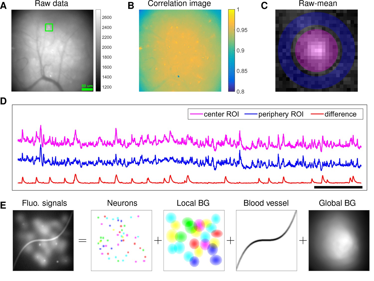
Microendoscopic data contain large background signals with rapid fluctuations due to multiple sources.
(A) An example frame of microendoscopic data recorded in dorsal striatum (see Materials and methods section for experimental details). (B) The local ‘correlation image’ (Smith and Häusser, 2010) computed from the raw video data. Note that it is difficult to discern neuronal shapes in this image due to the high background spatial correlation level. (C) The mean-subtracted data within the cropped area (green) in (A). Two ROIs were selected and coded with different colors. (D) The mean fluorescence traces of pixels within the two selected ROIs (magenta and blue) shown in (C) and the difference between the two traces. (E) Cartoon illustration of various sources of fluorescence signals in microendoscopic data. ‘BG’ abbreviates ‘background’.
Figure 2
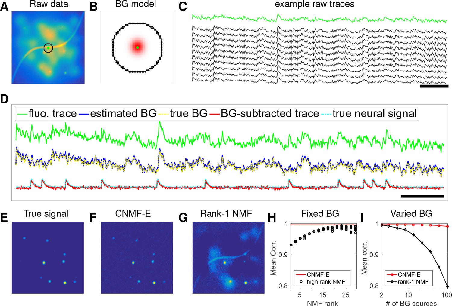
CNMF-E can accurately separate and recover the background fluctuations in simulated data.
(A) An example frame of simulated microendoscopic data formed by summing up the fluorescent signals from the multiple sources illustrated in Figure 1E. (B) A zoomed-in version of the circle in (A). The green dot indicates the pixel of interest. The surrounding black pixels are its neighbors with a distance of 15 pixels. The red area approximates the size of a typical neuron in the simulation. (C) Raw fluorescence traces of the selected pixel and some of its neighbors on the black ring. Note the high correlation. (D) Fluorescence traces (raw data; true and estimated background; true and initial estimate of neural signal) from the center pixel as selected in (B). Note that the background dominates the raw data in this pixel, but nonetheless we can accurately estimate the background and subtract it away here. Scalebars: seconds. Panels (E–G) show the cellular signals in the same frame as (A). (E) Ground truth neural activity. (F) The residual of the raw frame after subtracting the background estimated with CNMF-E; note the close correspondence with E. (G) Same as (F), but the background is estimated with rank-1 NMF. A video showing (E–G) for all frames can be found at Video 2. (H) The mean correlation coefficient (over all pixels) between the true background fluctuations and the estimated background fluctuations. The rank of NMF varies and we run randomly-initialized NMF for 10 times for each rank. The red line is the performance of CNMF-E, which requires no selection of the NMF rank. (I) The performance of CNMF-E and rank-1 NMF in recovering the background fluctuations from the data superimposed with an increasing number of background sources.
Figure 3
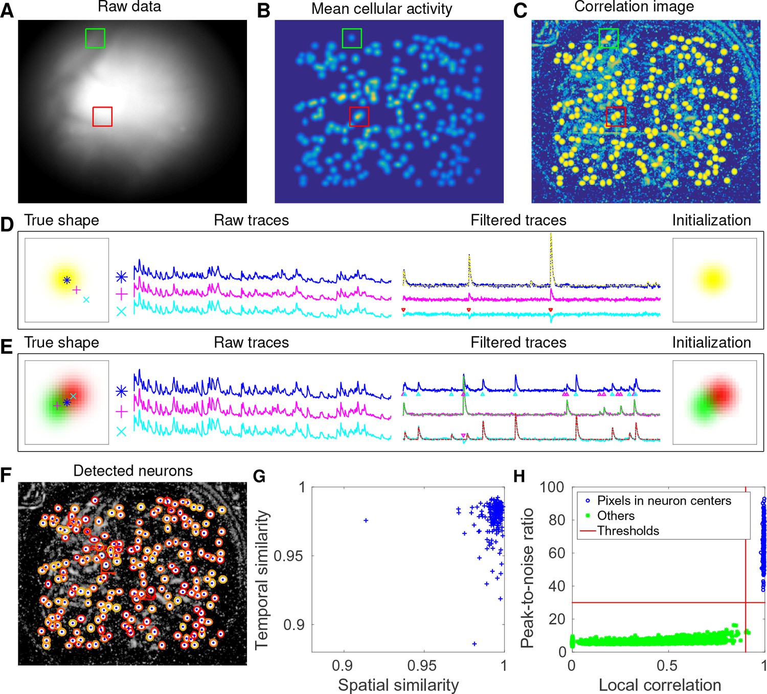
CNMF-E accurately initializes individual neurons’ spatial and temporal components in simulated data.
(A) An example frame of the simulated data. Green and red squares will correspond to panels (D) and (E) below, respectively. (B) The temporal mean of the cellular activity in the simulation. (C) The correlation image computed using the spatially filtered data. (D) An example of initializing an isolated neuron. Three selected pixels correspond to the center, the periphery, and the outside of a neuron. The raw traces and the filtered traces are shown as well. The yellow dashed line is the true neural signal of the selected neuron. Triangle markers highlight the spike times from the neuron. (E) Same as (D), but two neurons are spatially overlapping in this example. Note that in both cases neural activity is clearly visible in the filtered traces, and the initial estimates of the spatial footprints are already quite accurate (dashed lines are ground truth). (F) The contours of all initialized neurons on top of the correlation image as shown in (D). Contour colors represent the rank of neurons’ SNR (SNR decreases from red to yellow). The blue dots are centers of the true neurons. (G) The spatial and the temporal cosine similarities between each simulated neuron and its counterpart in the initialized neurons. (H) The local correlation and the peak-to-noise ratio for pixels located in the central area of each neuron (blue) and other areas (green). The red lines are the thresholding boundaries for screening seed pixels in our initialization step. A video showing the whole initialization step can be found at Video 3.
Figure 4
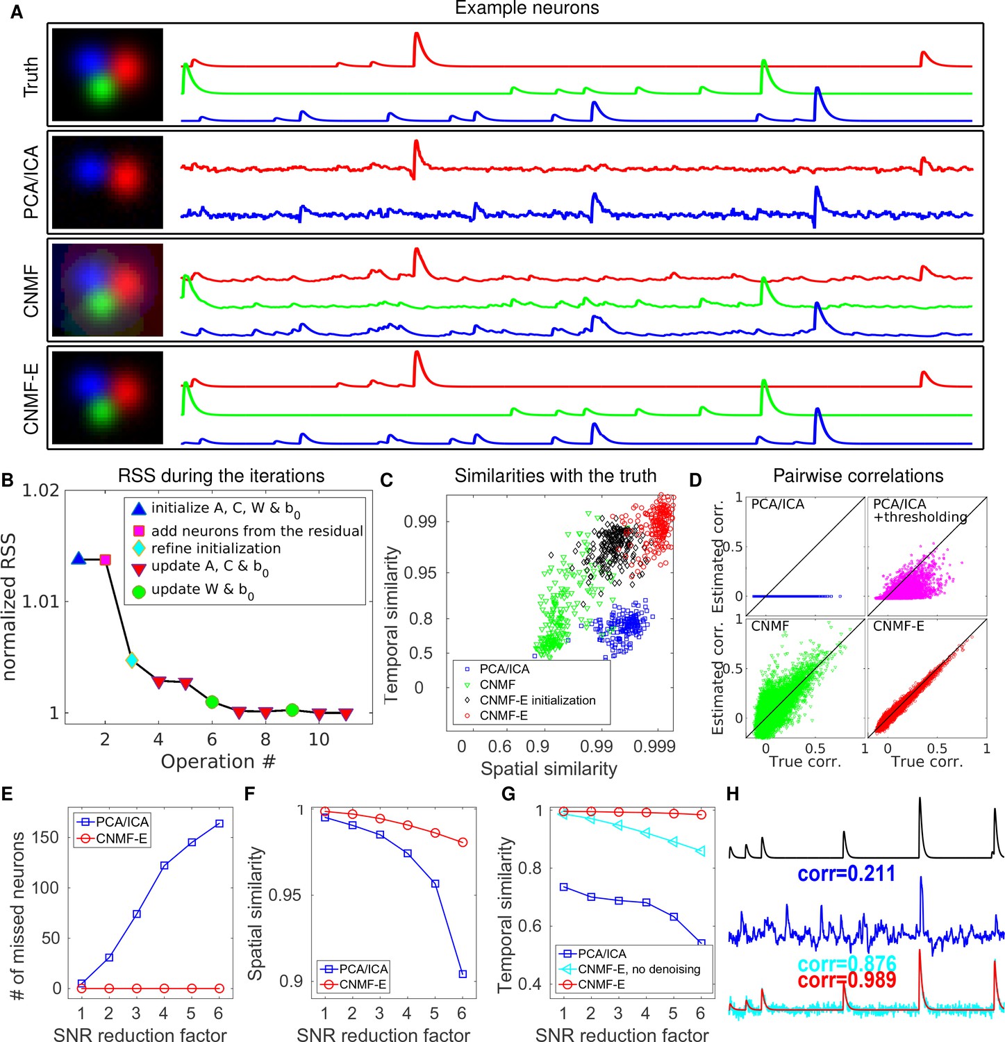
CNMF-E outperforms PCA/ICA analysis in extracting individual neurons’ activity from simulated data and is robust to low SNR.
(A) The results of PCA/ICA, CNMF, and CNMF-E in recovering the spatial footprints and temporal traces of three example neurons. The trace colors match the neuron colors shown in the left. (B) The intermediate residual sum of squares (RSS) values (normalized by the final RSS value), during the CNMF-E model fitting. The 'refine initialization’ step refers to the modification of the initialization results in the case of high temporal correlation (details in Materials and methods). (C) The spatial and the temporal cosine similarities between the ground truth and the neurons detected using different methods. (D) The pairwise correlations between the calcium activity traces extracted using different methods. (E–G) The performances of PCA/ICA and CNMF-E under different noise levels: the number of missed neurons (E), and the spatial (F) and temporal (G) cosine similarities between the extracted components and the ground truth. (H) The calcium traces of one example neuron: the ground truth (black), the PCA/ICA trace (blue), the CNMF-E trace (red) and the CNMF-E trace without being denoised (cyan). The similarity values shown in the figure are computed as the cosine similarity between each trace and the ground truth (black). Two videos showing the demixing results of the simulated data can be found in Video 4 (SNR reduction factor = 1) and Video 5 (SNR reduction factor = 6).
Figure 5
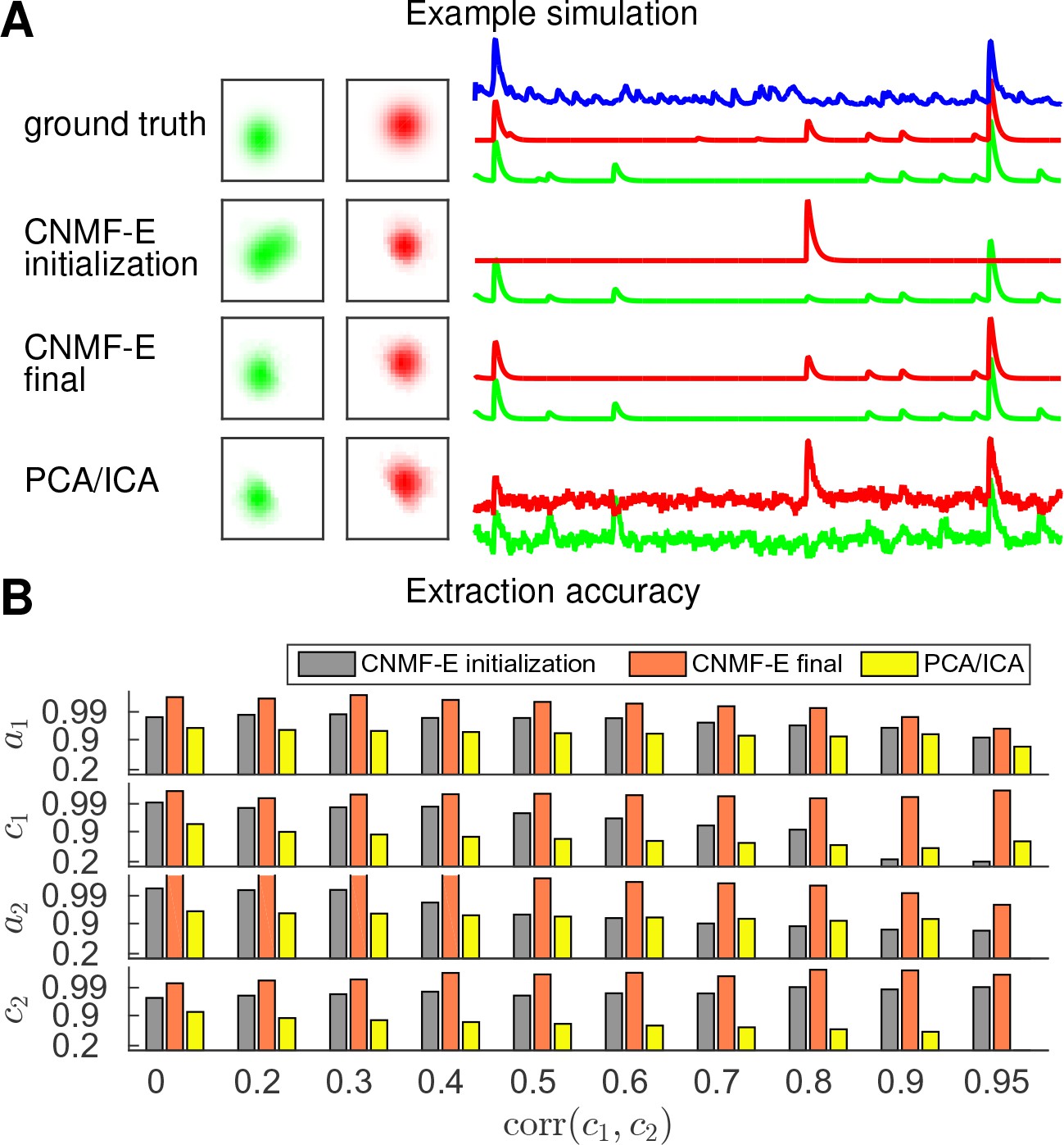
CNMF-E is able to demix neurons with high temporal correlations.
(A) An example simulation from the experiments summarized in panel (B), where is 0.9: green and red traces correspond to the corresponding neuronal shapes in the left panels. The blue trace is the mean background fluorescence fluctuation over the whole FOV. (B) The extraction accuracy of the spatial ( and ) and the temporal ( and ) components of two close-by neurons, computed via the cosine similarity between the ground truth and the extraction results.
Figure 6
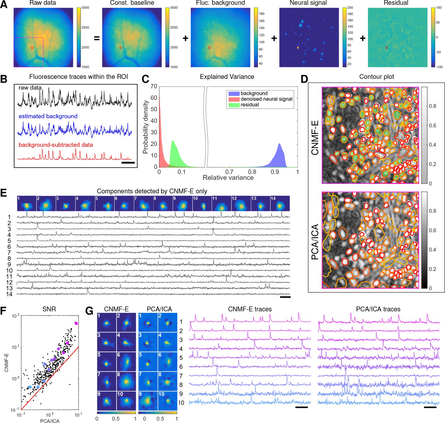
Neurons expressing GCaMP6f recorded in vivo in mouse dorsal striatum area.
(A) An example frame of the raw data and its four components decomposed by CNMF-E. (B) The mean fluorescence traces of the raw data (black), the estimated background activity (blue), and the background-subtracted data (red) within the segmented area (red) in (A). The variance of the black trace is about 2x the variance of the blue trace and 4x the variance of the red trace. (C) The distributions of the variance explained by different components over all pixels; note that estimated background signals dominate the total variance of the signal. (D) The contour plot of all neurons detected by CNMF-E and PCA/ICA superimposed on the correlation image. Green areas represent the components that are only detected by CNMF-E. The components are sorted in decreasing order based on their SNRs (from red to yellow). (E) The spatial and temporal components of 14 example neurons that are only detected by CNMF-E. These neurons all correspond to green areas in (D). (F) The signal-to-noise ratios (SNRs) of all neurons detected by both methods. Colors match the example traces shown in (G), which shows the spatial and temporal components of 10 example neurons detected by both methods. Scalebar: 10 s. See Video 6 for the demixing results.
Figure 7
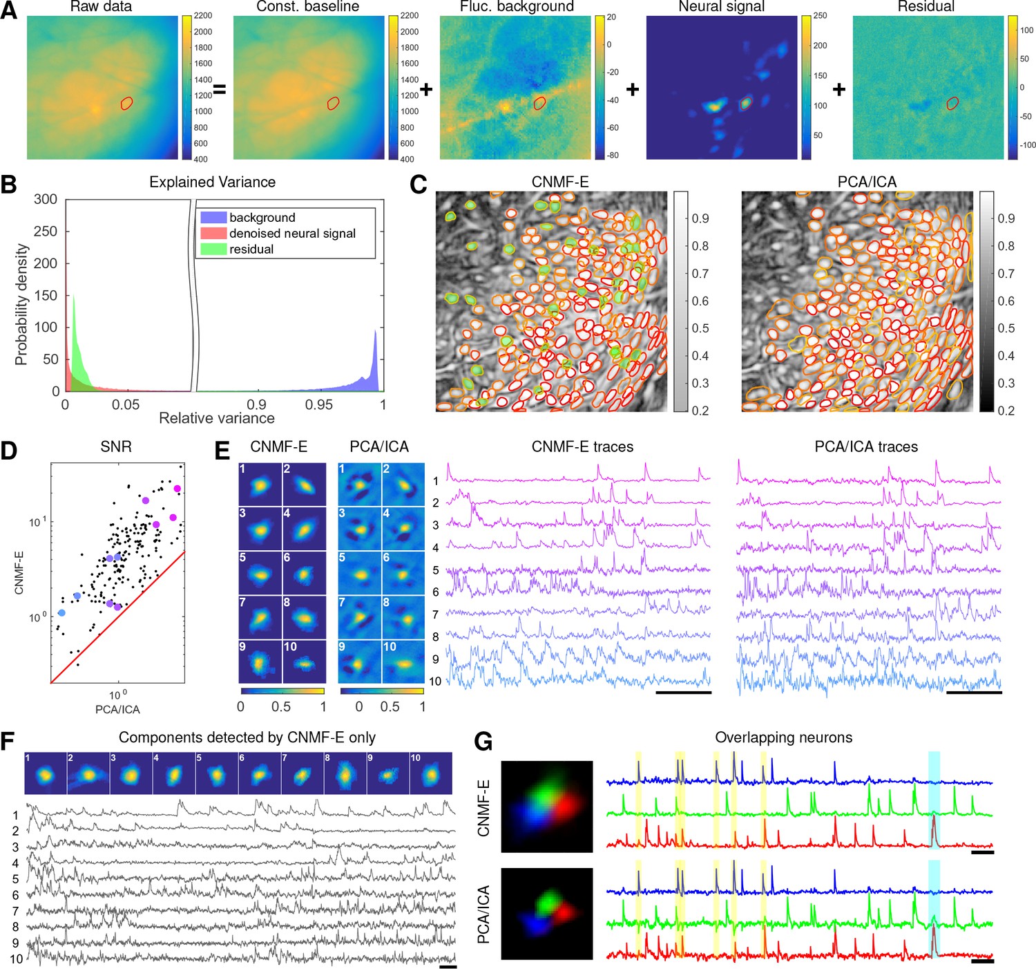
Neurons expressing GCaMP6s recorded in vivo in mouse prefrontal cortex.
(A–F) follow similar conventions as in the corresponding panels of Figure 6. (G) Three example neurons that are close to each other and detected by both methods. Yellow shaded areas highlight the negative ‘spikes’ correlated with nearby activity, and the cyan shaded area highlights one crosstalk between nearby neurons. Scalebar: 20 s. See Video 7 for the demixing results and Video 8 for the comparision of CNMF-E and PCA/ICA in the zoomed-in area of (G).
Figure 8
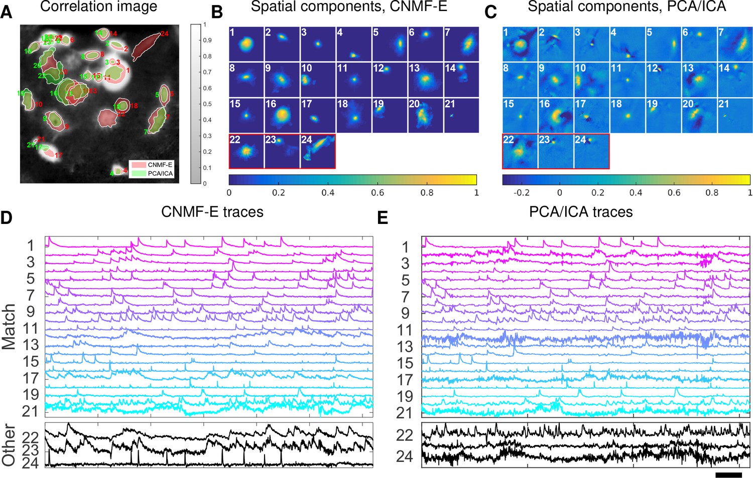
Neurons expressing GCaMP6f recorded in vivo in mouse ventral hippocampus.
(A) Contours of all neurons detected by CNMF-E (red) and PCA/ICA method (green). The grayscale image is the local correlation image of the background-subtracted video data, with background estimated using CNMF-E. (B) Spatial components of all neurons detected by CNMF-E. The neurons in the first three rows are also detected by PCA/ICA, while the neurons in the last row are only detected by CNMF-E. (C) Spatial components of all neurons detected by PCA/ICA; similar to (B), the neurons in the first three rows are also detected by CNMF-E and the neurons in the last row are only detected by PCA/ICA method. (D) Temporal traces of all detected components in (B). ‘Match’ indicates neurons in top three rows in panel (B); ‘Other’ indicates neurons in the fourth row. (E) Temporal traces of all components in (C). Scalebars: seconds. See Video 9 for demixing results.
Figure 9
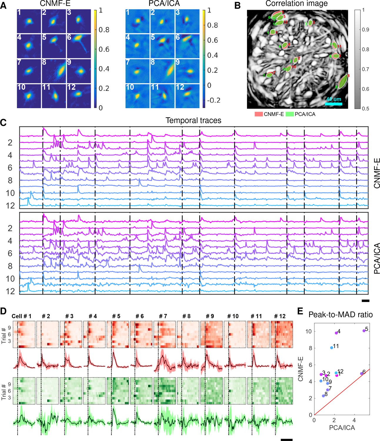
Neurons extracted by CNMF-E show more reproducible responses to footshock stimuli, with larger signal sizes relative to the across-trial variability, compared to PCA/ICA.
(A–C) Spatial components (A), spatial locations (B) and temporal components (C) of 12 example neurons detected by both CNMF-E and PCA/ICA. (D) Calcium responses of all example neurons to footshock stimuli. Colormaps show trial-by-trial responses of each neuron, extracted by CNMF-E (top, red) and PCA/ICA (bottom, green), aligned to the footshock time. The solid lines are medians of neural responses over 11 trials and the shaded areas correpond to median median absolute deviation (MAD). Dashed lines indicate the shock timings. (E) Scatter plot of peak-to-MAD ratios for all response curves in (D). For each neuron, Peak is corrected by subtracting the mean activity within 4 s prior to stimulus onset and MAD is computed as the mean MAD values over all timebins shown in (D). The red line shows . Scalebars: 10 s. See Video 11 for demixing results.
Figure 10
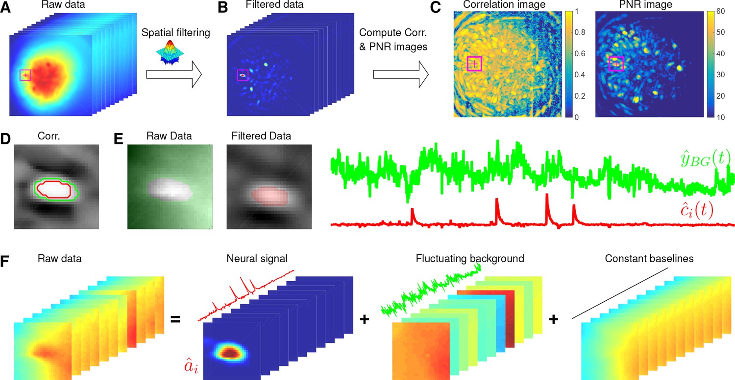
Illustration of the initialization procedure.
(A) Raw video data and the kernel for filtering the video data. (B) The spatially high-pass filtered data. (C) The local correlation image and the peak-to-noise ratio (PNR) image calculated from the filtered data in (B). (D) The temporal correlation coefficients between the filtered traces (B) of the selected seed pixel (the red cross) and all other pixels in the cropped area as shown in (A–C). The red and green contour correspond to correlation coefficients equal to 0.7 and 0.3, respectively. (E) The estimated background fluctuation (green) and the initialized temporal trace of the neuron (red). is computed as the median of the raw fluorescence traces of all pixels (green area) outside of the green contour shown in (D) and is computed as the mean of the filtered fluorescence traces of all pixels inside the red contour. (F) The decomposition of the raw video data within the cropped area. Each component is a rank- matrix and the related temporal traces are estimated in (E). The spatial components are estimated by regressing the raw video data against these three traces. See Video 3 for an illustration of the initialization procedure.
Videos
Video 1
An example of typical microendoscopic data.
The video was recorded in dorsal striatum; experimental details can be found above. MP4
Video 2
Comparison of CNMF-E with rank-1 NMF in estimating background fluctuation in simulated data.
Top left: the simulated fluorescence data in Figure 2. Bottom left: the ground truth of neuron signals in the simulation. Top middle: the estimated background from the raw video data (top left) using CNMF-E. Bottom middle: the residual of the raw video after subtracting the background estimated with CNMF-E. Top right and top bottom: same as top middle and bottom middle, but the background is estimated with rank-1 NMF. MP4
Video 3
Initialization procedure for the simulated data in Figure 3.
Top left: correlation image of the filtered data. Red dots are centers of initialized neurons. Top middle: candidate seed pixels (small red dots) for initializing neurons on top of PNR image. The large red dot indicates the current seed pixel. Top right: the correlation image surrounding the selected seed pixel or the spatial footprint of the initialized neuron. Bottom: the filtered fluorescence trace at the seed pixel or the initialized temporal activity (both raw and denoised). MP4
Video 4
The results of CNMF-E in demixing simulated data in Figure 4 (SNR reduction factor = 1).
Top left: the simulated fluorescence data. Bottom left: the estimated background. Top middle: the residual of the raw video (top left) after subtracting the estimated background (bottom left). Bottom middle: the denoised neural signals. Top right: the residual of the raw video data (top right) after subtracting the estimated background (bottom left) and denoised neural signal (bottom middle). Bottom right: the ground truth of neural signals in simulation. MP4
Video 5
The results of CNMF-E in demixing the simulated data in Figure 4 (SNR reduction factor = 6).
Conventions as in previous video. MP4
Video 6
The results of CNMF-E in demixing dorsal striatum data.
Top left: the recorded fluorescence data. Bottom left: the estimated background. Top middle: the residual of the raw video (top left) after subtracting the estimated background (bottom left). Bottom middle: the denoised neural signals. Top right: the residual of the raw video data (top right) after subtracting the estimated background (bottom left) and denoised neural signal (bottom middle). Bottom right: the denoised neural signals while all neurons’ activity are coded with pseudocolors. MP4
Video 7
The results of CNMF-E in demixing PFC data.
Conventions as in previous video. MP4
Video 8
Comparison of CNMF-E with PCA/ICA in demixing overlapped neurons in Figure 7G.
Top left: the recorded fluorescence data. Bottom left: the residual of the raw video (top left) after subtracting the estimated background using CNMF-E. Top middle and top right: the spatiotemporal activity and temporal traces of three neurons extracted using CNMF-E. Bottom middle and bottom right: the spatiotemporal activity and temporal traces of three neurons extracted using PCA/ICA. MP4
Video 9
The results of CNMF-E in demixing ventral hippocampus data.
Conventions as in Video 6. MP4
Video 10
Extracted spatial and temporal components of CNMF-E at different stages (ventral hippocampal dataset).
After initializing components, we ran matrix updates and interventions in automatic mode, resulting in components in total. In the next iteration, we manually deleted components and automatically merged neurons as well. In the last iterations, neurons were merged into neurons with manual verifications. The correlation image in the top left panel is computed from the background-subtracted data in the final step. MP4
Video 11
The results of CNMF-E in demixing BNST data.
Conventions as in Video 6. MP4
Tables
Table 1
Variables used in the CNMF-E model and algorithm. : real numbers; : positive real numbers; : natural numbers; : positive integers.
https://doi.org/10.7554/eLife.28728.006| Name | Description | Domain |
|---|---|---|
| number of pixels | ||
| number of frames | ||
| number of neurons | ||
| motion corrected video data | ||
| spatial footprints of all neurons | ||
| temporal activities of all neurons | ||
| background activity | ||
| observation noise | ||
| weight matrix to reconstruct using neighboring pixels | ||
| constant baseline for all pixels | ||
| spatial location of the th pixel | ||
| standard deviation of the noise at pixel |
Table 2
Optional user-specified parameters.
https://doi.org/10.7554/eLife.28728.024| Name | Description | Default values | Used in |
|---|---|---|---|
| size of a typical neuron soma in the FOV | Algorithm 1 | ||
| the distance between each pixel and its neighbors | Problem (P-B) | ||
| the minimum peak-to-noise ratio of seed pixels | 10 | Algorithm 1 | |
| the minimum local correlation of seed pixels | 0.8 | Algorithm 1 | |
| the ratio between the outlier threshold and the noise | 10 | Problem (P-B) |
Table 3
Running time (sec) for processing the 4 experimental datasets.
https://doi.org/10.7554/eLife.28728.025| Dataset | Striatum | PFC | Hippocampus | BNST |
|---|---|---|---|---|
| Size (x × y × t) | 256 × 256 × 6000 | 175 × 184 × 9000 | 175 × 184 × 9000 | 175 × 184 × 9000 |
| (# PCs, # ICs) | (2000, 700) | (275, 250) | (100, 50) | (200, 150) |
| PFC/ICA | 986 | 181 | 174 | 52 |
| CNMF-E | 726 | 221 | 225 | 435 |
Additional files
-
Transparent reporting form
- https://doi.org/10.7554/eLife.28728.026
Download links
A two-part list of links to download the article, or parts of the article, in various formats.
Downloads (link to download the article as PDF)
Open citations (links to open the citations from this article in various online reference manager services)
Cite this article (links to download the citations from this article in formats compatible with various reference manager tools)
Efficient and accurate extraction of in vivo calcium signals from microendoscopic video data
eLife 7:e28728.
https://doi.org/10.7554/eLife.28728


