Computer assisted detection of axonal bouton structural plasticity in in vivo time-lapse images
- Northeastern University, United States
- University of Geneva, Switzerland
- Lemanic Neuroscience Doctoral School, Switzerland
- École Polytechnique Fédérale de Lausanne, Switzerland
Figures
Figure 1
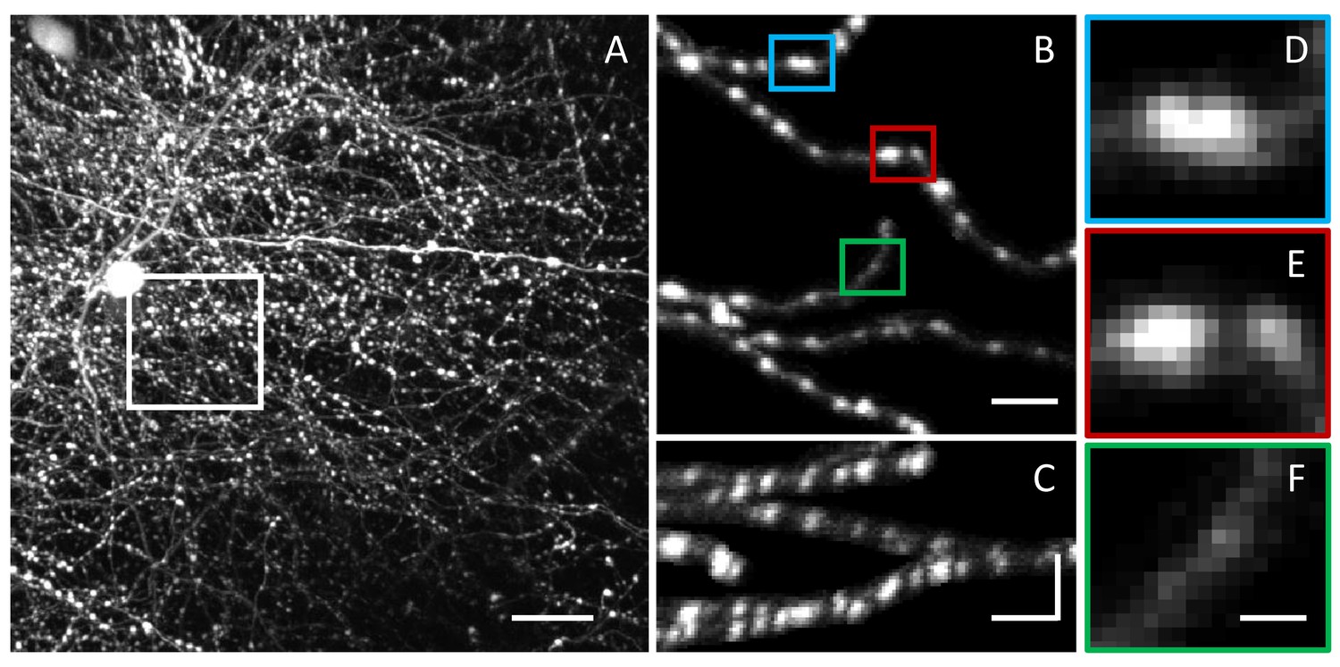
Challenges in LM-based bouton detection and measurement.
(A) Maximum intensity xy projection of an image stack showing axons of fluorescently labeled neurons in superficial layers of mouse barrel cortex. High density of labeled axons makes it difficult to automatically detect boutons and track their structural changes over time. Scale bar is 20 μm. (B) A subset of labeled axons from the region outlined in (A). To improve visibility, image intensity beyond five voxels from the axon centerlines was set to zero. Bouton detection and bouton size measurement are confounded by large variations in fluorescence levels across axons. (C) Axons from (B) shown on the zx maximum intensity projection. Horizontal scale bars in (B) and (C) are 5 μm. Vertical scale bar in (C) is 15 μm. Lower resolution in z compared to xy is yet another challenge in bouton analyses. (D–F) Magnified views of the highlighted boutons from (B). Close proximity of boutons on an axon (D), large range of bouton sizes (E), and large range of bouton fluorescence levels (D–F), present additional obstacles to accurate bouton detection and measurement. Scale bar in (D–F) is 1.25 μm.
Figure 2 with 2 supplements
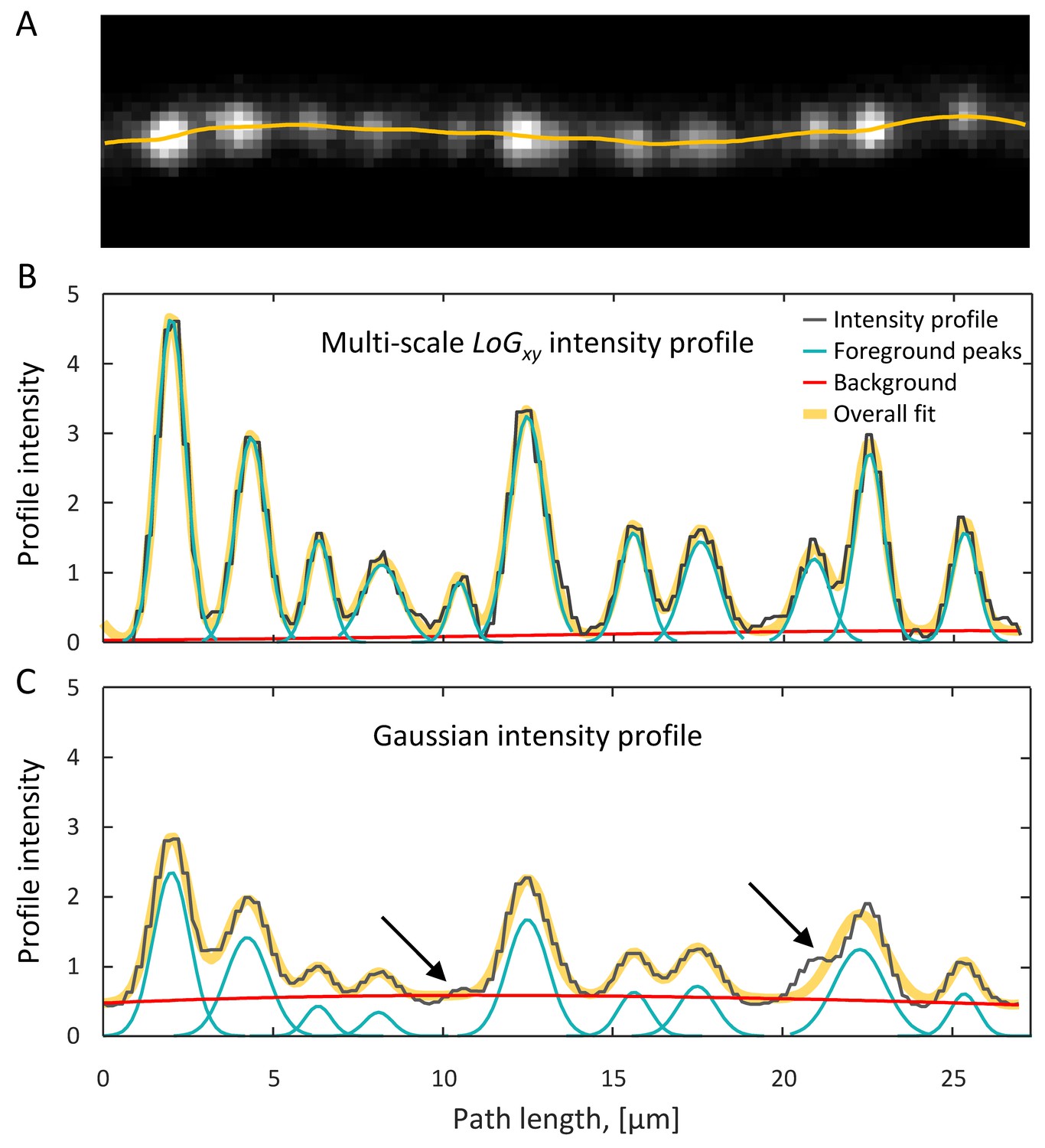
Detection of putative boutons as peaks on axon intensity profiles.
(A) Maximum intensity xy projection of an axon segment showing multiple putative boutons. Yellow line is the optimized trace of this axon. (B) Putative boutons visible in (A) correspond to peaks on the LoGxy intensity profile (black line). Foreground peaks (cyan lines) and local background (red line) are fitted to the intensity profile as described in the text. The overall fit (thick yellow line), which is the sum of foreground peaks and background, closely matches the intensity profile. (C) G intensity profile is obtained by sliding a fixed size Gaussian filter along the optimized trace. Small or closely positioned peaks cannot be resolved on the G profile (arrows). Peak amplitudes from the LoGxy profile and background from the G profile are used to define bouton weights.
Figure 2—figure supplement 1
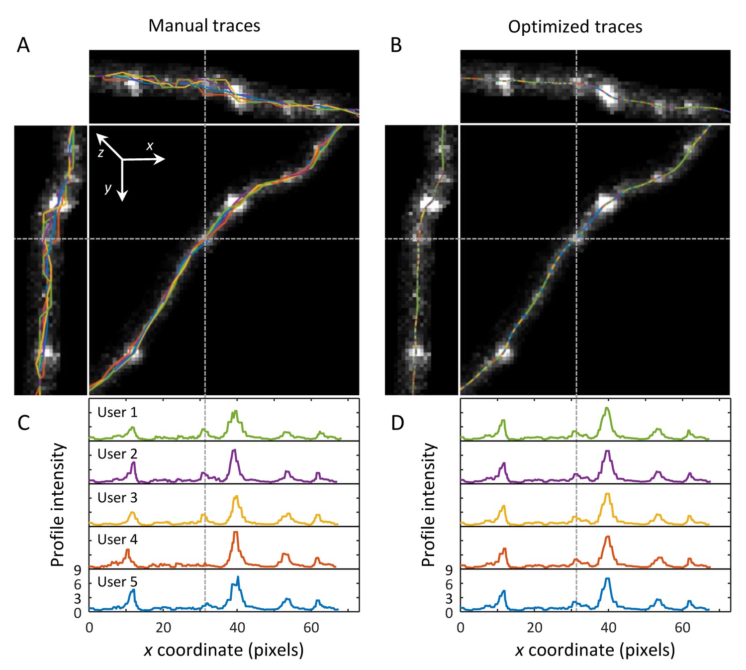
Optimization is required for trace-based bouton detection and measurement.
(A) Five users traced the same set of 16 axon segments using manual tracing module of NCTracer software. Manual traces (colored lines) are shown superimposed on zx (top), yz (left), and xy (center) maximum intensity projection images of an axon segment. To improve visibility, image intensity beyond five voxels from the axon centerline was set to zero. While on the xy projection, manual traces closely match the underlying axon intensity, variability between traces becomes apparent by viewing the zx and yz projections. (B) User traces after optimization are virtually indistinguishable on all projections. (C) Axon intensity profiles can be obtained by sliding various filters along manual traces. Here, we show LoGxy intensity profiles for the five manual user traces. Note that slight tracing inaccuracies may lead to large variability in axon intensity profiles, e.g. absent peak in the User four trace profile (dashed line). (D) Inter-user variability in axon intensity profiles is virtually eliminated after trace optimization.
Figure 2—figure supplement 2
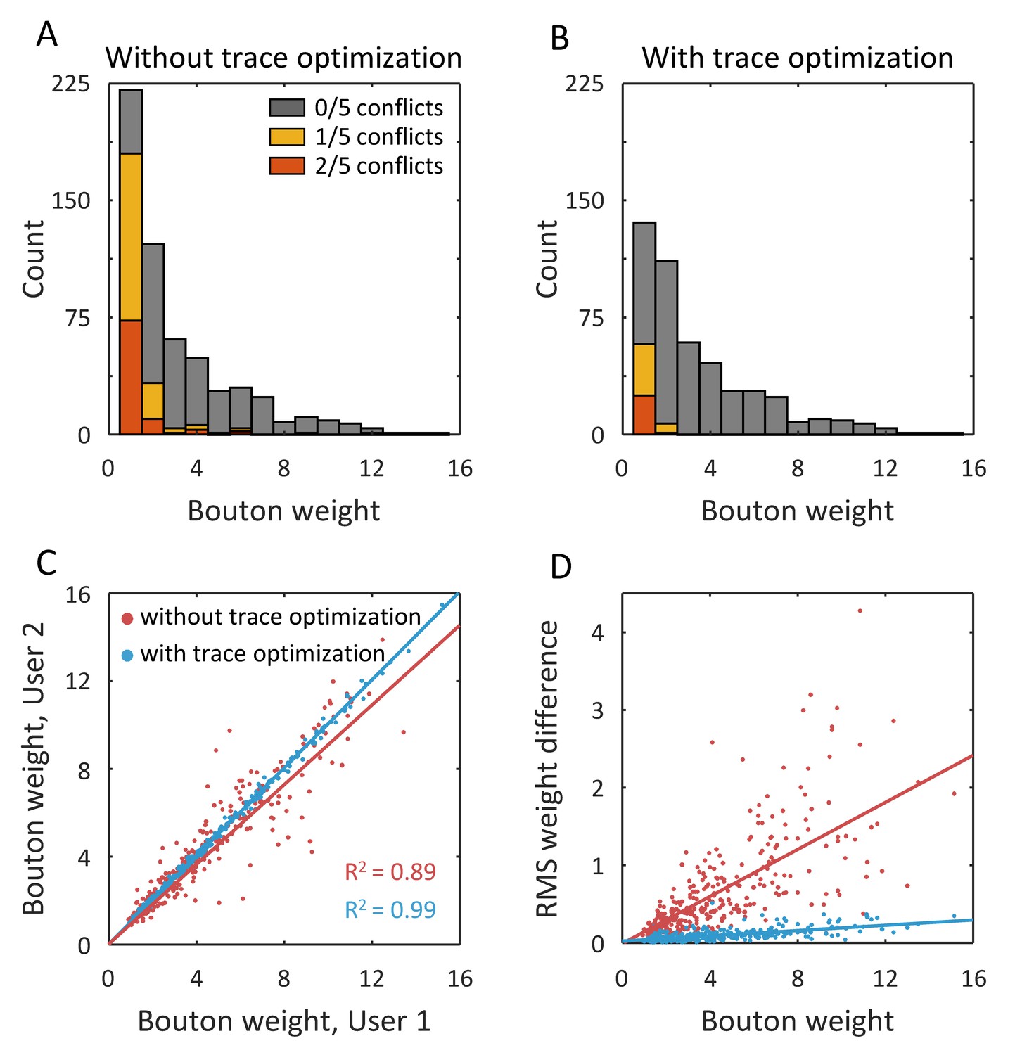
Trace optimization reduces variability in bouton detection and weight measurement.
(A) Putative boutons were automatically detected based on manual traces of 5 users. Differences in user traces lead to variability in putative bouton detection. The fraction of inter-user conflicts is particularly high for low weight boutons. (B) Trace optimization reduces the fraction of inter-user conflicts. (C) Trace optimization also reduces inter-user bias and variability in bouton weight measurements. (D) Root mean square (RMS) weight difference, calculated for putative boutons detected on manual (red points) and optimized traces (blue points), shows that optimization reduces variability in the entire range of bouton weights.
Figure 3 with 1 supplement
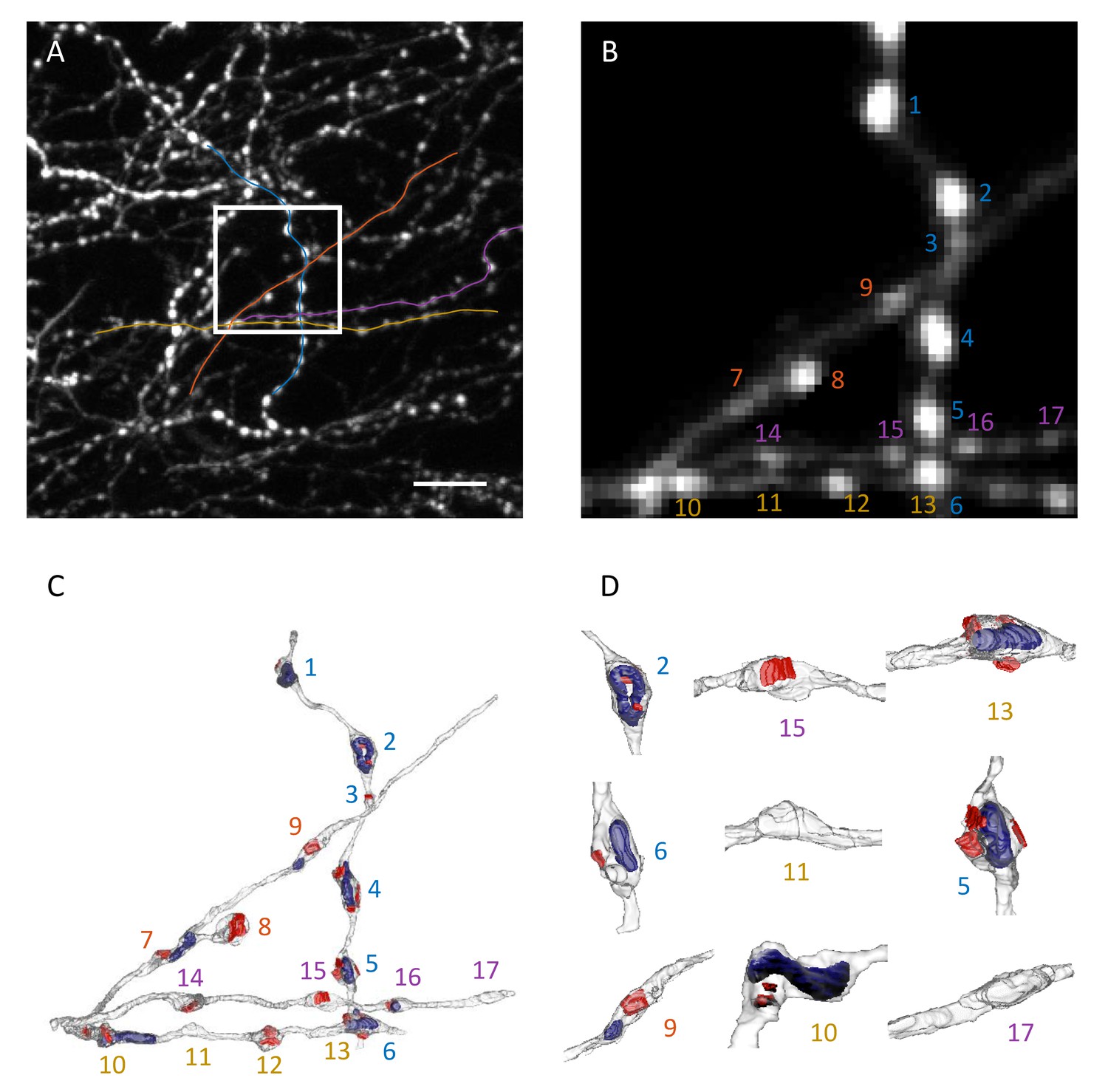
Correlative light and electron microscopy.
(A) Maximum intensity xy projection of an image stack used for CLEM analysis. White box demarcates the region imaged with EM. Colored lines are traces of four axon segments chosen for EM reconstruction. Scale bar is 10 μm. (B) Region outlined in (A) is shown at 4x magnification with background removed. (C) 3D EM reconstruction of the four axon segments shown in (B). Red areas mark PSDs, and blue volumes outline mitochondria. Most varicosities identified in EM are clearly visible in 2PLSM images (B). (D) Higher magnifications and different orientations of a subset of reconstructed varicosities shows that structural swellings on axons may or may not be associated with PSDs and/or contain mitochondria. Numbers in (B–D) enumerate distinct varicosities identified in EM.
Figure 3—video 1
Illustration of correlative light and electron microscopy analysis.
LM-based bouton detection on four axon segments is validated with 3D EM-based reconstruction of the same axons. Dots indicate putative boutons detected automatically in LM. Their size is proportional to bouton weight. Color-code is the same as in Figure 3.
Figure 4 with 1 supplement

Normalized intensity profile is correlated with axon cross-section area, while bouton weight is indicative of bouton volume.
(A–D) Top row: EM reconstructions of axons are shown next to the corresponding 2PLSM maximum intensity projections. Varicosities identified in EM are marked with grey asterisks, and putative boutons automatically detected based on the intensity profiles are marked with green asterisks. Second row: Normalized intensity profiles of the same axons plotted as functions of position along axon centerlines obtained in EM. Third row: z cross-section areas of axons, including (black) and excluding (blue) mitochondria, are well correlated with intensity profiles. These cross-sections are drawn perpendicular to the 2PLSM xy projections of the axon centerlines. Fourth row: Normal cross-section areas showing the extents of boutons (green) based on criteria described in Materials and methods. (E) Demarcated boutons shown in 3D (green). Bouton weights are highly correlated with their EM-based volumes that include (F) or exclude (G) mitochondrial volumes. Grey regions in (B) highlight two spurious peaks in the normalized intensity profile, one resulting from a close apposition of two axons and another caused by the presence of a terminal bouton. Such regions were annotated in 2PLSM images and were excluded from all analyses. In addition, bouton #7 (red box in B, F, and G) was excluded from the correlation analysis because it is directly adjacent to a branch point, which biases weight calculation.
Figure 4—figure supplement 1
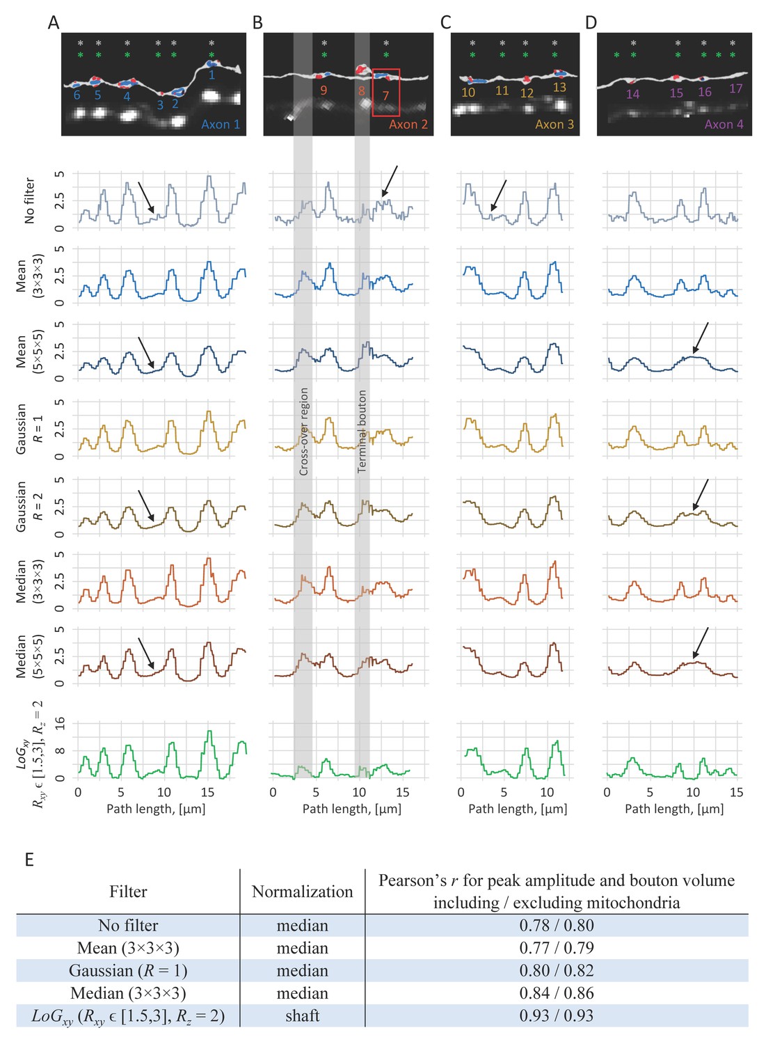
Filter type, filter size, and profile normalization can affect bouton detection and measurement.
(A–D) Comparison of axon intensity profiles obtained with different filters. Each profile is plotted as a function of position on axon trace obtained in LM. Top row: EM reconstructions and 2PLSM maximum intensity projections for the four axons included in CLEM analyses (same as shown in Figure 4). Rows 2–8 show intensity profiles of these axons generated by using raw voxel intensities along the trace, mean filters of box sizes 3 × 3 × 3 and 5 × 5 × 5, Gaussian filters [see Equation (1)] of sizes R = 1 and R = 2, and median filters of box sizes 3 × 3 × 3 and 5 × 5 × 5. Each profile was normalized by its median profile intensity. Row 9 shows multi-scale LoGxy profiles normalized by shaft intensities. In the absence of filtering, profiles appear jagged, which may lead to false positives in peak detection (arrows). On the other hand, large filters (5 × 5 × 5 and R = 2) may not resolve small boutons or closely positioned boutons (arrows). When the filter size is carefully tuned (3 × 3 × 3 and R = 1 in this case) profiles generated by various filters may appear similar to those obtained with the multi-scale LoGxy. (E) Bouton measurements based on these profiles were compared to bouton volumes measured in EM. LoGxy filter profile normalized with shaft intensity leads to both accurate bouton detection and highest degree of correlation between peak amplitudes on the profiles and bouton volumes.
Figure 5
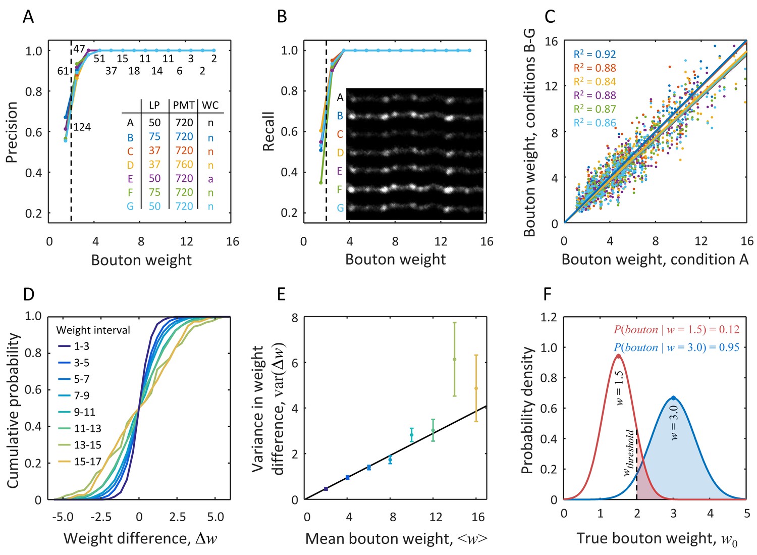
Probabilistic definition of an LM bouton based on measurement uncertainty derived from short-term imaging experiments.
The same set of axons was imaged 7 times within 80 min with various microscope settings and cranial window conditions (inset in A). Putative boutons detected based on the first imaging session (condition A) were chosen to be the gold standard. Precision (A) and recall (B) in bouton detection were measured under the remaining conditions, B-G. Both precision and recall increase with bouton weight. While for very small boutons ( < 2.0, dashed line) detection is unreliable, agreement with the gold standard is achieved across all imaging conditions in 95% of boutons with weights greater than 2.0. Numbers of boutons in the gold standard are indicated next to the data points in (A). Inset in (B) shows an example of one axon segment imaged in conditions A-G. (C) Bouton weights under different imaging conditions are plotted against the gold standard weight. Best fit lines show no significant bias for conditions B and C, however small, but significant reduction in mean bouton weight was observed in the remaining four conditions (all p < 0.03, two-sample t-test). Abbreviations used in the inset of A: LP is laser power in mW, PMT denotes photomultiplier tube voltage in Volts, and WC is cranial window condition, where ‘n’ stands for normal and ‘a’ indicates presence of a thin layer of agarose. Color code used in (A–C) is defined by the inset table in (A). (D) CDFs for differences in bouton weights across imaging conditions. Data from all conditions were pooled. Different lines show CDFs for various intervals of mean bouton weight. (E) Variance in bouton weight difference increases linearly with mean bouton weight (χ2 linear regression with , p = 0.33, α = 0.24 ± 0.01, mean ± s.d.). Error-bars indicate standard deviations obtained with bootstrap sampling with replacement. (F) Red line shows the distribution of true bouton weight for a putative bouton of measured weight = 1.5. Area under the curve to the right of = 2.0 gives = 0.12. Large putative boutons (e.g. blue curve, = 3.0) have high probability of being LM boutons.
Figure 6 with 1 supplement
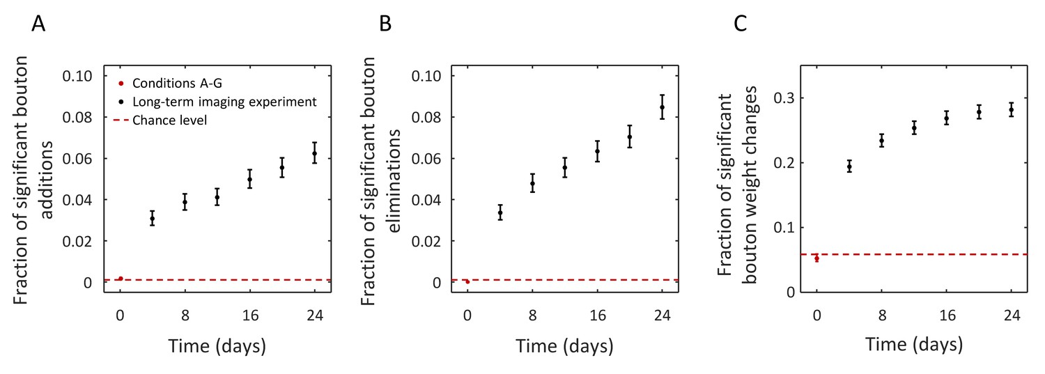
Structural change in boutons can be resolved in long-term in vivo imaging experiments despite measurement noise.
(A) Fraction of boutons that are absent on day 0 and are present at a later time with joint probability of 0.95 or greater (significant bouton addition). Red point (error-bars are too small to be visible) shows this fraction in images acquired within 80 min (conditions A-G). Black points show the results for a long-term imaging experiment. Statistically significant fraction of added boutons is detected after 4 days (interval between imaging sessions), and this fraction grows with time, consistent with the idea of gradual modification of the initial circuit. Similar trends were observed for the fractions of significant bouton eliminations (B) and significant bouton weight changes. Dashed red lines in (A–C) indicate baseline circuit changes expected from the statistical model. Error-bars indicate standard deviations based on Poisson statistics.
Figure 6—figure supplement 1
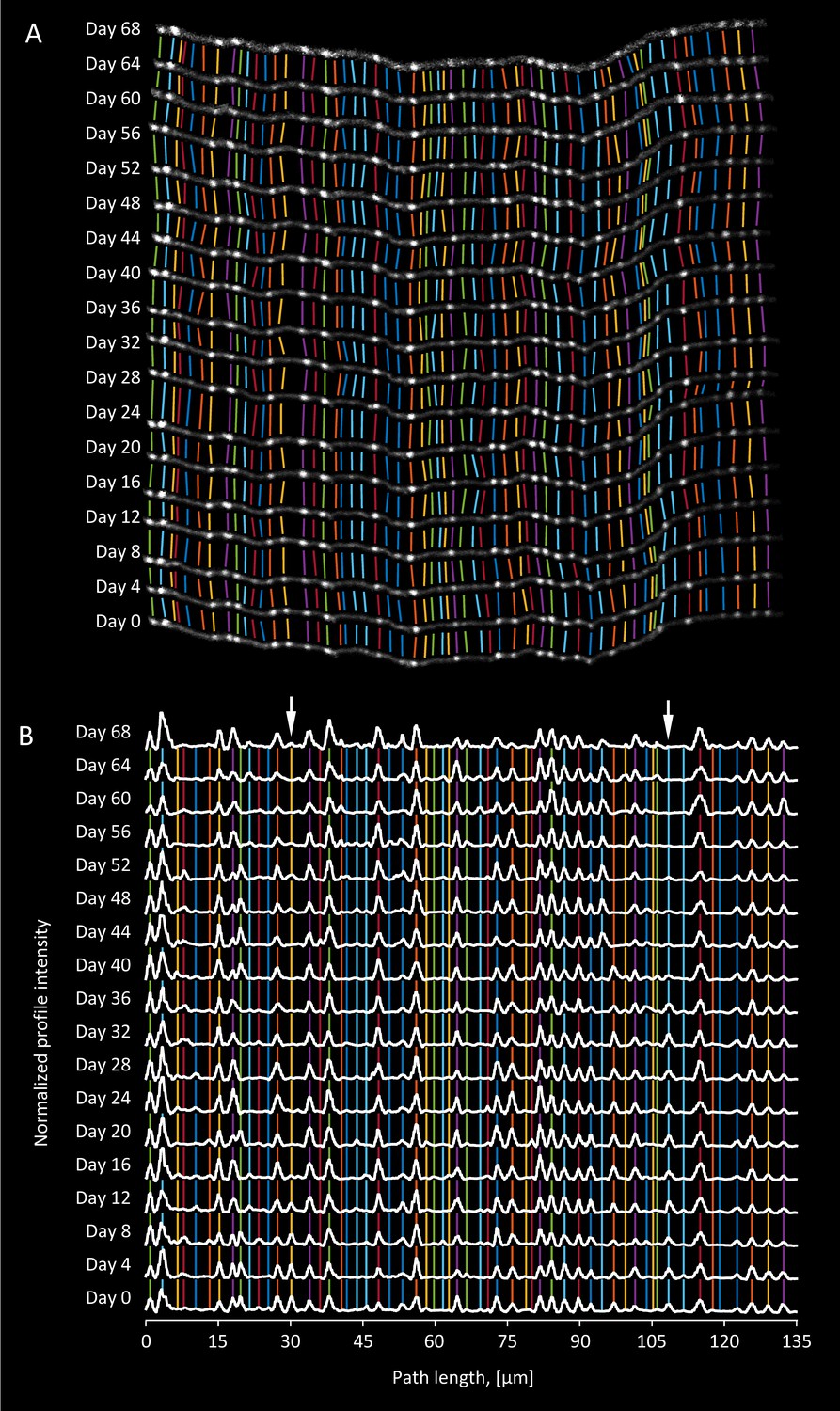
Matching boutons in time-lapse images.
(A). xy projection of an axon segment that was imaged at 4 day intervals over a period of 68 days. Image intensity in each session is normalized independently as described for intensity profiles. Colored lines link corresponding putative boutons. These lines do not always run in parallel due to small rotations of the brain, nonlinear tissue distortions, and movements of boutons. (B). Normalized and aligned intensity profiles of the axon from A (see Materials and methods for details). Arrows indicate two locations on the axon where a bouton present on day 0 was eliminated after few imaging sessions.
Tables
Table 1
Comparison of LM-based and EM measurements.
Bouton IDs match those in Figures 3 and 4. The probability that a putative bouton belongs to the category of LM boutons, was calculated according to Equation (9) with = 2.0. Bouton #8 (grey) was excluded from the analyses as it is a terminal bouton. Hyphens indicate that boutons, mitochondria, or PSDs were not detected in EM.
| 2PLSM measurements | EM measurements | |||||
|---|---|---|---|---|---|---|
| Bouton ID | Putative bouton weight, w | P(bouton | w) | Bouton volume [μm3] | Mitochondria volume [μm3] | PSD surface area [μm2] | |
| Axon 1 | 1 | 13.5 | 1.00 | 0.919 | 0.189 | 0.666 |
| 2 | 10.8 | 1.00 | 0.779 | 0.170 | 0.595 | |
| 3 | 1.98 | 0.48 | 0.093 | - | 0.371 | |
| 4 | 10.1 | 1.00 | 0.998 | 0.225 | 1.92 | |
| 5 | 8.65 | 1.00 | 0.669 | 0.139 | 1.83 | |
| 6 | 6.25 | 1.00 | 0.219 | 0.043 | 0.138 | |
| Axon 2 | 7 | 3.63 | 0.93 | 0.483 | 0.111 | 0.612 |
| 8 | N/A | N/A | 0.574 | - | 2.75 | |
| 9 | 5.57 | 1.00 | 0.372 | 0.027 | 1.28 | |
| Axon 3 | 10 | 9.54 | 1.00 | 0.632 | 0.182 | 0.645 |
| 11 | 1.99 | 0.49 | 0.102 | - | - | |
| 12 | 8.51 | 1.00 | 0.456 | - | 1.23 | |
| 13 | 10.8 | 1.00 | 0.704 | 0.161 | 1.49 | |
| Axon 4 | 14 | 5.80 | 1.00 | 0.308 | - | 0.867 |
| 15 | 4.23 | 1.00 | 0.198 | - | 0.686 | |
| 16 | 5.96 | 1.00 | 0.229 | 0.027 | 0.402 | |
| 17 | 2.85 | 0.93 | 0.140 | - | - | |
| 18 | 1.14 | 0.01 | - | - | - | |
| 19 | 2.19 | 0.65 | - | - | - | |
Additional files
-
Transparent reporting form
- https://doi.org/10.7554/eLife.29315.014
Download links
A two-part list of links to download the article, or parts of the article, in various formats.
Downloads (link to download the article as PDF)
Open citations (links to open the citations from this article in various online reference manager services)
Cite this article (links to download the citations from this article in formats compatible with various reference manager tools)
Computer assisted detection of axonal bouton structural plasticity in in vivo time-lapse images
eLife 6:e29315.
https://doi.org/10.7554/eLife.29315


