Figures and data in Exploratory search during directed navigation in C. elegans and Drosophila larva | eLife

Figures
Additional files

4 figures and 2 additional files

Figures

Figure 1 with 1 supplement

Download asset Open asset

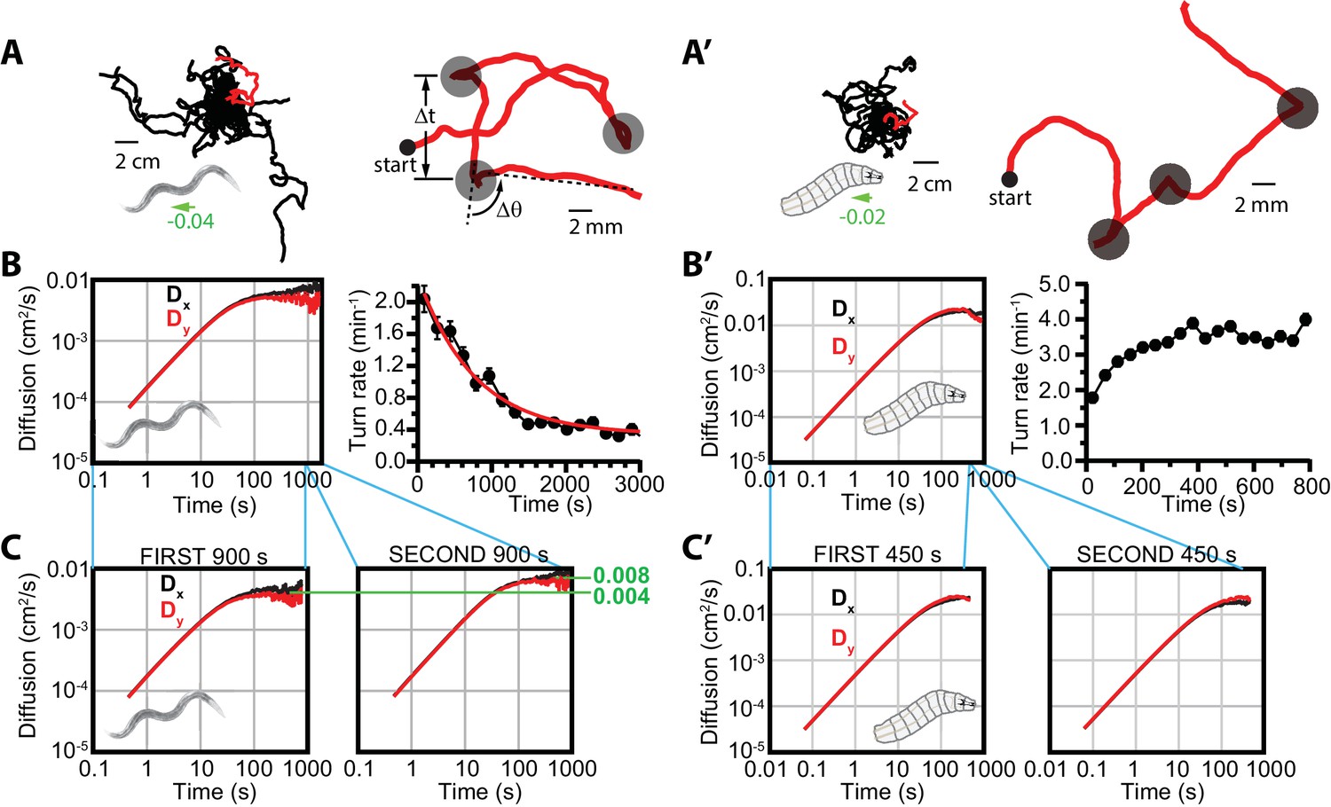
Diffusive searching in C. elegans and Drosophila larva.

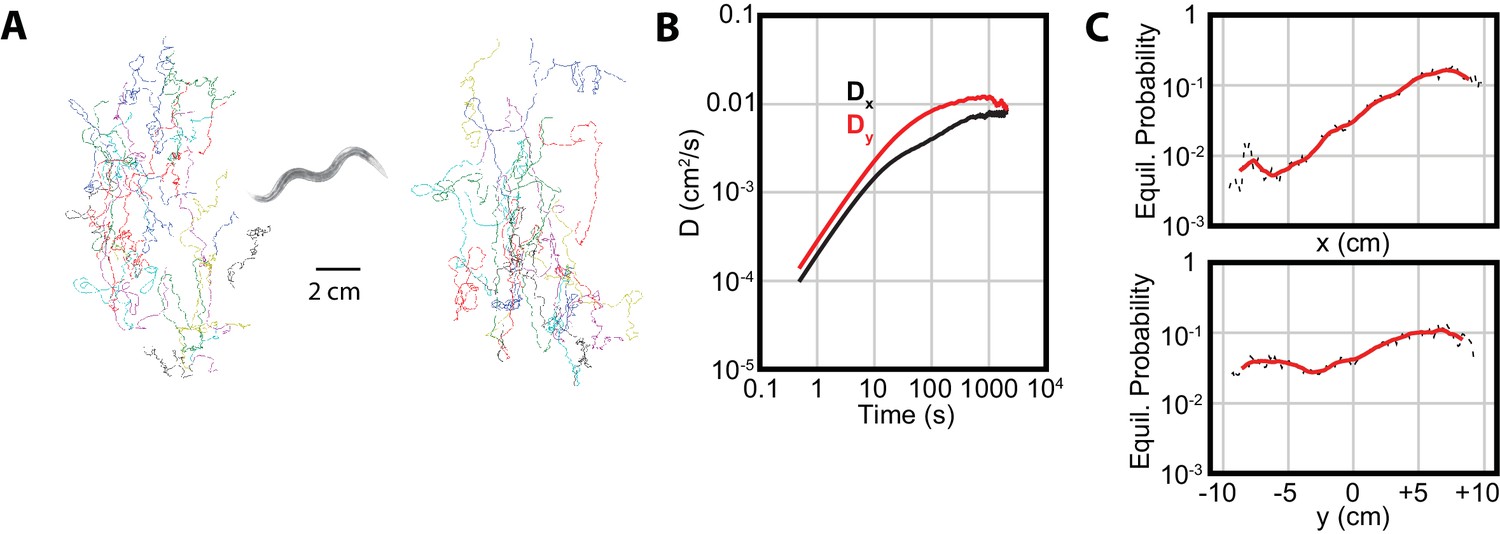
(A) Sample trajectories (left) from 18 worms under isotropic conditions, for 60 min. Tracks have been shifted to all begin at the same location for clarity. A single track (red) is magnified (right) to show the abrupt changes in crawling orientation, flagged as ‘turns’ (gray circles), with comparatively straight-crawling ‘runs’ in between. Runs are characterized by their duration $Δ t$ , and turns by their change in heading $Δ θ$ . (B) Diffusion in the $x$ - and $y$ -directions and turning rate reduction over time. Worms diffuse in both directions (left), while the rate of turning events steadily decreases over 3000 s (right); it fits an exponential decay (red) with a 765 s time constant. (C) Diffusion in the $x$ - and $y$ -directions, splitting the time window into $t < 900$ s (left) and $900 < t < 1800$ s (right). (A’) Sample trajectories from 25 Drosophila larvae navigating under isotropic conditions for 15 min. (B’) Diffusion and turning rate over time for crawling Drosophila. $D_{x}$ and $D_{y}$ reach similar values, substantially higher than C. elegans (left), and the turning rate does not show a dramatic drop, instead increasing for the first ~2 min. before stabilizing. (C’) Split $D_{x}$ and $D_{y}$ graphs covering the first ( $t < 450$ s) and second ( $450 < t < 900$ s) halves of the trajectory time, converging to similar values in each. Results for (B,C) are based on seven experiments, with 56 tracks and a total of 1608 turns. Results for (B’,C’) are based on 30 experiments, with 434 tracks and 11,294 turns. The directions of overall population drift for (A,A’) are indicated by green arrows, with the numbers indicating the dimensionless drift velocity, in this case extremely small (see Materials and methods). Error bars for (B,B’) are $\pm$ s.e.m.

https://doi.org/10.7554/eLife.30503.002

Figure 1—source data 1 Values and s.e.m. for diffusion coefficient vs. time plots: https://doi.org/10.7554/eLife.30503.004
Download elife-30503-fig1-data1-v1.zip

Figure 1—figure supplement 1

Download asset Open asset

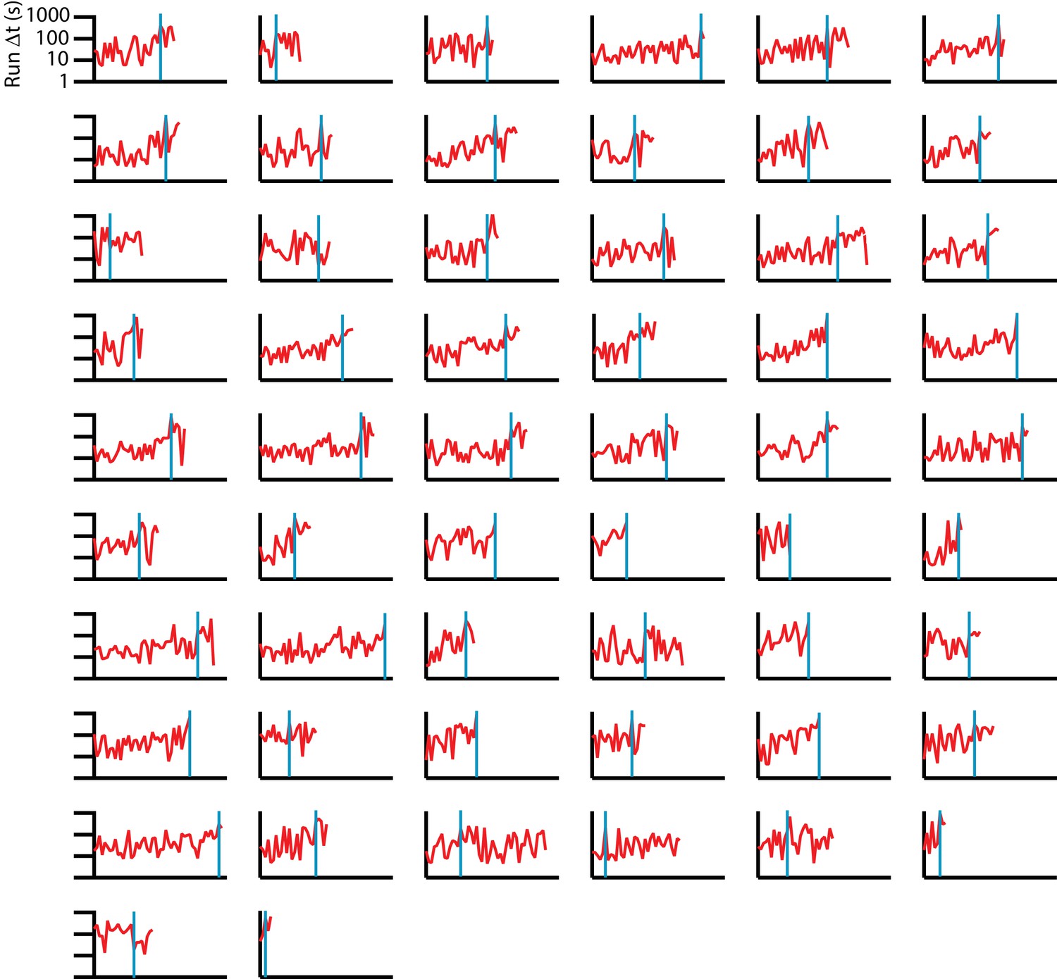
Consecutive run durations for individual C. elegans tracks under isotropic conditions.

56 sequences are shown (red), with a blue vertical line indicating the change point, found by maximizing the difference in average $Δ t$ below and above a particular time in the experiment. Change point times have a wide range, in many cases occurring near the end of trajectories, indicating a steady rise with high variance, rather than an abrupt transition in mean run duration. We note that in more than half the tracks, the difference in mean before and after the change point is less than twice the standard deviation of the data prior to the change point.

https://doi.org/10.7554/eLife.30503.003

Figure 2 with 1 supplement

Download asset Open asset

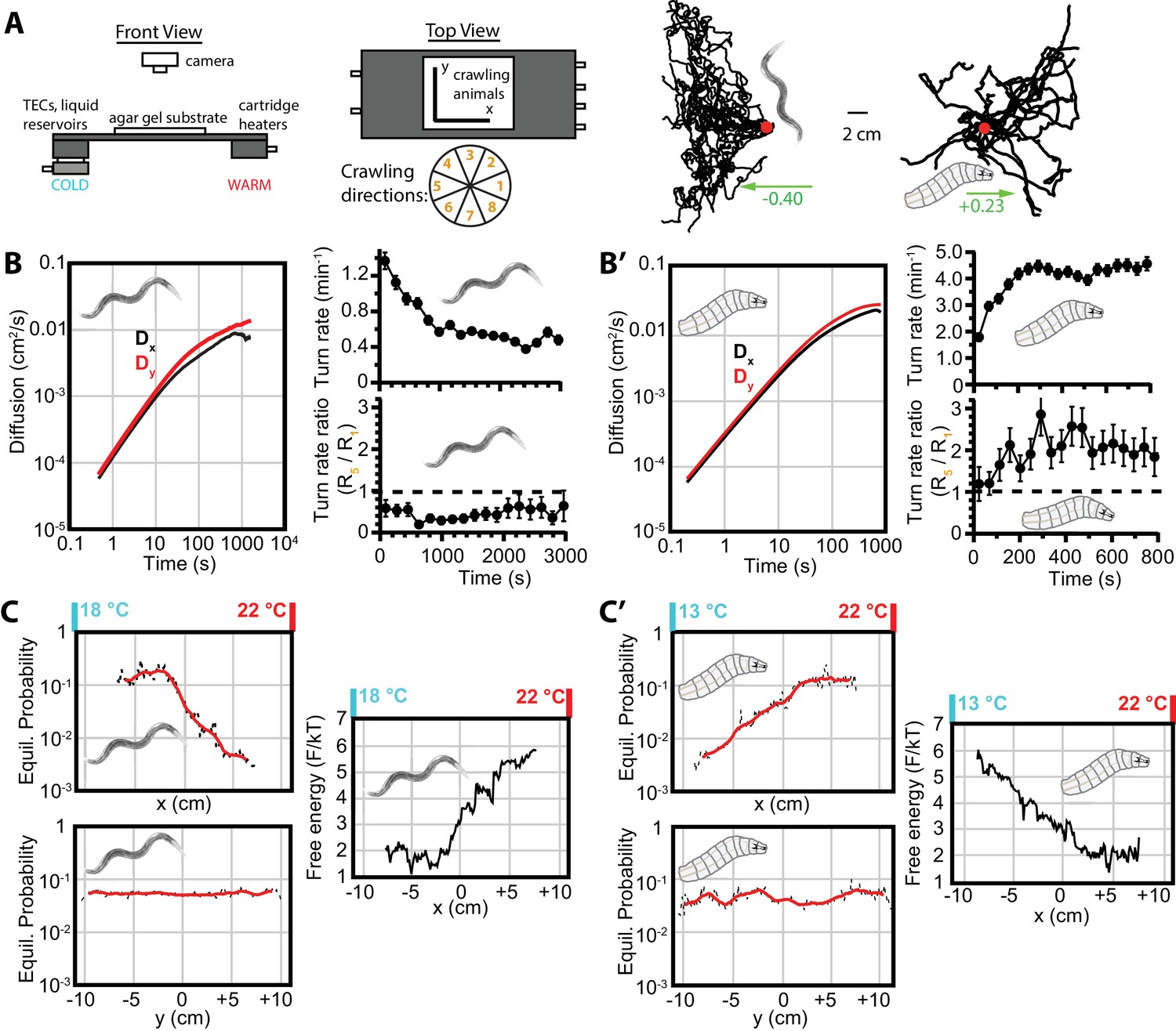
Diffusion and navigation in C. elegans and Drosophila thermotaxis.

(A) Schematic of the apparatus (left), where animals crawl atop an agar substrate while exposed to a 1D linear temperature gradient. Sample thermotaxis trajectories (right) from 18 C. elegans crawling for 60 min and 25 Drosophila crawling for 15 min, where the red dots indicate the starting position for all trajectories. Worms start at 20°C and exhibit negative thermotaxis, moving toward their 15°C cultivation temperature, while larvae start at 17.5°C and crawl away from aversive cold temperatures. The wheel indicates labels for crawling direction ranges, with octant 1 parallel to the gradient heading toward warmer temperatures and octant 5 heading antiparallel towards cooler temperatures. (B) Diffusion over time (left) in the x- and y-directions for C. elegans. $D_{y} > D_{x}$ throughout the experiment, indicating diminished, but highly significant, diffusion along the navigation direction. The average turning rate (upper right) diminishes over time, as in the Figure 1B,B’ isotropic case; the turning rate ratio $R_{5} : R_{1}$ (lower right) remains below 1 and nearly constant throughout the experiment. (C) Equilibrium probability distributions in the x (top) and y (bottom) directions (both use the same scale), extrapolated from empirical trajectories using the Markov state model (MSM). The lag time used is 750 s. Red lines are smoothed traces to guide the eye. The free-energy picture of equilibrium conditions (right), to place the analysis in context with the protein folding analysis tools employed here. Lower-free energy corresponds to higher population as $P \sim e x p (- F / k T)$ , where here $k T = 1$ . (B’) Diffusion, and turning rates for Drosophila larvae, also showing $D_{y} > D_{x}$ . The average turning rate stabilizes early, and the turning rate ratio $R_{5} : R_{1}$ , the primary behavioral modulation underlying thermotaxis, remains nearly constant. (C’) Equilibrium probability distributions for Drosophila larvae (left), and the corresponding free-energy landscape (right), determined from the MSM. Analysis is based on 30 experiments, 131 tracks, and 3061 turns for worms, and 20 experiments, 303 tracks, and 7771 turns for larvae. The directions of overall population drift for (A) are indicated by green arrows, with the numbers indicating the dimensionless drift velocity, approximately 10 times greater than for the isotropic navigation cases (see Materials and methods). Error bars are $\pm$ s.e.m. where shown; in the other cases the error bar size is smaller than the line thickness, and therefore not seen.

https://doi.org/10.7554/eLife.30503.005

Figure 2—source data 1 Values and s.e.m. for diffusion coefficient vs. time plots: https://doi.org/10.7554/eLife.30503.007
Download elife-30503-fig2-data1-v1.zip

Figure 2—figure supplement 1

Download asset Open asset

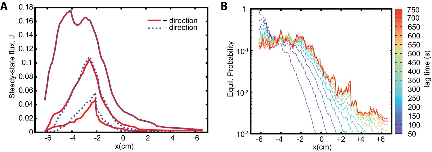
Reversability, detailed balance, and sampling intervals in the Markov state model approach.

(A) Analysis of the reversibility of the dynamics. Fluxes in positive (red) and negative (blue dashed) directions are shown. The topmost lines show $J^{+} (x)$ and $J^{-} (x)$ ; the lines are almost identical. The lowermost lines show $J_{a}^{+} (x)$ and $J_{a}^{-} (x)$ for $a = 2$ ; the lines agree, with residual difference due to statistical noise. The intermediate lines show that increasing the statistics decreases the noise and improves the agreement. (B) Equilibrium probability distribution as a function of lag time used to construct the MSM. With increasing lag time the dynamics becomes more Markovian and the determined equilibrium probabilities converge to the limiting one.

https://doi.org/10.7554/eLife.30503.006

Figure 3

Download asset Open asset

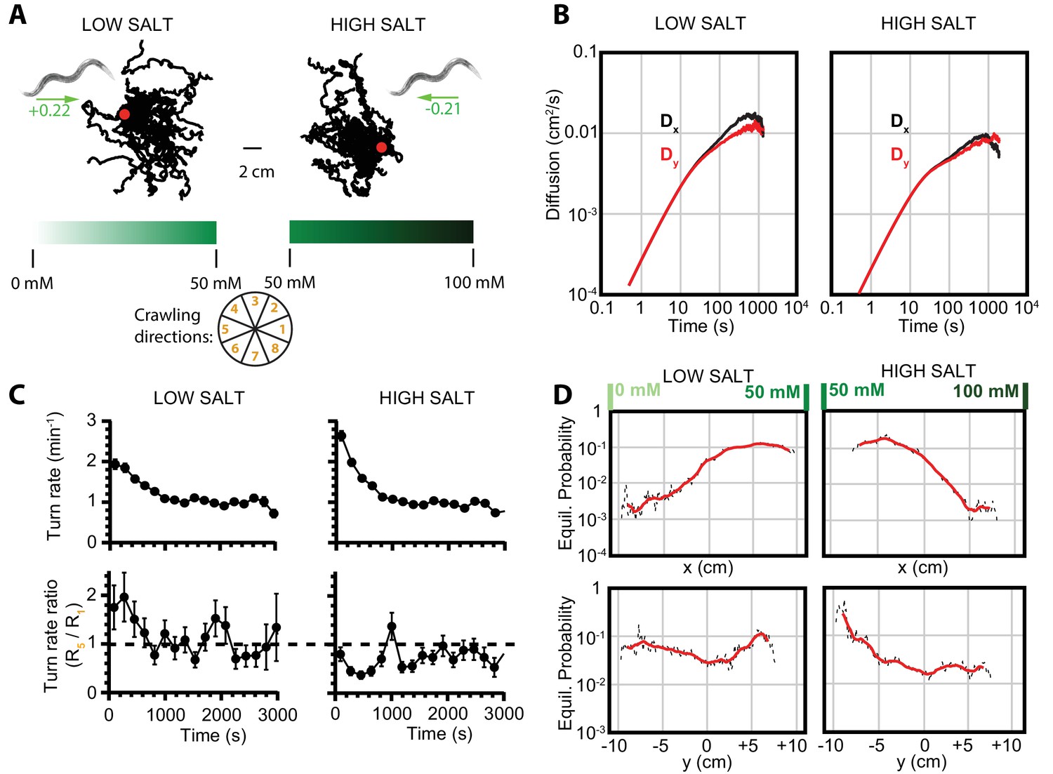
Diffusion and navigation in C. elegans salt chemotaxis.

(A) Sample trajectories (25 worms each) of crawling on an agar substrate with a salt concentration gradient increasing toward the right, under a low-salt concentration baseline (25 mM, left) and high-salt concentration baseline (75 mM, right). The wheel indicates labels for crawling direction ranges, with octant 1 pointing directly to higher salt concentrations and octant 5 directly toward low concentrations. The directions of overall population drift are indicated by green arrows, with the numbers indicating the dimensionless drift velocity, approximately 10 times greater than for the isotropic navigation cases (see Materials and methods). (B) Diffusion over time in the $x$ and $y$ directions for a low-salt baseline (left) and high-salt baseline (right). Error bars are $\pm$ s.e.m. (C) Average turning rate across all crawling directions (top) decays over time for both low and high baseline salt concentration gradients. The turning rate ratio between octant 5 (toward lower concentration) and octant 1 (toward higher concentration) does not stabilize as clearly as for thermotaxis, likely indicative of a reduced level of movement toward preferred salt conditions and a smaller data set. Error bars are $\pm$ s.e.m. (D) Equilibrium probability distributions for worms in low- (left) and high (right)-salt concentration environments, determined by using the Markov state model (MSM). Analysis is based on 14 experiments, 126 tracks, and 4422 turns for low-salt concentration, and 16 experiments, 166 tracks, and 6159 turns for high-salt concentration.

https://doi.org/10.7554/eLife.30503.008

Figure 3—source data 1 Values and s.e.m. for diffusion coefficient vs. time plots: https://doi.org/10.7554/eLife.30503.009
Download elife-30503-fig3-data1-v1.zip

Figure 4

Download asset Open asset

Isothermal tracking in C. elegans includes diffusion in the $x$ -direction.

(A) Experimental trajectories under temperature gradient conditions, with worms initially placed at their cultivation temperature of 15°C. Colors are used for the reader to distinguish between individual tracks. (B) The diffusion constants along the $x$ and $y$ directions, with $D_{y}$ dominating, but $D_{x}$ highly significant. Error bars are $\pm$ s.e.m. (C) MSM-generated equilibrium probabilities along the temperature gradient ( $x$ axis) showing the long time scale distribution of the population of worms, and perpendicular to the temperature gradient along isotherms ( $y$ axis). In $x$ , worms avoid regions with low temperatures, but freely explore regions with higher temperature; in $y$ , worms explore the axis with approximately equal probability. Analysis based on 25 experiments, with 688 tracks.

https://doi.org/10.7554/eLife.30503.010

Figure 4—source data 1 Values and s.e.m. for diffusion coefficient vs. time plots: https://doi.org/10.7554/eLife.30503.011
Download elife-30503-fig4-data1-v1.zip

Additional files

Source code 1 Scripts used in conjunction with MAGAT Analyzer software: https://doi.org/10.7554/eLife.30503.012
Download elife-30503-code1-v1.zip
Transparent reporting form: https://doi.org/10.7554/eLife.30503.013
Download elife-30503-transrepform-v1.pdf

Download links

A two-part list of links to download the article, or parts of the article, in various formats.

Downloads (link to download the article as PDF)

Open citations (links to open the citations from this article in various online reference manager services)

Mendeley

Cite this article (links to download the citations from this article in formats compatible with various reference manager tools)

Mason Klein
Sergei V Krivov
Anggie J Ferrer
Linjiao Luo
Aravinthan DT Samuel
Martin Karplus

(2017)

Exploratory search during directed navigation in C. elegans and Drosophila larva

eLife 6:e30503.

https://doi.org/10.7554/eLife.30503

Sign up for email alerts

Privacy notice