Linking time-series of single-molecule experiments with molecular dynamics simulations by machine learning

Abstract
Introduction
Results
Discussion
Methods
Data availability
References
Article and author information
Metrics

Abstract

Single-molecule experiments and molecular dynamics (MD) simulations are indispensable tools for investigating protein conformational dynamics. The former provide time-series data, such as donor-acceptor distances, whereas the latter give atomistic information, although this information is often biased by model parameters. Here, we devise a machine-learning method to combine the complementary information from the two approaches and construct a consistent model of conformational dynamics. It is applied to the folding dynamics of the formin-binding protein WW domain. MD simulations over 400 μs led to an initial Markov state model (MSM), which was then "refined" using single-molecule Förster resonance energy transfer (FRET) data through hidden Markov modeling. The refined or data-assimilated MSM reproduces the FRET data and features hairpin one in the transition-state ensemble, consistent with mutation experiments. The folding pathway in the data-assimilated MSM suggests interplay between hydrophobic contacts and turn formation. Our method provides a general framework for investigating conformational transitions in other proteins.

https://doi.org/10.7554/eLife.32668.001

Introduction

Protein folding is an important subject not only for basic research in molecular biology but also for understanding folding diseases and designing new polymeric materials (Dill and MacCallum, 2012). Transient, partially folded states are often encountered on folding pathways, and have been characterized experimentally in solution by methods such as laser temperature jumps, fluorescence labeling, and solution X-ray scattering. Mutagenesis evaluated by Φ-value analysis (Fersht and Daggett, 2002), for instance, has also provided residue-level information on transition states. Recently, state-of-the-art single-molecule (sm) measurements, single-molecule Förster resonance energy transfer (smFRET) (Chung et al., 2012; Oikawa et al., 2013) and force spectroscopy (smFS) (Neupane et al., 2016) have become powerful tools in protein-folding research, providing reliable information on transition-path (barrier-crossing process) times (Chung et al., 2012) and heterogeneity in the unfolded state (Oikawa et al., 2013). A major limitation of smFRET is that the observables are restricted to ‘low-dimensional’ structural data, such as the donor–acceptor distance. Computational modeling should help us to interpret single-molecule time-series measurements and should contribute to solving some remaining puzzles, such as the reduced solvent viscosity dependence of the transition-path times (Chung and Eaton, 2013), the internal viscosity (Chung and Eaton, 2013) and the impact of non-Markovian property (Chung et al., 2015). Theories and computational methods have been developed to extract structural information and dynamics from smFRET data (Haas et al., 2013; Hoefling et al., 2011; Matsunaga et al., 2015; Sun et al., 2016).

Molecular dynamics (MD) simulation is another powerful approach for investigating protein dynamics and folding over relatively long time periods — hundreds of microseconds or longer (Lindorff-Larsen et al., 2011). In theory, ‘low-dimensional’ smFRET measurements are interpreted in terms of the atomic structural models obtained with MD simulations. However, it is still a challenge to achieve quantitative agreement between simulation and experimental data during the entire folding process, owing not only to simulation time limitations but also to inherent force-field biases. In particular, while local interactions are well described by the current force fields, it is still difficult to reproduce energetic balances between unfolded and folded states. Indeed, Piana and coworkers showed, in their protein folding simulation study, that the folding mechanism of the villin headpiece depends substantially on the choice of force field (Piana et al., 2011). It is also known that most force fields produce unfolded states that are more compact and structured than those suggested experimentally (Piana et al., 2014). Methods based on maximum entropy (Beauchamp et al., 2014; Boomsma et al., 2014; Cavalli et al., 2013; Olsson et al., 2013 , 2014 , 2017; Pitera and Chodera, 2012; Roux and Weare, 2013) or Bayesian statistics (Bonomi et al., 2016) were recently developed for guiding simulations or models to generate ensembles that match experimental ensemble-averaged observations.

Exploiting time-series data from single-molecule experiments is another way to link simulation with experiment and has several advantages over the ensemble-average based approaches: (i) more latent states can be uncovered by inferring states from their historical evolution than from their static ensembles (Li et al., 2008; Matsunaga et al., 2015; Schuetz et al., 2010); (ii) the transition state can be uniquely identified as a dynamic bottleneck by following the actual dynamics. However, the time-scale gap between experiment and simulation previously hampered the direct use of time-series analysis methods in other disciplines, such as data assimilations that are based on the sequential Monte Carlo method (Matsunaga et al., 2015).

Here, we develop a new approach for single-molecule time-series data based on the Markov state model (MSM) (Pande et al., 2010), a statistical model that approximates dynamics by memory-less probabilistic transitions between discrete conformational states. In MSM, the probability of transition from the discrete state i to state j in a lag time of τ is described by a transition-probability matrix $T (τ) = {T_{i j} (τ)}$ . $T (τ)$ can be estimated from a set of short simulations instead of a single long simulation. Therefore, MSM is often used to generate long-time dynamics (Silva et al., 2014) whose time-scale is comparable to those of experimental measurements (Feng et al., 2016; Noé et al., 2011; Snow et al., 2002). However, estimation of $T (τ)$ is largely dependent on the simulation force-fields, which may have uncertainties or biases for certain conformations (Olsson et al., 2017). To overcome this problem, we propose to "refine" $T (τ)$ using high-resolution measurement of single-molecules as time-series data. Specifically, we use a machine-learning approach to estimate $T (τ)$ between hidden Markov states from low-dimensional time-series data (Bishop, 2006). To distinguish the original $T (τ) (= T_{simulation} (τ))$ , we refer to the refined $T (τ)$ as $T_{experiment} (τ)$ in this paper.

We propose a two-step procedure in our machine-learning approach, which links simulations and single-molecule experiments (Figure 1). (i) Supervised learning step. We first construct an initial MSM from a raw set of simulation data. After defining discrete conformational states by clustering the trajectory snapshots, $T (τ) = T_{simulation} (τ)$ is estimated directly by counting transitions between the discrete states in the simulation trajectories. This step is the same as conventional MSM (Pande et al., 2010). (ii) Unsupervised learning step. Using $T_{simulation} (τ)$ as an initial estimate, we perform hidden Markov modeling (Bronson et al., 2009; McKinney et al., 2006; Okamoto and Sako, 2012; Pirchi et al., 2016; Rabiner and Juang, 1986; Schröder and Grubmüller, 2003) to refine the initial MSM using single-molecule measurement time-series data. $T (τ)$ is optimized so that the "refined" or data-assimilated MSM with $T_{experiment} (τ)$ can reproduce the time-series data most accurately.

Figure 1 with 1 supplement see all

Download asset Open asset

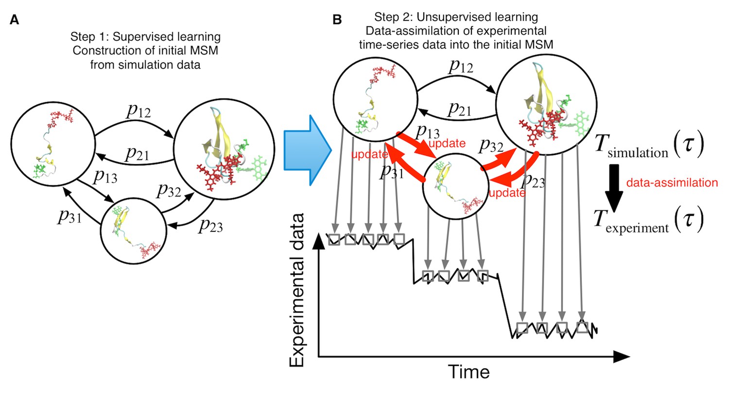
Schematic of proposed semi-supervised learning approach.

(A) Our proposed approach comprises two steps. As the first step, an initial Markov State Model is constructed only from simulation data by simply counting transitions between conformational states. (B) In the second step, transition probabilities (depicted by arrows) are updated through unsupervised learning from experimental time-series data.

https://doi.org/10.7554/eLife.32668.002

We applied this procedure to the folding dynamics of the formin-binding protein (FBP) WW domain, a 37-residue three-stranded β-sheet protein. In the construction of the initial MSM, extensive MD simulations of a dye-labeled WW domain were performed for an aggregated time of ~400 μs. Although there are a number of folding simulation studies for the FBP WW domain and its homologs (Ensign and Pande, 2009; Freddolino et al., 2008; Karanicolas and Brooks, 2003; Zanetti-Polzi et al., 2017; Zhou et al., 2014), this may be the first folding simulation to use FRET dyes. High time-resolution smFRET measurements of WW domain folding and unfolding dynamics were used for the unsupervised learning (Chung et al., 2012). The data were previously measured to resolve the durations of the folding and unfolding transitions with microsecond resolution by Chung and coworkers (Chung et al., 2012). The initial and data-assimilated MSM showed different folding pathways and transition-state ensembles of WW domains. An independent mutation experiment with Φ-value analysis (Fersht and Daggett, 2002) validated the data-assimilated MSM. We discuss our time-series analysis method in the context of machine-learning theory and its applicability to conformational transitions in other biomolecules.

Results

Single-molecule FRET measurements

SmFRET experiments were carried out by Chung and coworkers, and details for the experiments are given in Chung et al., 2012. Here we summarize the essential experimental setups necessary for our machine-learning procedure. Photon trajectories were measured for the FBP WW domain with donor (Alexa 488) and acceptor (Alexa 594) fluorophores attached to the terminal residues in the protein. In order to improve the time resolution of the smFRET data, Chung and coworkers illuminated the protein with a very high intensity laser (10 kW/cm²), increasing the number of photons observed per time (~650 photons/ms) (Chung et al., 2012). Photon color, either donor green or acceptor red, and the absolute time of arrivals were recorded within ~0.5 ns. Each photon trajectory was split into folded and unfolded segments by finding the photon interval with the maximum transition probability (Gopich and Szabo, 2009). The final set of smFRET photon sequences comprises 527 trajectories, each of which contains a single folding or unfolding event.

Molecular dynamics simulations

A dye-labeled WW domain was built in silico for MD simulations (Figure 1—figure supplement 1). Starting from the NMR structure of the WW domain (PDB code: 1E0L [Macias et al., 2000]), we made the same substitution mutation W30A as in the experiments (Chung et al., 2012), and the terminal residues were labeled with donor (Alexa Fluor 488) or acceptor (Alexa Fluor 594) dyes by using the AMBER-DYES package (Graen et al., 2014).

We conducted eleven simulations of length 25.6 μs in the NVT ensemble (370 K) from the unfolded structures. By monitoring the fraction of native contacts, Q, we observed folding events in four trajectories out of the eleven (Figure 2—figure supplement 1A). Also, six simulations of length 10 μs and four simulations of 14 μs were performed from the folded structure. In these ten trajectories, we observed seven unfolding events. Our simulations, thus, sampled intermediate regions between the unfolded and folded states sufficiently for construction of an initial MSM. The simulation length is ~400 μs in total.

Clustering of sampled structures in MD simulations

For the MSM construction, we chose a two-dimensional (2-D) space spanned by the native contact Q and the expected FRET efficiency ε. The value of ε is calculated from the distance r between donor and acceptor dyes using the Förster theory, $ε = 1 / [1 + {(r / R_{0})}^{6}]$ , where R₀ is the Förster radius (see 'Methods' for details). Here, Q is chosen because it is historically known to be the best reaction coordinate to describe a folding process. Also, ε is employed for comparison with smFRET data as well as for differentiating compact and elongated structures. Figure 2A shows a scatter plot of the sampled conformations in the MD simulations. Expected FRET efficiency ε successfully resolves the elongated unfolded states and compact states, whereas ε fails to discriminate the folded state (corresponding to Q ~ 0.7–1.0 and ε ~ 0.7–1.0) from the compact unfolded state (Q ~ 0.0–0.3 and ε ~ 0.7–1.0) without the help of Q. This suggests that approaches that are based on ensemble average may have a difficulty when the histogram of ε is used to add biases to the protein in MD simulations.

Figure 2 with 9 supplements see all

Download asset Open asset

Sampled conformations from simulations and Markov state models constructed in Q and expected FRET efficiency space.

(A) Scatter plot of sampled conformations from the aggregated trajectories. Representative structures from folded, compact unfolded, and elongated states are shown. Donor and acceptor dyes are colored green and red, respectively. (B) Cluster centers used for constructing the Markov state model are plotted with circles. (C) Initial Markov state model constructed from simulation data only. Node areas are proportional to the equilibrium populations, and edge line widths are proportional to the transition probabilities. (D) Data-assimilated Markov state model after unsupervised learning from smFRET photon-count sequences. Edges with transition probabilities of less than 0.01 are not shown for visual clarity.

https://doi.org/10.7554/eLife.32668.004

Sampled conformations were clustered into discrete states in the 2-D space (cluster centers are shown in Figure 2B). Regular spatial clustering was applied to partition the space in an equidistant manner regardless of the population size (Senne et al., 2012). This spatial clustering is essential in this study because relatively minor populations can have high probabilities after the refinement of the initial MSM with the help of experimental time-series data.

In order to obtain structural insights, we calculated both the mean and the variance of the donor-acceptor distance r for each state. Figure 2—figure supplement 2 shows samples plotted in the 2D space spanned by Q and r. There are distance gaps between states, which are supportive of the Markovian assumption. Large standard deviations are observed in the case of small donor-acceptor distances. This results from the lower spatial resolution in FRET efficiency ε when ε is not close to 0.5 (e.g., states with ε ~ 1 cover r = 0-30 Å) as discussed in the information-binning study by Watkins and Yang (2004).

Construction of an initial MSM as the supervised learning step

MSM has two tunable parameters: the number of discrete states and the lag time τ for $T (τ)$ . Theoretically, increasing the number of discrete states and/or the lag time will produce a MSM with the least discretization error (Prinz et al., 2011), while a large number of discrete states or a longer lag time will decrease the number of samples for estimation, resulting in large statistical errors (the so-called bias-variance tradeoff) (McGibbon et al., 2014). Thus, it is common to make the number of discrete states and the lag time as small as possible, even though it compromises the accuracy of the model. Here, we examined various numbers of discrete states for MSM by calculating implied time scales (Schwantes and Pande, 2013). The ith implied time scale t_i of a MSM with $T (τ)$ is given by

t_{i} = - \frac{τ}{\ln λ_{i}},

where λ_i is the ith eigenvalue of $T (τ)$ . As the implied time scales are always underestimated relative to their true values, the slower time scales are indicative of smaller discretization errors. The implied time scales were calculated for various numbers of clustered states as a function of the lag time τ (Figure 2—figure supplement 3A). We found that the converged values of the slowest implied time scale (related to folding dynamics) successfully reproduce the time scale of folding (~5 μs) in the MD data when the number of states is larger than 80 (Figure 2—figure supplement 3B). From these observations, we chose 87 states by adjusting the cluster radius (0.08) in the regular spatial clustering.

A lag time of τ = 200 ns was chosen as a minimum time scale to achieve converged implied time scales. Note that the number of states chosen here is an order of magnitude fewer than those in other MSM studies. It is well known that the RMSD metric requires a larger number of discrete states in MSM, whereas well-defined metrics that are based on slow motions or smooth coordinates (such as contact-maps [Kellogg et al., 2012], or coordinates extracted by time-structure-based independent component analysis [Schwantes and Pande, 2013]) require a smaller number of states. A long lag time of τ = 200 ns also helps the MSM to satisfy the Markov assumption as well as improving FRET photon-count statistics in the next unsupervised learning step.

Figure 2C shows a graphical representation of the initial MSM constructed only from MD simulation data. The node areas are proportional to the equilibrium populations, and the edge line widths are proportional to the transition probabilities, $T_{i j} (τ)$ . The MSM seems to overemphasize compact unfolded states (Q ~ 0.0–0.3 and ε ~ 0.7–1.0), which results from biases of the force-field parameters not only for proteins (Best et al., 2014; Piana et al., 2014) but also for FRET dyes (Best et al., 2015).

Refinement of transition probabilities as the unsupervised learning step

In the unsupervised learning, the total log likelihood function of all smFRET photon-counting sequences $l n L (T (τ)) = \sum_{k} l n L_{k} (T (τ))$ is maximized by optimizing $T (τ)$ . First, we treated smFRET data as N independent photon-counting sequences in discretized time windows. Each sequence O_k = ${o_{1}^{(k)} \dots o_{I}^{(k)}}$ consists of a set of donor and acceptor photon counts $o_{i} = {N_{D}^{(i)}, N_{A}^{(i)}}$ detected in ith time window. I is the number of time windows and 200 ns was chosen for the photon-counting time-window width as well as for the lag time τ of MSM. The likelihood function $L_{k} (T (τ))$ is then defined as a probability to observe the kth smFRET photon-counting sequence O_k with a given $T (τ)$ (Gopich and Szabo, 2012):

L_{k} (T (τ)) = p (O_{k} | (T (τ))) = \sum_{s_{1} = 1}^{M} \dots \sum_{s_{I} = 1}^{M} p (s_{1}) h (o_{1} | s_{1}) \prod_{i = 2}^{I} p (s_{i} | s_{i - 1}) h (o_{i} | s_{i}) .

M is the number of discrete states in MSM, and s_i denotes MSM’s state at the ith time window. $p (s_{i} | s_{i - 1}) = T_{s_{i - 1} s_{i}} (τ)$ is the transition probability from state s_i-₁ to state s_i. $p (s_{1})$ is the equilibrium probability of being in state s₁. $h (o_{i} | s_{i})$ is the probability of observing donor and acceptor photon-counts $o_{i} = {N_{D}^{(i)}, N_{A}^{(i)}}$ given state s_i.

By maximizing the above likelihood function, we obtained the data-assimilated MSM with the optimized $T (τ) = T_{experiment} (τ)$ , which matches with the smFRET time-series data. Figure 2D shows that the data-assimilated MSM differs from the initial MSM. In the data-assimilated MSM, the compact unfolded state (Q ~ 0.0–0.3 and ε ~ 0.7–1.0) disappears due to a minor population with high ε in the smFRET data (see Figure 3B), while an elongated unfolded region (Q ~ 0.0–0.2 and ε ~ 0.5–0.6) is stabilized. As noted, this may reflect the biases of the force-field. Also, the different solvent conditions between the simulation (TIP3P water molecules) and the smFRET experiment (denaturant concentration) may affect the unfolded state distribution (Zheng et al., 2016). Interestingly, as another stable region, the folded state (Q ~ 0.8 and ε ~ 0.6–0.8) appears instead of other states with the same ε.

Figure 3 with 1 supplement see all

Download asset Open asset

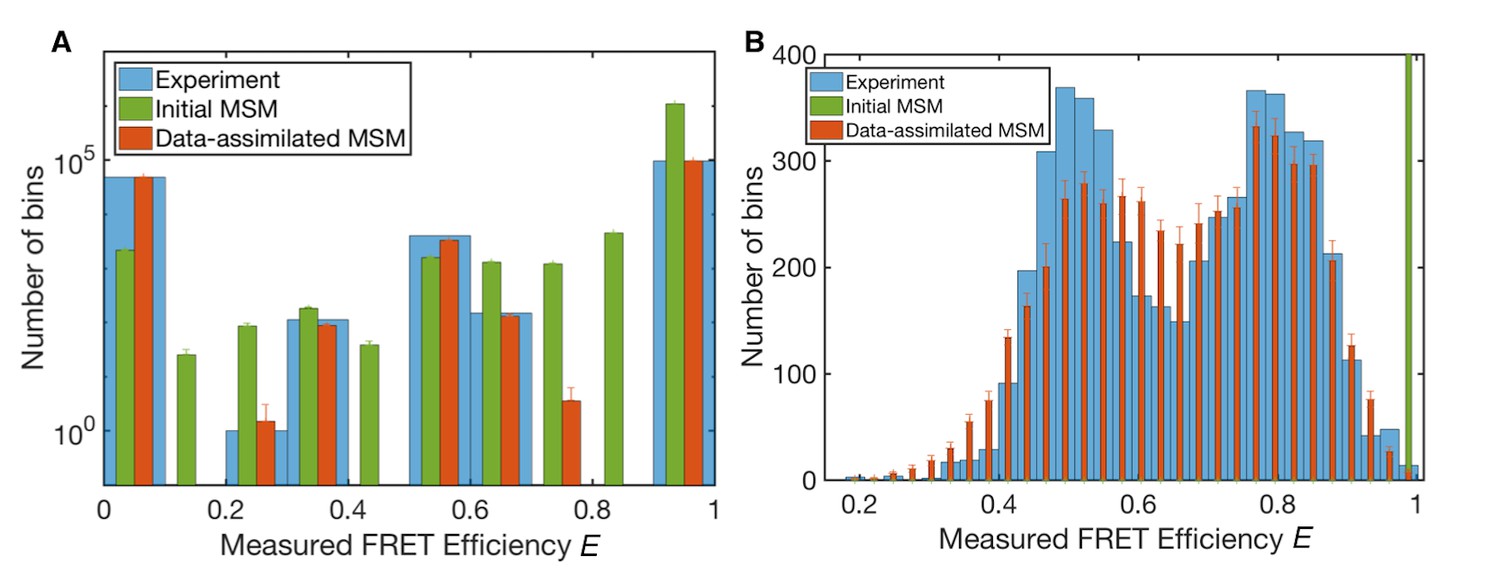
Measured FRET efficiency histograms.

(A) Measured FRET efficiency histograms calculated from donor and acceptor photons in the single-molecule FRET data with a time-window of 200 ns width, and those generated from initial and data-assimilated Markov state models. The measured FRET efficiency is defined as the ratio of the acceptor photon counts to the total number of photons (E = *N_A*/(*N_A +N_D*)). Error bars indicate standard deviations in ten realizations of photon sequences for both models. (B) Measured FRET efficiency histograms calculated with a time-window of 50 μs.

https://doi.org/10.7554/eLife.32668.014

We compared the transition probabilities $T_{i j} (τ)$ of the two MSMs (Figure 2—figure supplement 4). Figure 2—figure supplement 4A shows the implied time scales of the MSMs. We can see that the slowest time scale increases from 2.6 μs to 100 μs after the hidden Markov modeling. These time scales are related to folding/unfolding transitions of WW domain in both cases. Simulation time scale is faster than that in experiments because of the lower viscosity of the TIP3P water model (Mahoney and Jorgensen, 2001) compared to those of pure water and the viscogen added in the smFRET experiment (Chung et al., 2012). This gap was improved by the information from the smFRET data. In Figure 2—figure supplement 4B, $T_{i j} (τ)$ are directly compared in a scatter plot where each $T_{i j} (τ)$ is colored using the FRET efficiency ε of state i before transition. $T_{i j} (τ)$ from states with high FRET efficiencies are correlated with each other. This means that $T_{i j} (τ)$ related to compact states derived from MD simulations are consistent with the smFRET data. By contrast, $T_{i j} (τ)$ from states with middle or low FRET efficiencies are less correlated. This means that the hidden Markov modeling mainly updated $T_{i j} (τ)$ of elongated states.

Reproducibility of experimental data

Figure 3 shows histograms of the ‘measured’ FRET efficiency E of the original smFRET data and those generated by the initial and data-assimilated MSMs (see 'Methods' for emulation or stochastic simulation of smFRET data). The measured FRET efficiency E is calculated from the numbers of photons emitted from donor and acceptor dyes in a certain time window, N_D and N_A, respectively. It is defined by the ratio of donor photon counts to total photon counts, E = N_A/(N_A + N_D). E is calculated from measured photons in a time window whereas ε is calculated from the donor-acceptor distance of each instantaneous structure. In Figures 3A, 200 ns time-windows were used for photon counts. The data-assimilated MSM produced a histogram close to that found with original smFRET data (the mean squared error between the normalized histograms is $3.7 \times 10^{- 5}$ ), confirming the reliability of the optimized parameters obtained by machine learning.

We also calculated the observed FRET efficiency E with 50 μs time windows (Figure 3B), which corresponds to the folding time-scale observed in the smFRET data (Chung et al., 2012). The histogram of the original smFRET data has double peaks, corresponding to unfolded and folded states, respectively. The initial MSM, however, only shows a single sharp peak at high FRET efficiency because of overemphasis of compact conformations (Best et al., 2014). The data-assimilated MSM successfully reproduces the double peaks of the histogram of the original data. The histogram of the data-assimilated MSM seems smoothed compared to that obtained experimentally, presumably because of the accumulation of photon-counting noise using 200 ns time-windows.

Folding mechanisms of the FBP WW domain

To quantify the difference between the initial and data-assimilated MSMs, we calculated p_fold by applying transition-path theory (Metzner et al., 2009; Noé et al., 2009) (Figure 4A and B). p_fold is the probability of undergoing a folding transition defined for each state. States with p_fold >0.5 are kinetically closer to the folded state, whereas those with p_fold <0.5 approximate the unfolded state. Those with p_fold = 0.5 define the transition-state ensemble. The calculated p_fold tends to depend only on Q for the initial MSM (Figure 4A), as corroborated by a previous analysis of folding simulation data for various proteins (Best et al., 2013). On the other hand, p_fold of the data-assimilated MSM depends on ε as well as Q, suggesting that not only Q but also compactness needs to be factored into the folding mechanism (Figure 4B). p_fold was mapped onto the RMSDs of hairpins 1 and 2 of the native structure (Figure 4C and d). In the initial MSM, the transition-state region (p_fold = 0.4–0.6) is located in a rather compact region where the formation of both hairpins 1 and 2 can be just discerned (Figure 4E). In the data-assimilated MSM, the transition-state ensemble presents only hairpin 1 (Figure 4F). This is consistent with a mutagenesis experiment, where mutations in hairpin 1 produce large Φ-values (Petrovich et al., 2006), implying that formation of hairpin 1 contributes energetically to the transition-state ensemble.

Figure 4 with 1 supplement see all

Download asset Open asset

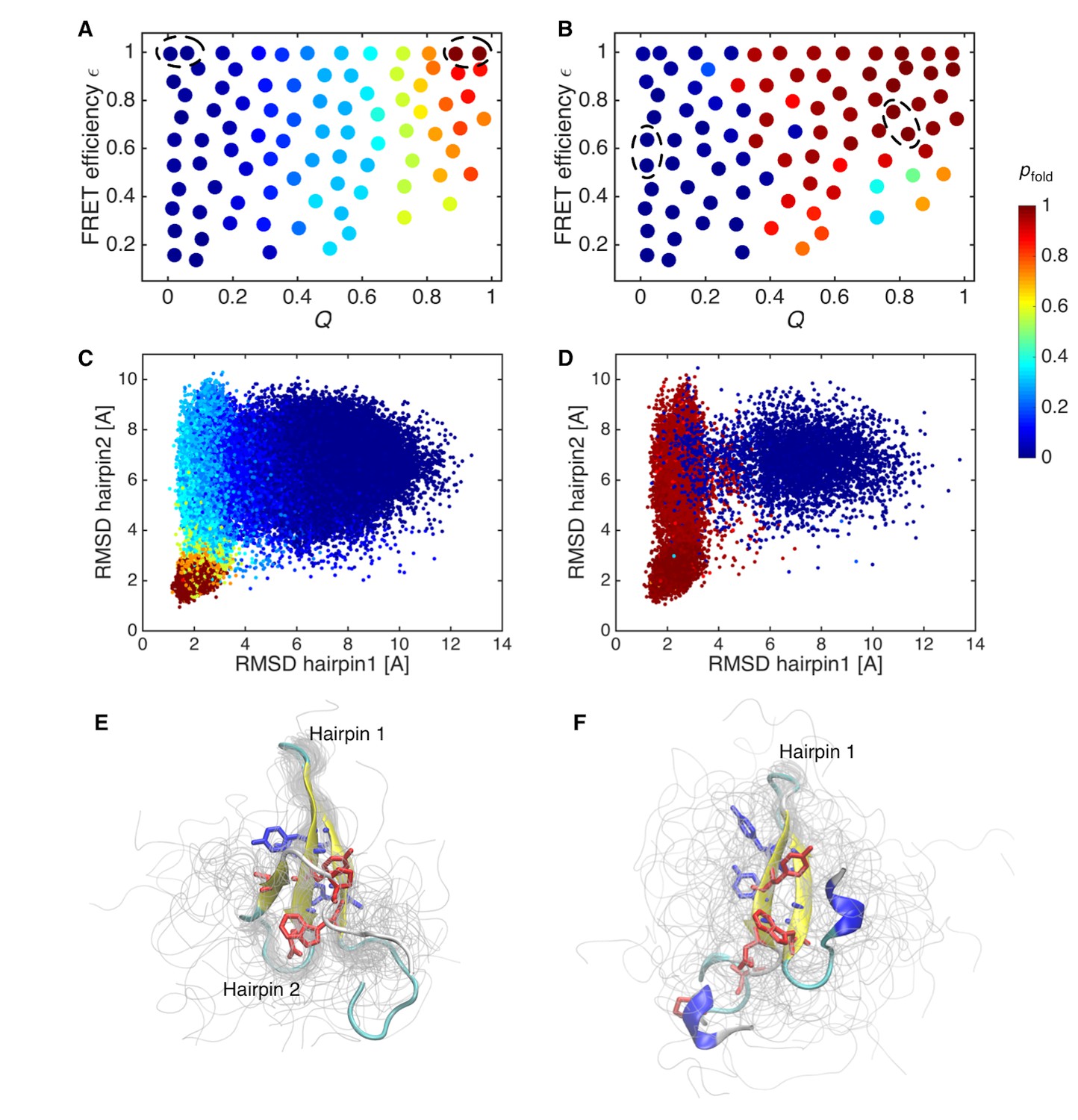
Probability of folding, p_fold, and transition state ensemble.

(A) Probabilities of folding, p_fold, mapped onto the states of initial Markov state model. (B) p_fold for data-assimilated Markov state model. The unfolded and folded states used for the calculation (source and sink in the context of the transition path theory, respectively) are indicated by circles. (C) Trajectory snapshots in the the RMSDs of hairpins 1 and 2 from their native structures are colored by p_fold for the initial Markov state model. (D) Trajectory snapshots of the data-assimilated Markov state model. (E) Structures of the transition state ensemble in the initial Markov state model which correspond to p_fold = 0.4–0.6. (F) The transition state ensemble in the data-assimilated Markov state model. Two hydrophobic cores that project below and above the plane of the sheet, core 1 (Trp8, Tyr20, Asn22, Thr29, Pro33, shown in red) and core 2 (Thr9, Tyr11, Tyr 19, Tyr21, shown in blue) are represented by sticks.

https://doi.org/10.7554/eLife.32668.016

The flux of folding trajectories can be decomposed into individual pathways for both models (Figure 5A and B). The decomposition extracts a set of pathways along with their fluxes. The dominant pathways with large fluxes provide the statistically probable order of events during folding. The figures show that folding pathways with largest fluxes contribute 50% of the total flux. In the data-assimilated MSM (Figure 5B), the formation of hydrophobic side-chain cores (core 1 consists of Trp8, Tyr20, Asn22, Thr29 and Pro33, and core 2 consists of Thr9, Tyr11, Tyr 19 and Tyr21) stabilizes the β-sheet structure in hairpin 1. The increased stability of hairpin 1 seems to guide the formation of the second hairpin (hairpin 2) by the inter-strand hydrophobic interactions. Again, this scenario is consistent with site-directed mutagenesis experiments for FBP (Petrovich et al., 2006) and the homologous Pin WW domains (Jäger et al., 2001). These experiments implied that interactions between conserved hydrophobic residues contribute to the stability of only the native state and not to the transition state ensemble. Previous simulation studies have suggested the existence of register-shifted structures as trapped (NoeNoé et al., 2009) or intermediate (Mu et al., 2006) states, whereas in the data-assimilated MSM, such states were rarely observed. Hairpin 1 formation as a rate-limiting step together with the paucity of register-shifted states in the data-assimilated MSM are consistent with the scenario of the Wako-Saitô-Muñoz-Eaton (WSME) model (Muñoz et al., 1997; Wako and Saitô, 1978), which postulates that the formation of a local turn is a bottleneck for β-sheet formation. Interestingly, hairpin 2 formation is driven by a hydrophobic collapse (Dinner et al., 1999) in the data-assimilated MSM. This implies that the interplay between turns and hydrophobic clusters has an important role in the formation of multiple hairpins in β-sheet proteins.

Figure 5

Download asset Open asset

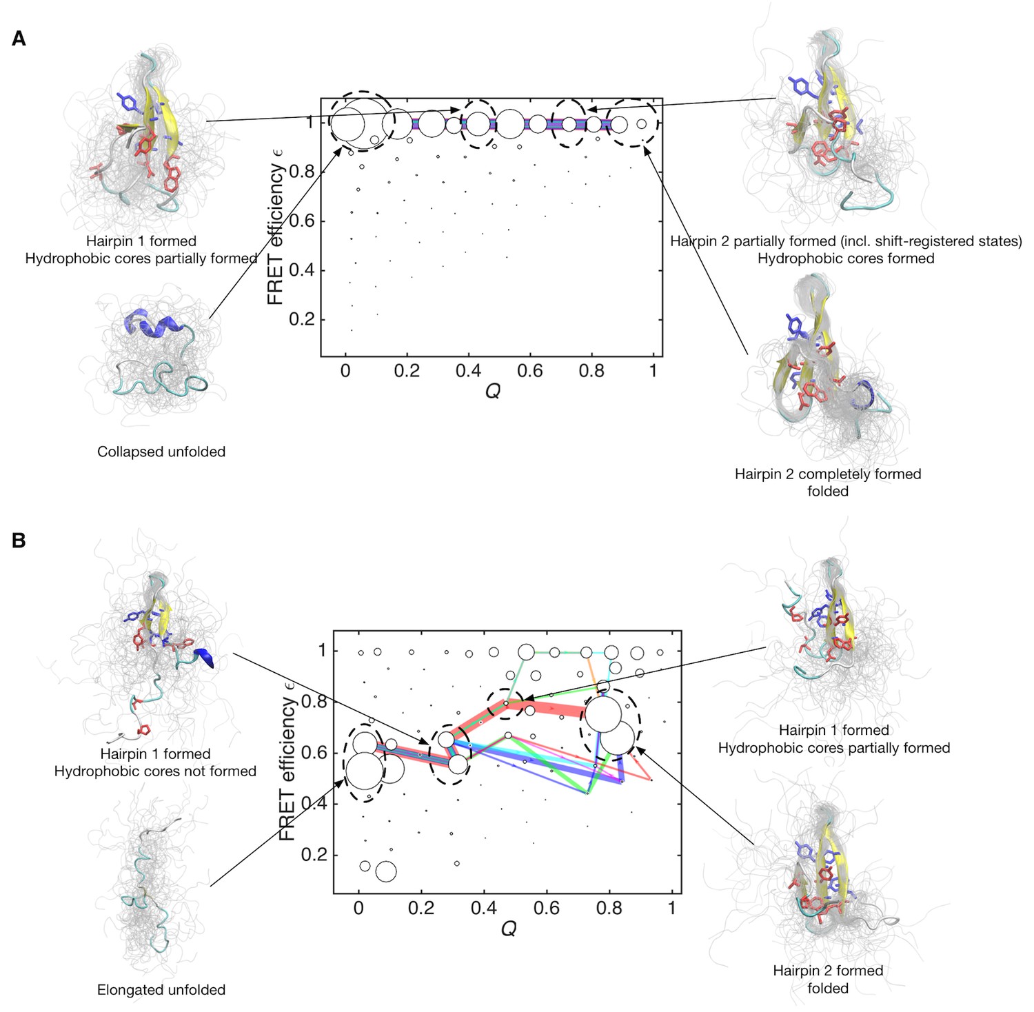
Folding pathways for initial and data-assimilated Markov state models.

(A) Folding flux of the initial Markov state model was decomposed into individual folding pathways. Folding pathways with largest fluxes contributing 50% of the total flux are superimposed in different colors. In this case, all of the pathways are located at expected FRET efficiency ε ~ 1 with different step size in the Q axis. Line widths are proportional to fluxes. Structures of representative states are shown. Two hydrophobic cores that project below and above the plane of the sheet, core 1 (Trp8, Tyr20, Asn22, Thr29 and Pro33, shown in red) and core 2 (Thr9, Tyr11, Tyr 19 and Tyr21, shown in blue) are represented by sticks. (B) Folding pathways with largest fluxes contributing 50% of the total flux are shown for the data-assimilated Markov state model.

https://doi.org/10.7554/eLife.32668.018

In terms of the theory of the coil-globule transition (collapse transition) (Ziv et al., 2009), the formation of hairpin 1 would be the collapse step. This collapse transition is specific in the sense that the collapsed structure does not contain a large number of non-native contacts, whereas the collapse of homopolymers are often treated as a non-specific transition. As predicted by the theory (Ziv et al., 2009), this indicates that the folding and collapse transition temperatures are close for this WW domain.

Discussion

We have proposed a two-step procedure for the construction of a data-assimilated MSM with $T (τ) = T_{experiment} (τ)$ matching single-molecule time-series data. Using smFRET data for the FBP WW domain, we show that the data-assimilated MSM successfully reproduces the original smFRET data, and yields a transition-state ensemble consistent with an independent mutational experiment (Petrovich et al., 2006). The folding mechanism based on the data-assimilated MSM suggests an interplay between hairpin and hydrophobic formations.

In the context of machine-learning theory, the proposed two-step procedure can be regarded as a semi-supervised learning algorithm, which tries to learn from both labeled and unlabeled data (Rudzinski et al., 2016; Zhu and Goldberg, 2009). In the context of MSM, simulation data correspond to labeled data while experimental data are unlabeled data. In a typical case of semi-supervised learning (e.g., image recognition), the labeled data are correct and usually expensive (e.g., images that are manually labeled by investigator). Therefore, unlabeled data are often ‘de-emphasized’ by scaling their contribution in the likelihood function (Zhu and Goldberg, 2009). By contrast, in our case, labeled data (simulation) may have incorrect transition counts caused by force-field biases whereas unlabeled data (experimental) possess more reliable information on dynamics. Thus, in our two-step procedure, the estimates $T_{simulation} (τ)$ from labeled data (simulation) are replaced with $T_{experiment} (τ)$ "refined" with unlabeled data (experiment). This is regarded as the limit of ‘de-emphasis’ on labeled data (simulation).

When fitting a rather complex model to any experimental data, the model can overreact to noise in the data (the overfitting problem). In particular, our MSM for the FBP WW domain has a rather large number of parameters ( $87 \times 87$ transition probabilities), which could be easily overfitted to the smFRET data. To assess the overfitting in the unsupervised learning, we divided the smFRET data in half, and unsupervised learning was independently applied to the two subsets. Qualitatively similar network structures appeared in both, and were similar to that obtained with the full data set (Figure 2—figure supplement 4). This is because the effective number of parameters is considerably reduced from $87 \times 87$ down to only those involving populated states (ε ~ 0.5–0.8). In order to counteract overfitting, a maximum caliber approach for minimally perturbing the initial MSM could be a promising direction for a future study (Dixit and Dill, 2014 , 2015 , 2018; Wan et al., 2016; Zhou et al., 2017). Furthermore, to see the dependence on the choice of the Förster radius R₀, we carried out the unsupervised learning using a set of different R₀ values (R₀ = 54, 55, 57, and 58 Å). The overall structure of the MSM network was robust against the choice of R₀ except for R₀ = 58 Å (Figure 2—figure supplement 5).

The initial condition in the unsupervised learning is another issue. Since MSM has a larger number of parameters than in typical hidden Markov modeling, unsupervised learning requires a good initial condition for optimization to avoid being trapped in a local minimum. By using $T_{simulation} (τ)$ as the initial condition, we achieved a likelihood convergence with $\ln L (T (τ))$ = −584,947 with 10,000-step optimization (taking one week using the parallel implementation of the Baum-Welch algorithm [Rabiner and Juang, 1986]). For comparison, we also performed the optimization using a random matrix as the initial condition (Figure 2—figure supplement 8C). In the figure, the optimization of the likelihood looks stacked after 10,000 iterations and its value is lower than that of $T_{simulation} (τ)$ as the initial condition. This result suggests that the model from a random matrix could be ruled out because of trapping in a local minimum, or at least that global optimization of a random matrix is practically very inefficient. This also emphasizes the importance of transferring knowledge $T_{simulation} (τ)$ learned from simulations for improving the unsupervised learning $T_{experiment} (τ)$ from experimental data (Torrey and Jude, 2009). Although just $T_{simulation} (τ)$ was used as the initial condition here, advanced algorithms in transfer learning (Torrey and Jude, 2009) can be incorporated in a future study.

We here used the conventional constant-time binning for photon counting because the standard MSM is based on constant-time binning. A promising possibility for future studies is to apply continuous-time Markov modeling (McGibbon and Pande, 2015), which may allow us to use information-based binning (Watkins and Yang, 2004) or photon-by-photon analysis (Gopich and Szabo, 2009; Okamoto and Sako, 2012; Pirchi et al., 2016), avoiding photon counting noise.

In conclusion, exploiting the temporal information embedded in experimental time-series data to improve the simulation-based model has provided a rich, dynamic and experimentally consistent picture of the folding mechanism for the FBP WW domain. The data-assimilated MSM pathway could be used to improve the force-field parameters of proteins, nucleic acids, and other biomolecules. The semi-supervised learning combined with MSM method developed here is a quite general framework that can be used to understand conformational transitions in proteins and other biomolecules. It can be extended to interpret other experimental data possibly using more advanced techniques.

Methods

Molecular dynamics simulation

Request a detailed protocol

Monte Carlo searches were performed for labeling the dyes without any steric crashes with the protein. The constructed dye-labeled WW domain was solvated by TIP3P water molecules in a cubic box of 64.3 Å side length. Sodium ions were added to make the net charge of the system neutral.

In order to obtain unfolded structures as the initial structures for production runs, we first performed eleven 80 ns simulations at high temperature (600 K) in the NVT ensemble. Then, each system was equilibrated by 40 ns simulation in the NPT ensemble (1 atm and 370 K, slightly lower than the estimated melting temperature in the previous simulation with a different force field [Mu et al., 2006]). After determining the average volume size in these eleven trajectories, the volume size of each simulation was reset to the average value. Then, we conducted production simulation of eleven systems for 25.6 μs in the NVT ensemble (370 K). Furthermore, we performed six additional production runs of lengths 10 μs and another four simulations of 14 μs. All of these additional ten simulations started from the native structure.

All production simulations were conducted with the Amber 14 GPU version of the PMEMD module (Salomon-Ferrer et al., 2013) (using the SPFP precision model [Le Grand et al., 2013]) on GPU computers. Amber ff99SB (Hornak et al., 2006) was used for the force field. For the FRET dyes (Alexa 488, Alexa 594, and linkers), we used the AMBER-DYE force field (Graen et al., 2014), which is optimized for use with the Amber ff99SB and TIP3P water model. A cutoff of 8 Å was applied for the Lennard-Jones and short-range electrostatic interactions. For the long-range electrostatic interactions, we used the Particle Mesh Ewald method (Darden et al., 1993). All bonds involving hydrogen atoms were constrained with the SHAKE/SETTLE algorithm (Miyamoto and Kollman, 1992; Ryckaert et al., 1977). Using hydrogen mass repartitioning (Hopkins et al., 2015), a time step of 4 fs was used. Temperature and pressure were controlled by a Berendsen thermostat (Berendsen et al., 1984) with a coupling constant of 1 ps and the Monte Carlo barostat, respectively. Trajectories were saved every 200 ps. Q was calculated following the definition of Best et al. (2013).

It is known that conventional force fields including Amber99SB used in this study overstabilize compact states in the unfolded or disordered states (Piana et al., 2014 , 2015). Recently, Best and coworkers modified short-range proteinrwater pair interactions to correct this bias for a derivative of the Amber ff03 force field with the TIP4P/2005 water model (Best et al., 2014). Specifically, they scaled the Lennard-Jones ε_Oi between the oxygen of water molecules and all protein atoms by using a factor of 1.1. In order to sample non-compact conformations, we scaled ε_Oi of Amber ff99SB and TIP3P in the same manner, and conducted folding simulations. Starting from the unfolded structures, which were generated in the NVT ensemble (600 K), we performed ten 7 μs simulations in the NPT ensemble (1 atm, and 360 K, slightly lower than the previous case for more conservative simulations). We confirmed that the unfolded states in these trajectories prefer more elongated conformations compared with the original Amber ff99SB. However, we did not observe any folding events, suggesting that the scaling may destabilize the native state at least in the case of Amber ff99SB and TIP3P (Figure 2—figure supplement 1B). Thus, we decided to use only the simulation data of the original Amber ff99SB in this work. For these additional simulations, we used GENESIS (Jung et al., 2015; Kobayashi et al., 2017) and K computer as well as the Amber 14 PMEMD module and GPU computers. All structural figures were prepared with VMD (Humphrey et al., 1996).

Markov state model and semi-supervised learning

Request a detailed protocol

The regular spatial clustering was applied with RegularSpatial function in MSMBuilder (Harrigan et al., 2017) in the 2-D space spanned by Q and ε.

$h (o_{i} | s_{i})$ in the likelihood function (Equation 2) is the probability of observing donor and acceptor photon-counts $o_{i} = {N_{D}, N_{A}}$ given MSM’s state s_i. Denoting the donor and acceptor photon count rates in the state s_i by n_D(s_i) and n_A(s_i), this probability is given by the product of Poisson distributions (Gopich and Szabo, 2012),

h (o_{i} | s_{i}) = \frac{{(n_{D} (s_{i}) τ)}^{N_{D}}}{N_{D}!} e^{- n_{D} (s_{i}) τ} \frac{{(n_{A} (s_{i}) τ)}^{N_{A}}}{N_{A}!} e^{- n_{A} (s_{i}) τ} .

Following the previous analysis by Chung and coworkers (Chung et al., 2012), we applied the condition that the sum of the donor and acceptor count rates is independent of the conformational states, that is, $n = n_{D} (s_{i}) + n_{A} (s_{i}) \equiv const$ . This condition is met when the gamma factor, which is the ratio of the quantum yields and detection efficiencies of the acceptor and donor photons, is equal to one in all conformational states. Under this condition, Equation 3 is rewritten as

h (o_{i} | s_{i}) = [\frac{{(n τ)}^{N_{D} + N_{A}}}{(N_{D} + N_{A})!} e^{- n τ}] [\frac{(N_{D} + N_{A})!}{N_{D}! N_{A}!} ε^{N_{A}} {(1 - ε)}^{N_{D}}],

Here, the expected FRET efficiency $ε = n_{A} (s_{i}) / (n_{D} (s_{i}) + n_{A} (s_{i}))$ is related to the distance between donor and acceptor r(s_i) through the Förster theory,

ε = \frac{1}{1 + {[r (s_{i}) / R_{0} (κ^{2})]}^{6}},

where R₀ and κ² are the Förster radius and the orientation factor between the transition dipoles of dyes, respectively. By analyzing the structures in MD simulations, we evaluated the contribution of the orientation factor κ² to R₀. We calculated the directions of the dipoles by assuming that the transition dipole moments are aligned with the long axis of each chromophore (Best et al., 2015). Rather than evaluating the orientation factor of each MSM state, we evaluated the averages and standard deviations of the orientation factor in four local regions defined along the Q and ε axes respectively because fluctuations in the instantaneous orientation factor required a large number of samples. The average (standard deviation) of each region along the Q axis was κ² = 0.63 (0.64) for Q = 0.00–0.25, 0.63 (0.64), for Q = 0.25–0.50, 0.64 (0.63), for Q = 0.50–0.75, and 0.60 (0.62) for Q = 0.75–1.00. Also, the average (standard deviation) of each region along the ε axis was κ² = 0.66 (0.69) for ε = 0.00–0.25, 0.64 (0.68) for ε = 0.25–0.50, 0.61 (0.66) for ε = 0.50–0.75, and 0.63 (0.64) for ε = 0.75–1.00. The results suggest that κ² hardly depends on states within standard deviations. Thus, we here employed the isotropic average approximation κ² = 2/3, and R₀ = 56 Å (Jäger et al., 2006) was used. In the same way, the donor-acceptor distance r was calculated from the geometric centers of the donor and acceptor chromophores. The averaged value of r within each state s_i was used for r(s_i).

The total log likelihood function $I n L (T (τ)) = \sum_{k} I n L_{k} (T (τ))$ of observing smFRET time-series data was optimized using the Baum-Welch algorithm (Rabiner and Juang, 1986), imposing the detailed-balance condition as a constraint (McGibbon et al., 2014a; Noé et al., 2013). A numerical benefit of imposing the condition is that the maximum eigenvalue of the transition probability matrix always becomes one and its corresponding eigenvector represents the equilibrium probabilities of states. For this intensive calculation, in-house MATLAB codes (https://github.com/ymatsunaga/mdtoolbox) were developed and parallelized over photon-sequences. The codes are publicly available at https://github.com/ymatsunaga/mdtoolbox under the BSD 3-Clause License (Matsunaga, 2018); copy archived at https://github.com/elifesciences-publications/mdtoolbox). In the Baum-Welch algorithm, the parameters whose initial values are zero are always kept as zero. In order to relax this topological constraint, very weak random noise was added to $T_{simulation} (τ)$ before the optimization. In the early phase of the optimization (100 steps), unfolded states are stabilized irrespective of their compactness (with the likelihood value of $I n L (T (τ))$ = −588,314, Figure 2—figure supplement 7B). Then, during the convergence of the likelihood in an optimization of 10,000 steps, the compact unfolded state disappeared while the folded state becomes stabilized (with a larger likelihood value of $I n L (T (τ))$ = −584,947, Figure 2—figure supplement 7C).

In order to examine the overfitting of the model to the smFRET data, we divided smFRET data into halves, and the likelihood optimization was independently applied to the two subsets. Both results generated qualitatively similar network structures as with the full data set (Figure 2—figure supplement 4).

To see the dependence on the choice of the Förster radius R₀, we carried out the unsupervised learning using a set of different R₀ values (R₀ = 54 Å, 55 Å, 57 Å, and 58 Å) with the same 87 states. The overall structure of the MSM network was robust against the choice of R₀ except for R₀ = 58 Å (Figure 2—figure supplement 5).

It is known that Equation (5) only approximately holds at the weak excitation-limit of the donor dye. Here, its validity of the assumption is questionable because a very high intensity laser (10 kW/cm²) was used in the current smFRET measurement to increase the number of photons (Chung et al., 2012). Thus, we examined the FRET efficiency outside the weak-excitation limit by using the following relation given by Camley et al. (2009):

ε^{'} = \frac{1}{Λ + {[r (s_{i}) / R_{0} (κ^{2})]}^{6}} .

Here, Λ depends on all rates of dye photophysics other than the energy transfer. Λ = 1 corresponds to the weak-field limit (Equation 5). Λ >1 reflects the inability of doubly excited dye pairs to undergo FRET within commonly accepted physical models. Here, using the same 87 states, we optimized the likelihood function by using ε’ with Λ = 1.065, a value used in Camley et al., 2009. The optimized model is plotted in Figure 2—figure supplement 6. In the figure, although the intermediate states look more stabilized, the locations of stabilized states are qualitatively the same as the weak-field limit (Λ = 1, Equation 5). This suggests that the folding mechanism is robust against the definition of ε.

In order to evaluate the dependence on the initial condition, we also performed the optimization using a random matrix as the initial condition. The convergence of the likelihood function is shown in Figure 2—figure supplement 8.

Analysis of Markov state models

Request a detailed protocol

We analyzed the dynamic properties of the constructed MSMs by generating long MSM simulation trajectories with stochastic simulations. We first generated trajectories of states by using $T (τ)$ (τ = 200 ns). Specifically, a random number between 0 and 1 was drawn at every step to determine which state the system will jump to in the next step according to $T (τ)$ . For the reproducibility test against the original smFRET data, we generated a total of 10 independent trajectories of states each having the same time-length as the smFRET data, and then virtually emitted photons according to the likelihood function (Equation 2) from the states. We compared the histogram of observed FRET efficiencies E = N_A/(N_A + N_D) using 200 ns and 50 μs time-windows.

In order to examine the overfitting again, we performed a k-fold cross validation test (with k=4) and calculated errors by using histograms of measured FRET efficiencies E. We partitioned the smFRET data set into k subsets (k-1 subsets as the training data, a single subset as the test data). We evaluated the mean squared error between the normalized FRET efficiency histograms calculated from the model and the subsets of the smFRET data (shown in Figure 3—figure supplement 1). The prediction error (the so-called cross validation error) for the test data was found to be $11.8 \times 10^{- 5}$ , which is quite small. This suggests that overfitting is not a critical issue in our modeling.

Trajectories of conformations were generated from the trajectories of states by choosing a random conformation from a state at each step. These conformational trajectories were used to characterize the time-course behavior of Q and the gyration radius (Figure 4—figure supplement 1), as well as the transition state ensemble (Figure 4E and F).

The folding behavior was further characterized by calculating p_fold, the probability of a given state to fold before it unfolds. The p_fold was solved by applying the transition-path theory (Metzner et al., 2009; Noé et al., 2009) (with committors function in MSMBuilder [Harrigan et al., 2017]). The p_fold was mapped onto geometric space (Cα-RMSDs of the hairpins 1 and 2) using the trajectories generated as described above.

We conducted pathway analysis from the unfolded to the folded state by decomposing the flux of folding trajectories into individual pathways (Metzner et al., 2009; Noé et al., 2009). In the algorithm, after calculating the net flux matrix between states, the largest flux pathway from the unfolded to the folded state was searched by using Dijkstra’s algorithm. Then, the largest flux was subtracted from the net flux matrix. Subsequently, the second largest flux pathway was determined by using Dijkstra’s algorithm. Representative pathways were obtained by repeating this procedure using the paths function of MSMbuilder (Harrigan et al., 2017).

Data availability

All of the in-house program codes for the method proposed in this study, including test datasets, are available at GitHub: https://github.com/ymatsunaga/mdtoolbox.

References

(2014) Bayesian energy landscape tilting: towards concordant models of molecular ensembles
Biophysical Journal 106:1381–1390.
https://doi.org/10.1016/j.bpj.2014.02.009
- PubMed
- Google Scholar
(1984) Molecular dynamics with coupling to an external bath
The Journal of Chemical Physics 81:3684–3690.
https://doi.org/10.1063/1.448118
- Google Scholar
1. Best RB
2. Hofmann H
3. Nettels D
4. Schuler B
(2015) Quantitative interpretation of FRET experiments via molecular simulation: force field and validation
Biophysical Journal 108:2721–2731.
https://doi.org/10.1016/j.bpj.2015.04.038
- PubMed
- Google Scholar
(2013) Native contacts determine protein folding mechanisms in atomistic simulations
PNAS 110:17874–17879.
https://doi.org/10.1073/pnas.1311599110
- PubMed
- Google Scholar
1. Best RB
2. Zheng W
3. Mittal J
(2014) Balanced protein-water interactions improve properties of disordered proteins and non-specific protein association
Journal of Chemical Theory and Computation 10:5113–5124.
https://doi.org/10.1021/ct500569b
- PubMed
- Google Scholar
Book
1. Bishop CM
(2006)
Pattern Recognition and Machine Learning

Springer.
- Google Scholar
(2016) Metainference: A Bayesian inference method for heterogeneous systems
Science Advances 2:e1501177.
https://doi.org/10.1126/sciadv.1501177
- PubMed
- Google Scholar
(2014) Combining experiments and simulations using the maximum entropy principle
PLoS Computational Biology 10:e1003406.
https://doi.org/10.1371/journal.pcbi.1003406
- PubMed
- Google Scholar
1. Bronson JE
2. Fei J
3. Hofman JM
4. Gonzalez RL
5. Wiggins CH
(2009) Learning rates and states from biophysical time series: a Bayesian approach to model selection and single-molecule FRET data
Biophysical Journal 97:3196–3205.
https://doi.org/10.1016/j.bpj.2009.09.031
- PubMed
- Google Scholar
(2009) Förster transfer outside the weak-excitation limit
The Journal of Chemical Physics 131:104509.
https://doi.org/10.1063/1.3230974
- Google Scholar
(2013) Molecular dynamics simulations with replica-averaged structural restraints generate structural ensembles according to the maximum entropy principle
The Journal of Chemical Physics 138:094112.
https://doi.org/10.1063/1.4793625
- PubMed
- Google Scholar
1. Chung HS
2. Eaton WA
(2013) Single-molecule fluorescence probes dynamics of barrier crossing
Nature 502:685–688.
https://doi.org/10.1038/nature12649
- PubMed
- Google Scholar
1. Chung HS
2. McHale K
3. Louis JM
4. Eaton WA
(2012) Single-molecule fluorescence experiments determine protein folding transition path times
Science 335:981–984.
https://doi.org/10.1126/science.1215768
- PubMed
- Google Scholar
(2015) Structural origin of slow diffusion in protein folding
Science 349:1504–1510.
https://doi.org/10.1126/science.aab1369
- PubMed
- Google Scholar
(1993) Particle mesh Ewald: An N ⋅log( N ) method for Ewald sums in large systems
The Journal of Chemical Physics 98:10089–10092.
https://doi.org/10.1063/1.464397
- Google Scholar
1. Dill KA
2. MacCallum JL
(2012) The protein-folding problem, 50 years on
Science 338:1042–1046.
https://doi.org/10.1126/science.1219021
- PubMed
- Google Scholar
(1999) Understanding beta-hairpin formation
PNAS 96:9068–9073.
https://doi.org/10.1073/pnas.96.16.9068
- PubMed
- Google Scholar
1. Dixit PD
2. Dill KA
(2014) Inferring microscopic kinetic rates from stationary state distributions
Journal of Chemical Theory and Computation 10:3002–3005.
https://doi.org/10.1021/ct5001389
- PubMed
- Google Scholar
1. Dixit PD
2. Dill KA
(2018) Caliber corrected markov modeling (c₂m₂): Correcting equilibrium markov models
Journal of Chemical Theory and Computation 14:1111–1119.
https://doi.org/10.1021/acs.jctc.7b01126
- PubMed
- Google Scholar
1. Dixit PD
2. Jain A
3. Stock G
4. Dill KA
(2015) Inferring transition rates of networks from populations in continuous-time markov processes
Journal of Chemical Theory and Computation 11:5464–5472.
https://doi.org/10.1021/acs.jctc.5b00537
- Google Scholar
1. Ensign DL
2. Pande VS
(2009) The Fip35 WW domain folds with structural and mechanistic heterogeneity in molecular dynamics simulations
Biophysical Journal 96:L53–L55.
https://doi.org/10.1016/j.bpj.2009.01.024
- PubMed
- Google Scholar
1. Feng Y
2. Zhang L
3. Wu S
4. Liu Z
5. Gao X
6. Zhang X
7. Liu M
8. Liu J
9. Huang X
10. Wang W
(2016) Conformational dynamics of apo-glnbp revealed by experimental and computational analysis
Angewandte Chemie International Edition 55:13990–13994.
https://doi.org/10.1002/anie.201606613
- PubMed
- Google Scholar
1. Fersht AR
2. Daggett V
(2002) Protein folding and unfolding at atomic resolution
Cell 108:573–582.
https://doi.org/10.1016/S0092-8674(02)00620-7
- PubMed
- Google Scholar
(2008) Ten-microsecond molecular dynamics simulation of a fast-folding WW domain
Biophysical Journal 94:L75–L77.
https://doi.org/10.1529/biophysj.108.131565
- PubMed
- Google Scholar
1. Gopich I
2. Szabo A
(2012) Theory of single-molecule FRET efficiency histograms
Advances in Chemical Physics 146:245–297.
https://doi.org/10.1002/9781118131374.ch10
- Google Scholar
1. Gopich IV
2. Szabo A
(2009) Decoding the pattern of photon colors in single-molecule FRET
The Journal of Physical Chemistry B 113:10965–10973.
https://doi.org/10.1021/jp903671p
- PubMed
- Google Scholar
(2014) AMBER-DYES: Characterization of charge fluctuations and force field parameterization of fluorescent dyes for molecular dynamics simulations
Journal of Chemical Theory and Computation 10:5505–5512.
https://doi.org/10.1021/ct500869p
- PubMed
- Google Scholar
1. Haas KR
2. Yang H
3. Chu JW
(2013) Expectation-maximization of the potential of mean force and diffusion coefficient in Langevin dynamics from single molecule FRET data photon by photon
The Journal of Physical Chemistry B 117:15591–15605.
https://doi.org/10.1021/jp405983d
- PubMed
- Google Scholar
(2017) MSMBuilder: Statistical models for biomolecular dynamics
Biophysical Journal 112:10–15.
https://doi.org/10.1016/j.bpj.2016.10.042
- PubMed
- Google Scholar
1. Hoefling M
2. Lima N
3. Haenni D
4. Seidel CA
5. Schuler B
6. Grubmüller H
(2011) Structural heterogeneity and quantitative FRET efficiency distributions of polyprolines through a hybrid atomistic simulation and Monte Carlo approach
PLoS ONE 6:e19791.
https://doi.org/10.1371/journal.pone.0019791
- PubMed
- Google Scholar
(2015) Long-Time-Step Molecular Dynamics through Hydrogen Mass Repartitioning
Journal of Chemical Theory and Computation 11:1864–1874.
https://doi.org/10.1021/ct5010406
- PubMed
- Google Scholar
1. Hornak V
2. Abel R
3. Okur A
4. Strockbine B
5. Roitberg A
6. Simmerling C
(2006) Comparison of multiple Amber force fields and development of improved protein backbone parameters
Proteins: Structure, Function, and Bioinformatics 65:712–725.
https://doi.org/10.1002/prot.21123
- PubMed
- Google Scholar
(1996) VMD: visual molecular dynamics
Journal of Molecular Graphics 14:33–38.
https://doi.org/10.1016/0263-7855(96)00018-5
- PubMed
- Google Scholar
1. Jung J
2. Mori T
3. Kobayashi C
4. Matsunaga Y
5. Yoda T
6. Feig M
7. Sugita Y
(2015) GENESIS: a hybrid-parallel and multi-scale molecular dynamics simulator with enhanced sampling algorithms for biomolecular and cellular simulations
Wiley Interdisciplinary Reviews: Computational Molecular Science 5:310–323.
https://doi.org/10.1002/wcms.1220
- PubMed
- Google Scholar
1. Jäger M
2. Nguyen H
3. Crane JC
4. Kelly JW
5. Gruebele M
(2001) The folding mechanism of a beta-sheet: the WW domain
Journal of Molecular Biology 311:373–393.
https://doi.org/10.1006/jmbi.2001.4873
- PubMed
- Google Scholar
1. Jäger M
2. Nir E
3. Weiss S
(2006) Site-specific labeling of proteins for single-molecule FRET by combining chemical and enzymatic modification
Protein Science 15:640–646.
https://doi.org/10.1110/ps.051851506
- PubMed
- Google Scholar
1. Karanicolas J
2. Brooks CL
(2003) The structural basis for biphasic kinetics in the folding of the WW domain from a formin-binding protein: lessons for protein design?
PNAS 100:3954–3959.
https://doi.org/10.1073/pnas.0731771100
- PubMed
- Google Scholar
(2012) Evaluation and optimization of discrete state models of protein folding
The Journal of Physical Chemistry B 116:11405–11413.
https://doi.org/10.1021/jp3044303
- PubMed
- Google Scholar
1. Kobayashi C
2. Jung J
3. Matsunaga Y
4. Mori T
5. Ando T
6. Tamura K
7. Kamiya M
8. Sugita Y
(2017) GENESIS 1.1: A hybrid-parallel molecular dynamics simulator with enhanced sampling algorithms on multiple computational platforms
Journal of Computational Chemistry 38:2193–2206.
https://doi.org/10.1002/jcc.24874
- Google Scholar
(2013) SPFP: Speed without compromise—A mixed precision model for GPU accelerated molecular dynamics simulations
Computer Physics Communications 184:374–380.
https://doi.org/10.1016/j.cpc.2012.09.022
- Google Scholar
(2008) Multiscale complex network of protein conformational fluctuations in single-molecule time series
PNAS 105:536–541.
https://doi.org/10.1073/pnas.0707378105
- PubMed
- Google Scholar
(2011) How fast-folding proteins fold
Science 334:517–520.
https://doi.org/10.1126/science.1208351
- PubMed
- Google Scholar
(2000) Structural analysis of WW domains and design of a WW prototype
Nature Structural Biology 7:375–379.
https://doi.org/10.1038/75144
- PubMed
- Google Scholar
1. Mahoney MW
2. Jorgensen WL
(2001) Diffusion constant of the TIP5P model of liquid water
The Journal of Chemical Physics 114:363–366.
https://doi.org/10.1063/1.1329346
- Google Scholar
(2015) Sequential data assimilation for single-molecule FRET photon-counting data
The Journal of Chemical Physics 142:214115.
https://doi.org/10.1063/1.4921983
- Google Scholar
Software
1. Matsunaga Y
(2018) mdtoolbox, version f8eed18
GitHub.

https://github.com/ymatsunaga/mdtoolbox
1. McGibbon RT
2. Pande VS
(2015) Efficient maximum likelihood parameterization of continuous-time Markov processes
The Journal of Chemical Physics 143:034109.
https://doi.org/10.1063/1.4926516
- PubMed
- Google Scholar
Conference
1. McGibbon RT
2. Ramsundar B
3. Sultan MM
4. Kiss G
5. Pande VS
(2014a)
Understanding Protein Dynamics with L1-Regularized Reversible Hidden Markov Models

Paper Presented at the Proc. 31st Intl. Conf. on Machine Learning (ICML).
- Google Scholar
(2014) Statistical model selection for Markov models of biomolecular dynamics
The Journal of Physical Chemistry B 118:6475–6481.
https://doi.org/10.1021/jp411822r
- PubMed
- Google Scholar
1. McKinney SA
2. Joo C
3. Ha T
(2006) Analysis of single-molecule FRET trajectories using hidden Markov modeling
Biophysical Journal 91:1941–1951.
https://doi.org/10.1529/biophysj.106.082487
- PubMed
- Google Scholar
(2009) Transition path theory for markov jump processes
Multiscale Modeling & Simulation 7:1192–1219.
https://doi.org/10.1137/070699500
- Google Scholar
1. Miyamoto S
2. Kollman PA
(1992) Settle: An analytical version of the SHAKE and RATTLE algorithm for rigid water models
Journal of Computational Chemistry 13:952–962.
https://doi.org/10.1002/jcc.540130805
- Google Scholar
(2006) Folding, misfolding, and amyloid protofibril formation of WW domain FBP28
Biophysical Journal 90:3983–3992.
https://doi.org/10.1529/biophysj.105.076406
- PubMed
- Google Scholar
(1997) Folding dynamics and mechanism of beta-hairpin formation
Nature 390:196–199.
https://doi.org/10.1038/36626
- PubMed
- Google Scholar
(2016) Protein folding trajectories can be described quantitatively by one-dimensional diffusion over measured energy landscapes
Nature Physics 12:700–703.
https://doi.org/10.1038/nphys3677
- Google Scholar
1. Noé F
2. Doose S
3. Daidone I
4. Löllmann M
5. Sauer M
6. Chodera JD
7. Smith JC
(2011) Dynamical fingerprints for probing individual relaxation processes in biomolecular dynamics with simulations and kinetic experiments
PNAS 108:4822–4827.
https://doi.org/10.1073/pnas.1004646108
- PubMed
- Google Scholar
(2009) Constructing the equilibrium ensemble of folding pathways from short off-equilibrium simulations
PNAS 106:19011–19016.
https://doi.org/10.1073/pnas.0905466106
- PubMed
- Google Scholar
1. Noé F
2. Wu H
3. Prinz JH
4. Plattner N
(2013) Projected and hidden Markov models for calculating kinetics and metastable states of complex molecules
The Journal of Chemical Physics 139:184114.
https://doi.org/10.1063/1.4828816
- PubMed
- Google Scholar
1. Oikawa H
2. Suzuki Y
3. Saito M
4. Kamagata K
5. Arai M
6. Takahashi S
(2013) Microsecond dynamics of an unfolded protein by a line confocal tracking of single molecule fluorescence
Scientific Reports 3:2151.
https://doi.org/10.1038/srep02151
- PubMed
- Google Scholar
1. Okamoto K
2. Sako Y
(2012) Variational Bayes analysis of a photon-based hidden Markov model for single-molecule FRET trajectories
Biophysical Journal 103:1315–1324.
https://doi.org/10.1016/j.bpj.2012.07.047
- PubMed
- Google Scholar
(2013) Inference of structure ensembles of flexible biomolecules from sparse, averaged data
PLoS ONE 8:e79439.
https://doi.org/10.1371/journal.pone.0079439
- PubMed
- Google Scholar
(2014) Probabilistic determination of native state ensembles of proteins
Journal of Chemical Theory and Computation 10:3484–3491.
https://doi.org/10.1021/ct5001236
- PubMed
- Google Scholar
1. Olsson S
2. Wu H
3. Paul F
4. Clementi C
5. Noé F
(2017) Combining experimental and simulation data of molecular processes via augmented Markov models
PNAS 114:8265–8270.
https://doi.org/10.1073/pnas.1704803114
- PubMed
- Google Scholar
(2010) Everything you wanted to know about Markov State Models but were afraid to ask
Methods 52:99–105.
https://doi.org/10.1016/j.ymeth.2010.06.002
- PubMed
- Google Scholar
(2006) Phi-analysis at the experimental limits: mechanism of beta-hairpin formation
Journal of Molecular Biology 360:865–881.
https://doi.org/10.1016/j.jmb.2006.05.050
- PubMed
- Google Scholar
(2015) Water dispersion interactions strongly influence simulated structural properties of disordered protein states
The Journal of Physical Chemistry B 119:5113–5123.
https://doi.org/10.1021/jp508971m
- PubMed
- Google Scholar
(2014) Assessing the accuracy of physical models used in protein-folding simulations: quantitative evidence from long molecular dynamics simulations
Current Opinion in Structural Biology 24:98–105.
https://doi.org/10.1016/j.sbi.2013.12.006
- PubMed
- Google Scholar
(2011) How robust are protein folding simulations with respect to force field parameterization?
Biophysical Journal 100:L47–L49.
https://doi.org/10.1016/j.bpj.2011.03.051
- PubMed
- Google Scholar
1. Pirchi M
2. Tsukanov R
3. Khamis R
4. Tomov TE
5. Berger Y
6. Khara DC
7. Volkov H
8. Haran G
9. Nir E
(2016) Photon-by-photon hidden markov model analysis for microsecond single-molecule fret kinetics
The Journal of Physical Chemistry B 120:13065–13075.
https://doi.org/10.1021/acs.jpcb.6b10726
- PubMed
- Google Scholar
1. Pitera JW
2. Chodera JD
(2012) On the use of experimental observations to bias simulated ensembles
Journal of Chemical Theory and Computation 8:3445–3451.
https://doi.org/10.1021/ct300112v
- Google Scholar
1. Prinz JH
2. Wu H
3. Sarich M
4. Keller B
5. Senne M
6. Held M
7. Chodera JD
8. Schütte C
9. Noé F
(2011) Markov models of molecular kinetics: generation and validation
The Journal of Chemical Physics 134:174105.
https://doi.org/10.1063/1.3565032
- PubMed
- Google Scholar
1. Rabiner L
2. Juang B
(1986) An introduction to hidden Markov models
IEEE ASSP Magazine 3:4–16.
https://doi.org/10.1109/MASSP.1986.1165342
- Google Scholar
1. Roux B
2. Weare J
(2013) On the statistical equivalence of restrained-ensemble simulations with the maximum entropy method
The Journal of Chemical Physics 138:084107.
https://doi.org/10.1063/1.4792208
- PubMed
- Google Scholar
(2016) Communication: Consistent interpretation of molecular simulation kinetics using Markov state models biased with external information
The Journal of Chemical Physics 144:051102.
https://doi.org/10.1063/1.4941455
- PubMed
- Google Scholar
(1977) Numerical integration of the cartesian equations of motion of a system with constraints: molecular dynamics of n-alkanes
Journal of Computational Physics 23:327–341.
https://doi.org/10.1016/0021-9991(77)90098-5
- Google Scholar
(2013) Routine microsecond molecular dynamics simulations with AMBER on GPUs. 2. Explicit Solvent Particle Mesh Ewald
Journal of Chemical Theory and Computation 9:3878–3888.
https://doi.org/10.1021/ct400314y
- PubMed
- Google Scholar
1. Schröder GF
2. Grubmüller H
(2003) Maximum likelihood trajectories from single molecule fluorescence resonance energy transfer experiments
The Journal of Chemical Physics 119:9920–9924.
https://doi.org/10.1063/1.1616511
- Google Scholar
(2010) Free energy surfaces from single-distance information
The Journal of Physical Chemistry B 114:15227–15235.
https://doi.org/10.1021/jp1053698
- PubMed
- Google Scholar
1. Schwantes CR
2. Pande VS
(2013) Improvements in markov state model construction reveal many non-native interactions in the folding of NTL9
Journal of Chemical Theory and Computation 9:2000–2009.
https://doi.org/10.1021/ct300878a
- PubMed
- Google Scholar
(2012) EMMA: A Software Package for Markov Model Building and Analysis
Journal of Chemical Theory and Computation 8:2223–2238.
https://doi.org/10.1021/ct300274u
- PubMed
- Google Scholar
1. Silva DA
2. Weiss DR
3. Pardo Avila F
4. Da LT
5. Levitt M
6. Wang D
7. Huang X
(2014) Millisecond dynamics of RNA polymerase II translocation at atomic resolution
PNAS 111:7665–7670.
https://doi.org/10.1073/pnas.1315751111
- PubMed
- Google Scholar
1. Snow CD
2. Nguyen H
3. Pande VS
4. Gruebele M
(2002) Absolute comparison of simulated and experimental protein-folding dynamics
Nature 420:102–106.
https://doi.org/10.1038/nature01160
- PubMed
- Google Scholar
1. Sun X
2. Morrell TE
3. Yang H
(2016) Extraction of protein conformational modes from distance distributions using structurally imputed bayesian data augmentation
The Journal of Physical Chemistry B 120:10469–10482.
https://doi.org/10.1021/acs.jpcb.6b07767
- PubMed
- Google Scholar
Book
1. Torrey L
2. Jude S
(2009)
Transfer Learning

In: Soria E, Martin J, Magdalena R, Martinez M, Serrano A, editors. Handbook of Research on Machine Learning Applications and Trends: Algorithms, Methods, and Techniques 1. IGI Global. pp. 242–264.
- Google Scholar
1. Wako H
2. Saitô N
(1978) Statistical mechanical theory of the protein conformation. Ii. Folding pathway for protein
Journal of the Physical Society of Japan 44:1939–1945.
https://doi.org/10.1143/JPSJ.44.1939
- Google Scholar
1. Wan H
2. Zhou G
3. Voelz VA
(2016) A maximum-caliber approach to predicting perturbed folding kinetics due to mutations
Journal of Chemical Theory and Computation 12:5768–5776.
https://doi.org/10.1021/acs.jctc.6b00938
- PubMed
- Google Scholar
1. Watkins LP
2. Yang H
(2004) Information bounds and optimal analysis of dynamic single molecule measurements
Biophysical Journal 86:4015–4029.
https://doi.org/10.1529/biophysj.103.037739
- PubMed
- Google Scholar
(2017) Parallel folding pathways of Fip35 WW domain explained by infrared spectra and their computer simulation
FEBS Letters 591:3265–3275.
https://doi.org/10.1002/1873-3468.12836
- PubMed
- Google Scholar
1. Zheng W
2. Borgia A
3. Buholzer K
4. Grishaev A
5. Schuler B
6. Best RB
(2016) Probing the Action of Chemical Denaturant on an Intrinsically Disordered Protein by Simulation and Experiment
Journal of the American Chemical Society 138:11702–11713.
https://doi.org/10.1021/jacs.6b05443
- PubMed
- Google Scholar
(2017) Bridging microscopic and macroscopic mechanisms of p53-MDM2 binding with kinetic network models
Biophysical Journal 113:785–793.
https://doi.org/10.1016/j.bpj.2017.07.009
- PubMed
- Google Scholar
1. Zhou R
2. Maisuradze GG
3. Suñol D
4. Todorovski T
5. Macias MJ
6. Xiao Y
7. Scheraga HA
8. Czaplewski C
9. Liwo A
(2014) Folding kinetics of WW domains with the united residue force field for bridging microscopic motions and experimental measurements
PNAS 111:18243–18248.
https://doi.org/10.1073/pnas.1420914111
- PubMed
- Google Scholar
1. Zhu X
2. Goldberg AB
(2009) Introduction to semi-supervised learning
Synthesis Lectures on Artificial Intelligence and Machine Learning 3:1–130.
https://doi.org/10.2200/S00196ED1V01Y200906AIM006
- Google Scholar
(2009) Collapse transition in proteins
Physical Chemistry Chemical Physics 11:83–93.
https://doi.org/10.1039/B813961J
- PubMed
- Google Scholar

Article and author information

Author details

Yasuhiro Matsunaga
1. Computational Biophysics Research Team, RIKEN Center for Computational Science, Kobe, Japan
2. JST PRESTO, Kawaguchi, Japan
Contribution
Conceptualization, Data curation, Software, Formal analysis, Funding acquisition, Validation, Investigation, Visualization, Methodology, Writing—original draft, Writing—review and editing

Competing interests
No competing interests declared

"This ORCID iD identifies the author of this article:" 0000-0003-2872-3908
Yuji Sugita
1. Computational Biophysics Research Team, RIKEN Center for Computational Science, Kobe, Japan
2. Theoretical Molecular Science Laboratory, RIKEN Cluster for Pioneering Research, Wako, Japan
3. Laboratory for Biomolecular Function Simulation, RIKEN Center for Biosystems Dynamics Research, Kobe, Japan
Contribution
Conceptualization, Data curation, Supervision, Funding acquisition, Writing—original draft, Project administration, Writing—review and editing

For correspondence
sugita@riken.jp

Competing interests
No competing interests declared

"This ORCID iD identifies the author of this article:" 0000-0001-9738-9216

Funding

Japan Science and Technology Agency (JPMJPR1679)

Yasuhiro Matsunaga

Ministry of Education, Culture, Sports, Science, and Technology (26120533)

Yasuhiro Matsunaga

RIKEN (Dynamic Structural Biology)

Yuji Sugita

Research Organization for Information Science and Technology (hp160022)

Yasuhiro Matsunaga
Yuji Sugita

Japan Science and Technology Agency (JPMJCR13M3)

Yuji Sugita

Ministry of Education, Culture, Sports, Science, and Technology (26119006)

Yuji Sugita

Research Organization for Information Science and Technology (ra000009)

Yasuhiro Matsunaga
Yuji Sugita

The funders had no role in study design, data collection and interpretation, or the decision to submit the work for publication.

Acknowledgements

We extend our sincere thanks to William A Eaton and Hoi Sung Chung for providing the single-molecule FRET data and helpful comments on the draft. Thanks also to Satoshi Takahashi, Hiroyuki Oikawa, Simon Olsson and Suyong Re for their comments. We acknowledge help from Timo Graen in using the AMBER-DYES force field. Computational resources were provided by HOKUSAI GreatWave in the RIKEN Advanced Center for Computing and Communication and by K computer in the RIKEN Advanced Institute for Computational Science through the HPCI System Research project (Project IDs. hp160022, hp170137 and ra000009). This research has been funded as a RIKEN pioneering project ‘Dynamic Structural Biology’ (funding awarded to YS), as part of the strategic programs for innovation research (‘Computational life science and application in drug discovery and medical development’ and ‘Novel measurement techniques for visualizing live protein molecules at work’ [Grant No. 26119006] [to YS]), by JST CREST under the ‘Structural Life Science and Advanced Core Technologies for Innovative Life Science Research’ program (Grant No. JPMJCR13M3) (to YS), by MEXT Japan under their ‘Initiative for High-Dimensional Data-Driven Science through Deepening of Sparse Modeling’ (Grant No. 26120533) (to YM), and by JST PRESTO (Grant No. JPMJPR1679) (to YM).

Version history

Received: October 10, 2017
Accepted: April 23, 2018
Version of Record published: May 3, 2018 (version 1)

Copyright

This article is distributed under the terms of the Creative Commons Attribution License, which permits unrestricted use and redistribution provided that the original author and source are credited.