Linking time-series of single-molecule experiments with molecular dynamics simulations by machine learning
- RIKEN Center for Computational Science, Japan
- JST PRESTO, Japan
- RIKEN Cluster for Pioneering Research, Japan
- RIKEN Center for Biosystems Dynamics Research, Japan
Figures
Figure 1 with 1 supplement
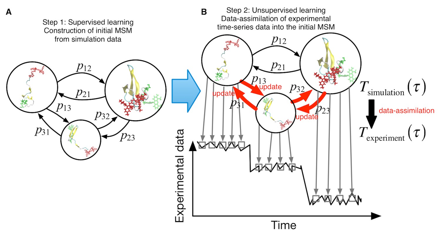
Schematic of proposed semi-supervised learning approach.
(A) Our proposed approach comprises two steps. As the first step, an initial Markov State Model is constructed only from simulation data by simply counting transitions between conformational states. (B) In the second step, transition probabilities (depicted by arrows) are updated through unsupervised learning from experimental time-series data.
Figure 1—figure supplement 1
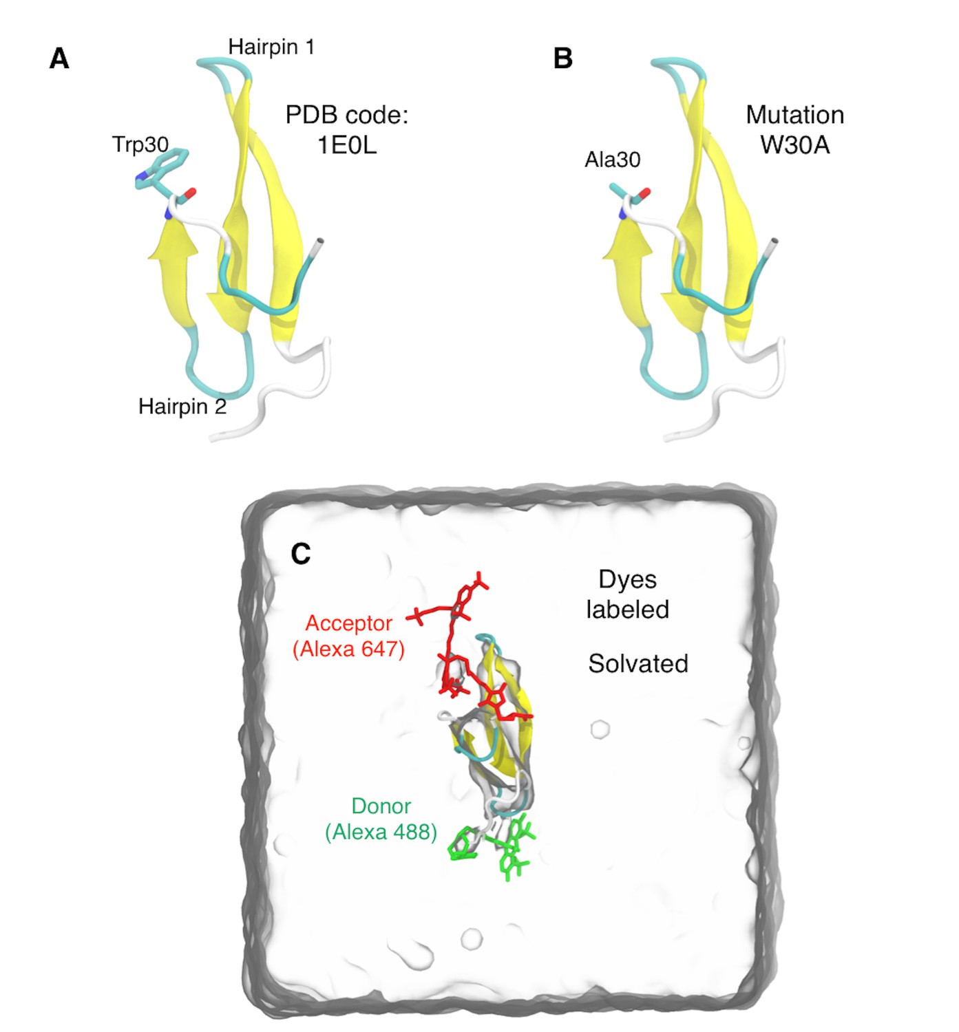
Dye-labeled WW domain and simulation box.
(A) NMR structure of FBP WW domain. (B) The same substitution mutation W30A as in experiments. (C) Donor (Alexa 488) and acceptor (Alexa 647) dyes attached to the WW domain. The protein is solvated with TIP3P water molecules under the periodic boundary condition.
Figure 2 with 9 supplements

Sampled conformations from simulations and Markov state models constructed in Q and expected FRET efficiency space.
(A) Scatter plot of sampled conformations from the aggregated trajectories. Representative structures from folded, compact unfolded, and elongated states are shown. Donor and acceptor dyes are colored green and red, respectively. (B) Cluster centers used for constructing the Markov state model are plotted with circles. (C) Initial Markov state model constructed from simulation data only. Node areas are proportional to the equilibrium populations, and edge line widths are proportional to the transition probabilities. (D) Data-assimilated Markov state model after unsupervised learning from smFRET photon-count sequences. Edges with transition probabilities of less than 0.01 are not shown for visual clarity.
Figure 2—figure supplement 1

Q of molecular dynamics simulation trajectories.
(A) Time-course behavior of the fraction of native contacts, Q, is shown for eleven 25.6 μs simulations (starting from unfolded states) and for six 10 μs and four 14 μs simulations (starting from the folded state). All simulations used the force-field of Amber ff99SB. (B) Time-course behavior with a modified Amber ff99SB force-field where the strength between water molecules and protein was scaled. Ten 7 μs simulations (starting from the unfolded states) are shown.
Figure 2—figure supplement 2
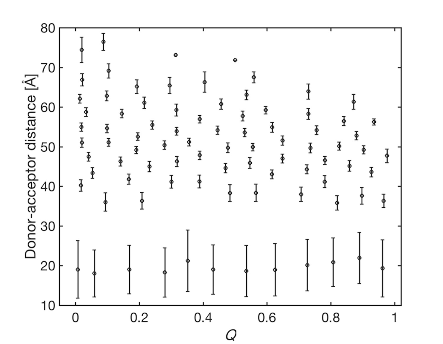
Donor-acceptor distances of the Markov states.
The Markov states are plotted in the space spanned by the donor-acceptor distance and Q. Circles represent mean values of two coordinates in the Markov states. The error bar represents the standard deviations of the donor-acceptor distances in the states.
Figure 2—figure supplement 3
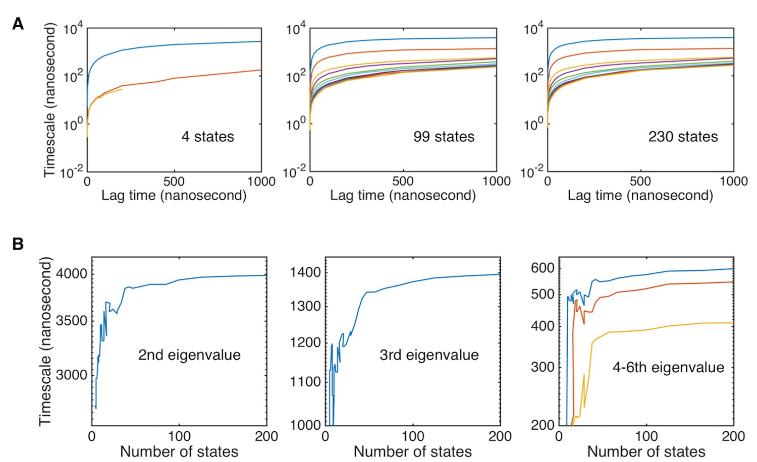
Implied timescales for various numbers of states.
(A) Implied timescales for Markov state models built with different numbers of states (4, 99, and 230 states). (B) Converged implied timescales as a function of the number of states. The timescales of the five slowest related to folding dynamics modes are shown.
Figure 2—figure supplement 4
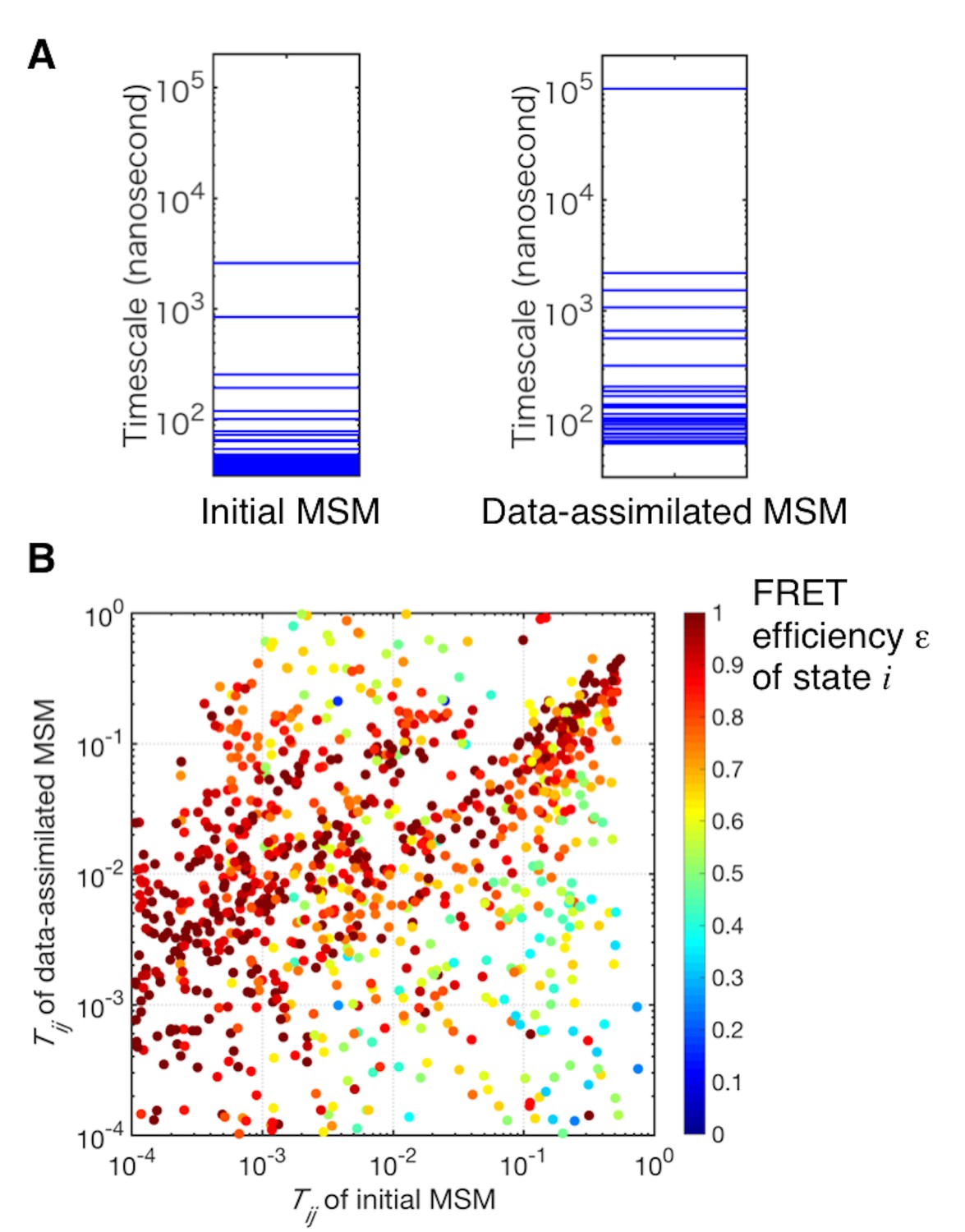
Comparison of the transition probabilities of the initial and the data-assimilated Markov state models.
(A) Implied time scales of the initial and the data-assimilated Markov state models. (B) Scatter plot of transition probabilities of the two models. The dots are colored by the FRET efficiencies of the states before transitions (i.e, state i of Tij).
Figure 2—figure supplement 5
Data-assimilated Markov state models using halves of the training data.
(A) Data-assimilated Markov state model obtained using one half set of the single-molecule FRET data. (B) Data-assimilated Markov state model using the other half set. Both models capture similar unfolded, folded, and intermediate states as populated states. Edges with transition probabilities of less than 0.01 are not shown for visual clarity.
Figure 2—figure supplement 6
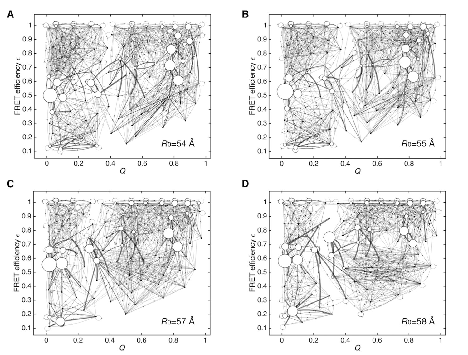
Dependency of data-assimilated Markov state models on the choice of Förster radius R0.
(A) Data-assimilated Markov state model after the convergence of the likelihood function by 10,000 iterations of unsupervised learning using a Förster radius of R0 = 54 Å. Edges with transition probabilities of less than 0.01 are not shown for visual clarity. (B) R0 = 55 Å. (C) R0 = 57 Å. (D) R0 = 58 Å.
Figure 2—figure supplement 7
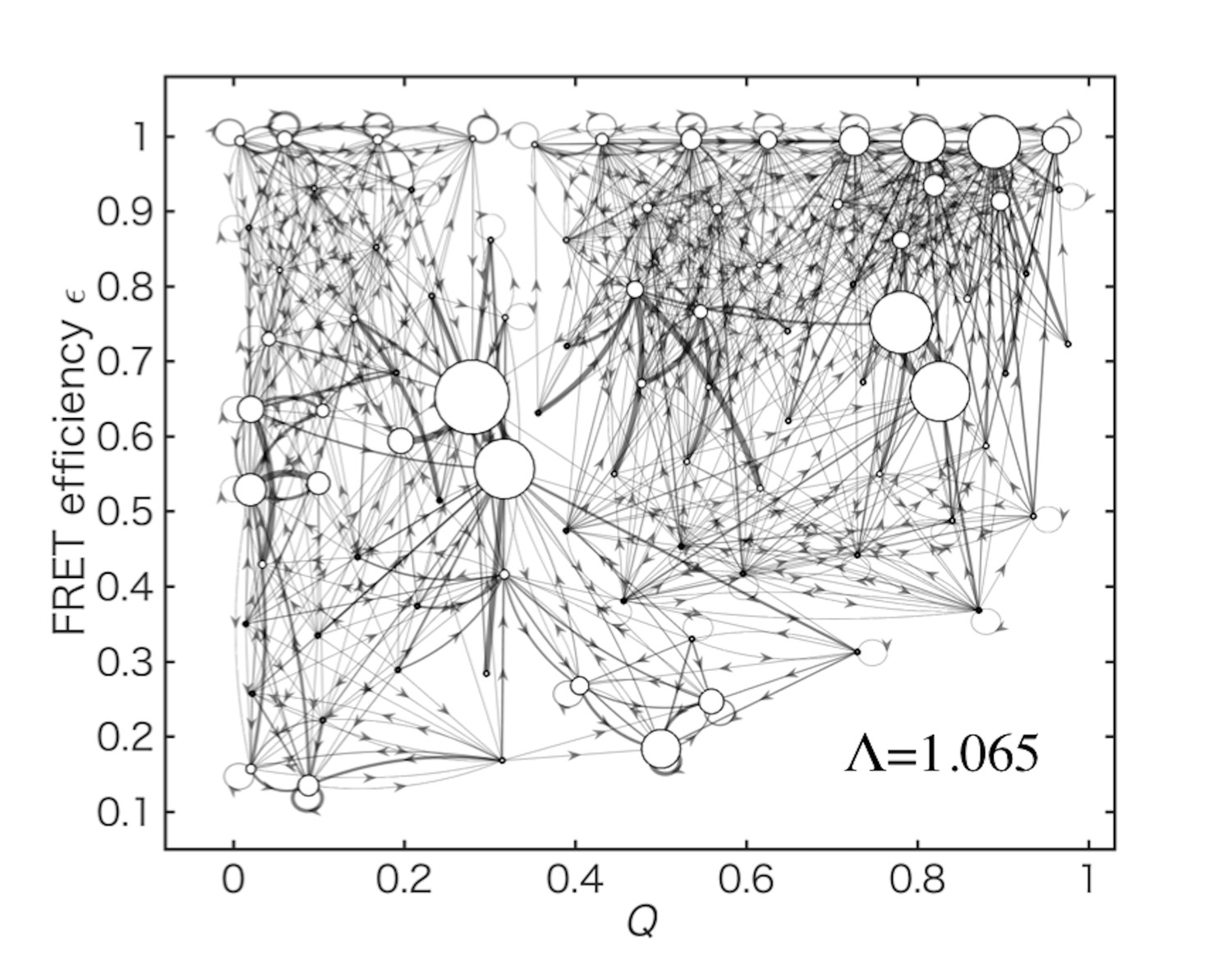
Data-assimilated Markov state obtained by considering the FRET efficiency outside the weak-excitation limit.
Data-assimilated Markov state model after the convergence of the likelihood function by 10,000 iterations. Here, a corrected definition of FRET efficiency, which is valid outside the weak-excitation limit (with a parameter ), was used for the calculation of the likelihood function.
Figure 2—figure supplement 8
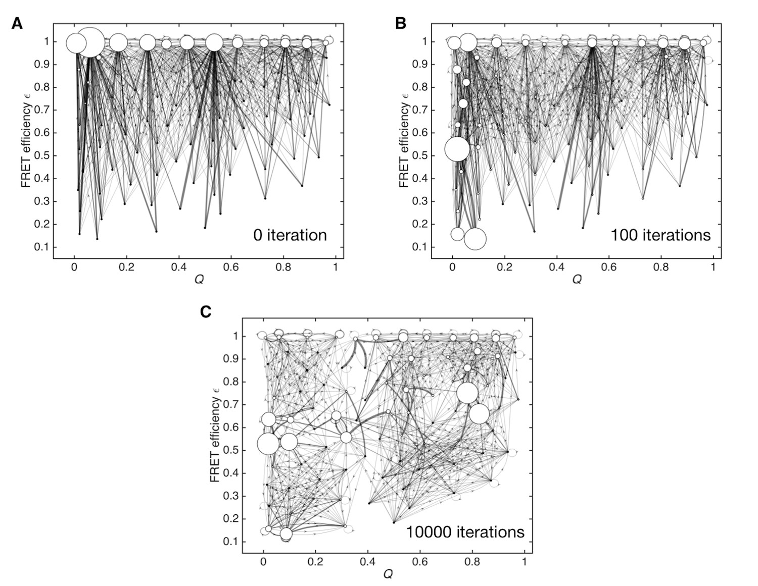
Optimization process for the initial Markov state model.
(A) Initial Markov state model constructed only from MD simulation data, used as an initial condition for the unsupervised learning. (B) Markov state model after 100 iterations of unsupervised learning. (C) Data-assimilated Markov state model after the convergence of the likelihood function by 10,000 iterations of unsupervised learning.
Figure 2—figure supplement 9
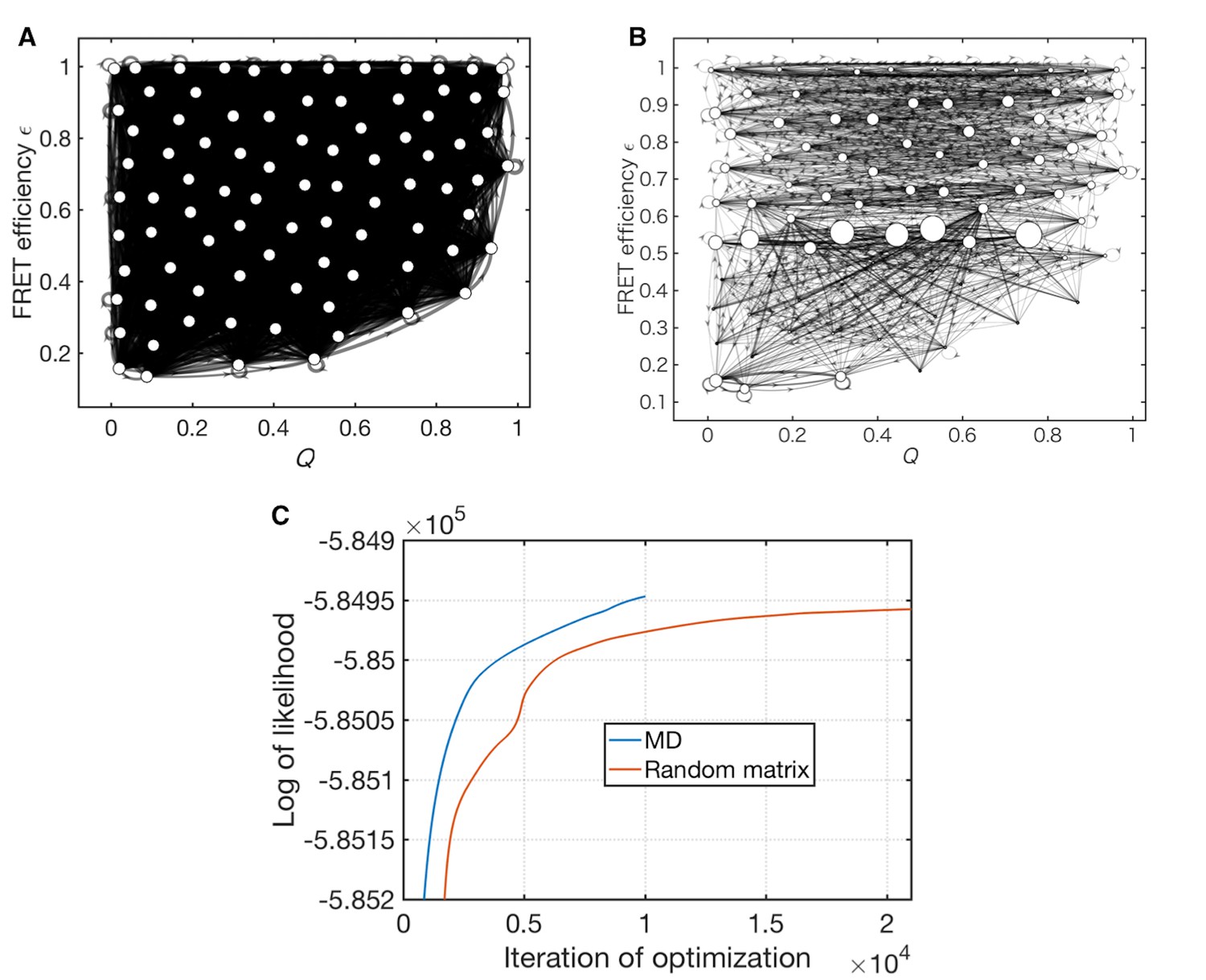
Optimization of a random matrix as the initial condition.
(A) Initial Markov state model constructed by assigning random values to the transition probabilities, used as an initial condition for the unsupervised learning. (B) Data-assimilated Markov state model after 21,331 iterations of unsupervised learning. (C) Convergence behavior of the likelihood functions. The blue line corresponds to the initial condition constructed from MD data. The red line indicates the initial condition given from a random matrix.
Figure 3 with 1 supplement
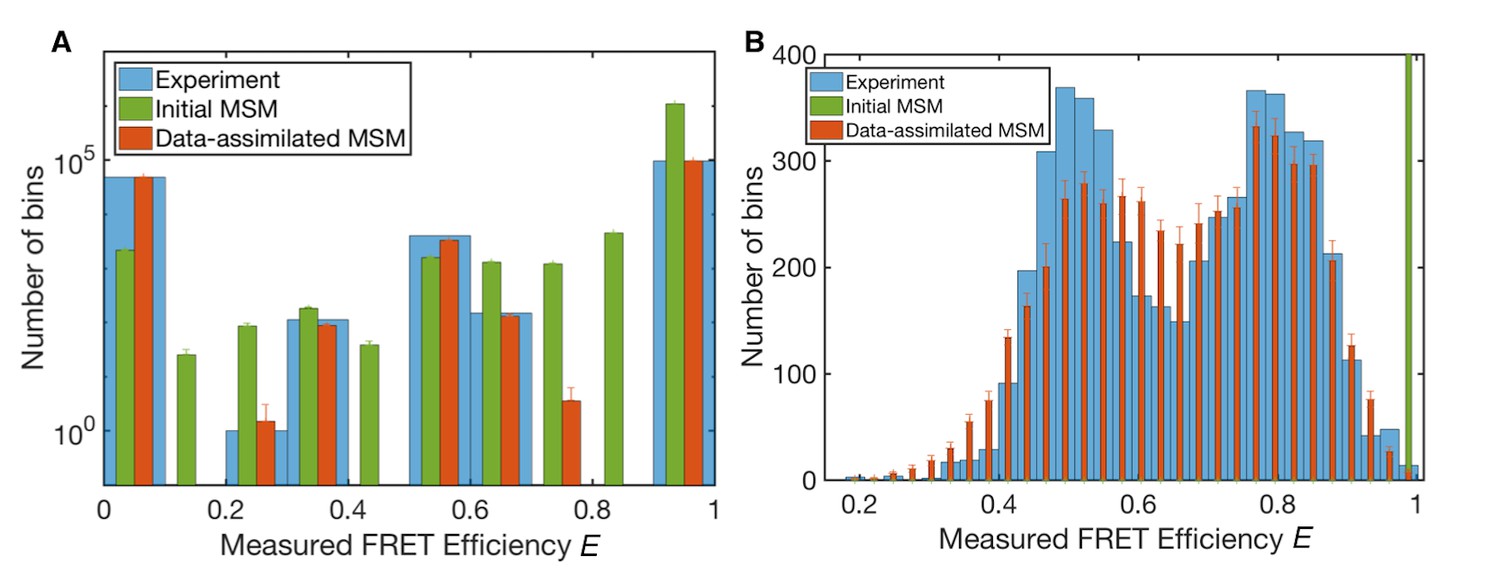
Measured FRET efficiency histograms.
(A) Measured FRET efficiency histograms calculated from donor and acceptor photons in the single-molecule FRET data with a time-window of 200 ns width, and those generated from initial and data-assimilated Markov state models. The measured FRET efficiency is defined as the ratio of the acceptor photon counts to the total number of photons (E = NA/(NA +ND)). Error bars indicate standard deviations in ten realizations of photon sequences for both models. (B) Measured FRET efficiency histograms calculated with a time-window of 50 μs.
Figure 3—figure supplement 1
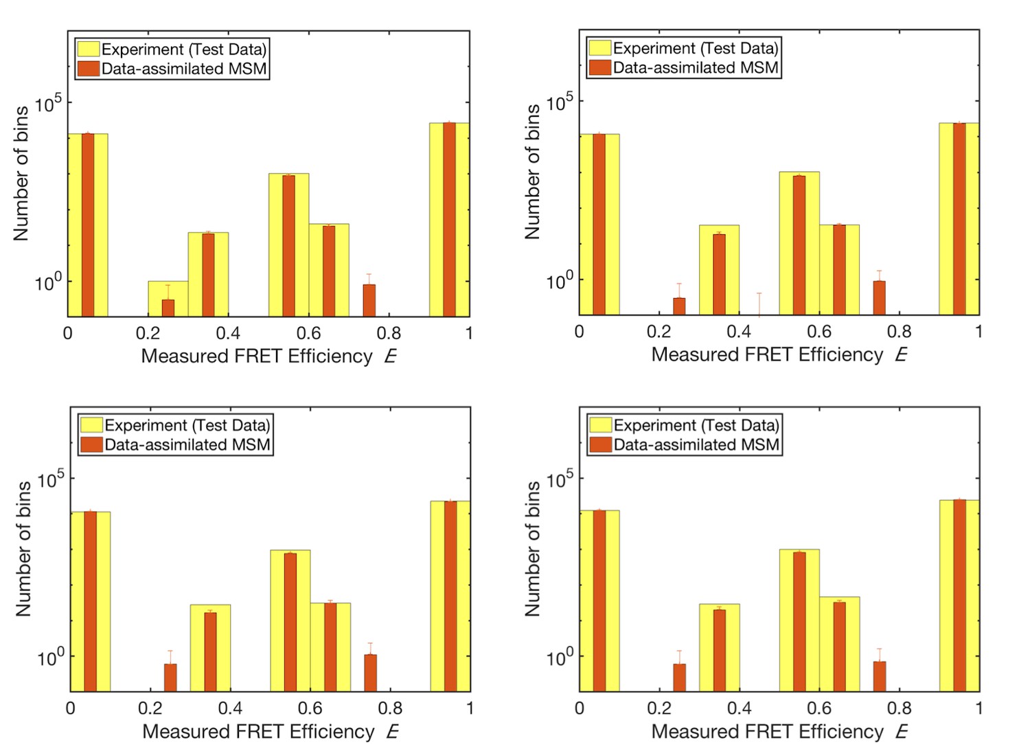
k-fold cross validation test.
The results of a k-fold cross validation test (with k = 4). Comparison of the histograms of measured FRET efficiency calculated from the test data (not used for unsupervised learning) and the prediction by stochastic simulation with the trained model (i.e., the data-assimilated Markov state model).
Figure 4 with 1 supplement
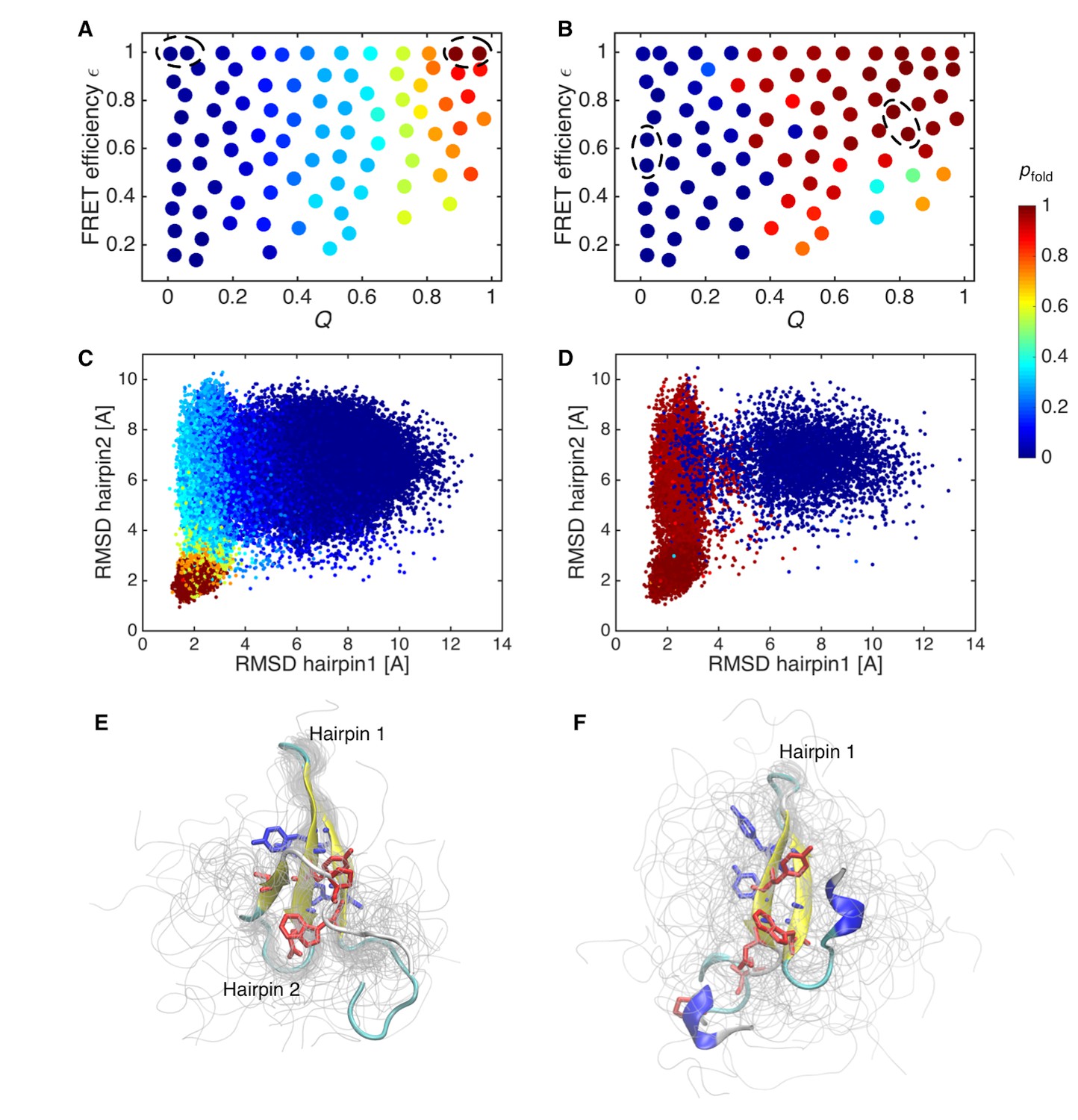
Probability of folding, pfold, and transition state ensemble.
(A) Probabilities of folding, pfold, mapped onto the states of initial Markov state model. (B) pfold for data-assimilated Markov state model. The unfolded and folded states used for the calculation (source and sink in the context of the transition path theory, respectively) are indicated by circles. (C) Trajectory snapshots in the the RMSDs of hairpins 1 and 2 from their native structures are colored by pfold for the initial Markov state model. (D) Trajectory snapshots of the data-assimilated Markov state model. (E) Structures of the transition state ensemble in the initial Markov state model which correspond to pfold = 0.4–0.6. (F) The transition state ensemble in the data-assimilated Markov state model. Two hydrophobic cores that project below and above the plane of the sheet, core 1 (Trp8, Tyr20, Asn22, Thr29, Pro33, shown in red) and core 2 (Thr9, Tyr11, Tyr 19, Tyr21, shown in blue) are represented by sticks.
Figure 4—figure supplement 1
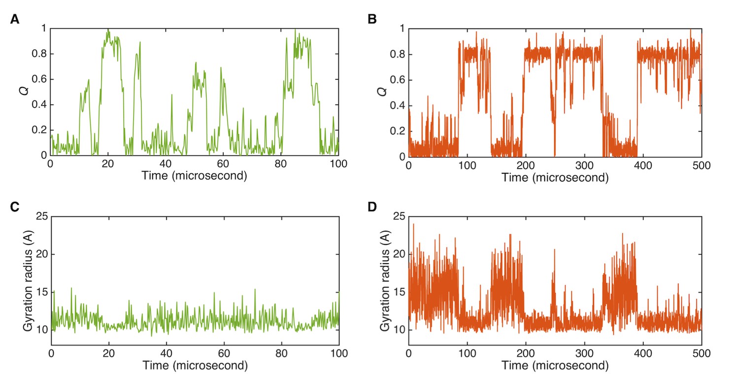
Dynamics of initial and data-assimilated Markov state models.
(A) Time-course plot of the fraction of native contacts, Q, for the initial Markov state model. (B) Q of data-assimilated Markov state model. (C) Time-course plot of gyration radius for initial Markov state model. (D) Gyration radius of the data-assimilated Markov state model.
Figure 5
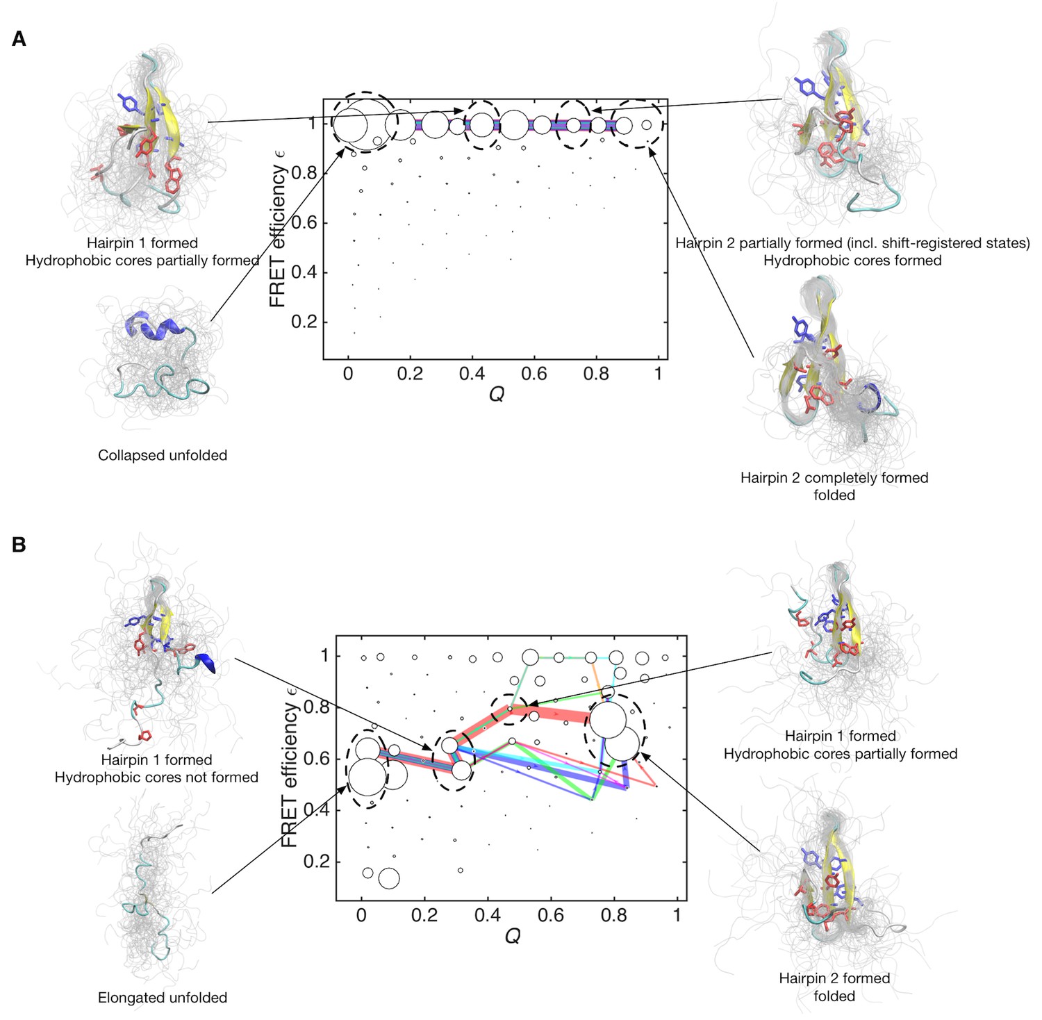
Folding pathways for initial and data-assimilated Markov state models.
(A) Folding flux of the initial Markov state model was decomposed into individual folding pathways. Folding pathways with largest fluxes contributing 50% of the total flux are superimposed in different colors. In this case, all of the pathways are located at expected FRET efficiency ε ~ 1 with different step size in the Q axis. Line widths are proportional to fluxes. Structures of representative states are shown. Two hydrophobic cores that project below and above the plane of the sheet, core 1 (Trp8, Tyr20, Asn22, Thr29 and Pro33, shown in red) and core 2 (Thr9, Tyr11, Tyr 19 and Tyr21, shown in blue) are represented by sticks. (B) Folding pathways with largest fluxes contributing 50% of the total flux are shown for the data-assimilated Markov state model.
Additional files
-
Transparent reporting form
- https://doi.org/10.7554/eLife.32668.019
Download links
A two-part list of links to download the article, or parts of the article, in various formats.
Downloads (link to download the article as PDF)
Open citations (links to open the citations from this article in various online reference manager services)
Cite this article (links to download the citations from this article in formats compatible with various reference manager tools)
Linking time-series of single-molecule experiments with molecular dynamics simulations by machine learning
eLife 7:e32668.
https://doi.org/10.7554/eLife.32668


