Robust model-based analysis of single-particle tracking experiments with Spot-On
- University of California, Berkeley, United States
- Howard Hughes Medical Institute, United States
- Institut Pasteur, France
- Sorbonne Universités, France
- Janelia Research Campus, Howard Hughes Medical Institute, United States
Figures
Figure 1

Bias in single-particle tracking (SPT) experiments and analysis methods.
(A) ‘Motion-blur’ bias. Constant excitation during acquisition of a frame will cause a fast-moving particle to spread out its emission photons over many pixels and thus appear as a motion-blur, which make detection much less likely with common PSF-fitting algorithms. In contrast, a slow-moving or immobile particle will appear as a well-shaped PSF and thus readily be detected. (B) Tracking ambiguities. Tracking at high particle densities prevents unambiguous connection of particles between frames and tracking errors will cause displacements to be misidentified. (C) Defocalization bias. During 2D-SPT, fast-moving particles will rapidly move out-of-focus resulting in short trajectories, whereas immobile particles will remain in-focus until they photobleach and thus exhibit very long trajectories. This results in a bias toward slow-moving particles, which must be corrected for. (D) Analysis method. Any analysis method should ideally avoid introducing biases and accurately correct for known biases in the estimation of subpopulation parameters such as DFREE, FBOUND, DBOUND.
Figure 2
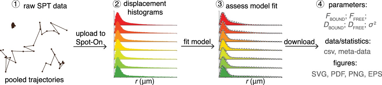
Overview of Spot-On interface.
To use Spot-On, a user uploads raw SPT data in the form of pooled SPT trajectories to the Spot-On web-interface. Spot-On then calculates displacement histograms. The user inputs relevant experimental descriptors and chooses a model to fit. After model-fitting, the user can then download model-inferred parameters, meta-data and download publication-quality figures.
Figure 3 with 12 supplements
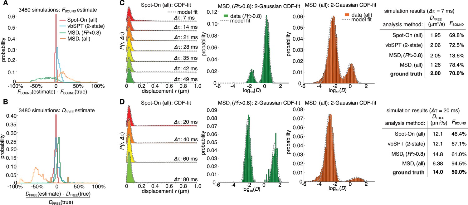
Validation of Spot-On using simulations and comparisons to other methods.
(A–B) Simulation results. Experimentally realistic SPT data was simulated inside a spherical mammalian nucleus with a radius of 4 μm subject to highly-inclined and laminated optical sheet illumination (Tokunaga et al., 2008) (HiLo) of thickness 4 μm illuminating the center of the nucleus. The axial detection window was 700 nm with Gaussian edges and particles were subject to a 25 nm localization error in all three dimensions. Photobleaching corresponded to a mean trajectory length of 4 frames inside the HiLo sheet and 40 outside. 3480 experiments were simulated with parameters of DFREE=[0.5;14.5] in steps of 0.5 μm2/s and FBOUND=[0;95% in steps of 5% and the frame rate correspond to Δτ=[1,4,7,10,13,20] ms. Each experiment was then fitted using Spot-On, using vbSPT (maximum of 2 states allowed) (Persson et al., 2013), MSDi using all trajectories of at least five frames (MSDi (all)) or MSDi using all trajectories of at least five frames where the MSD-curvefit showed at least R2 >0.8 (MSDi (R2 >0.8)). (A) shows the distribution of absolute errors in the FBOUND–estimate and (B) shows the distribution of relative errors in the DFREE–estimate. (C) Single simulation example with DFREE = 2.0 µm2/s; FBOUND = 70%; 7 ms per frame. The table on the right uses numbers from CDF-fitting, but for simplicity the fits to the histograms (PDF) are shown in the three plots. (D) Single simulation example with DFREE = 14.0 µm2/s; FBOUND = 50%; 20 ms per frame. Full details on how SPT data was simulated and analyzed with the different methods is given in Appendix 1.
Figure 3—figure supplement 1
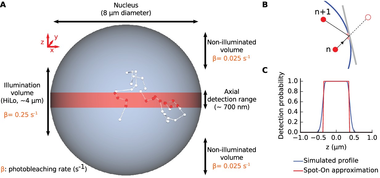
Overview of SPT simulations.
(A) Trajectories were simulated in a confined volume: a ‘nucleus’ of 8 µm diameter, in which molecules are photoactivated at random and photobleach when located within the HiLo volume (a ~4 µm thick slice). Molecules are detected when they are within the axial detection range of the objective (~700 nm). (B) confinement within the nucleus was achieved by specular reflections against the nuclear envelope: a particle bumping on the nuclear envelope is ballistically reflected inside. (C) axial detection profile used for the simulation (blue): flat-top Gaussian with 600 nm plateau and 100 nm FWHM for the Gaussian edges. (red): approximated axial detection profile assumed by Spot-On (step function with 700 nm width).
Figure 3—figure supplement 2
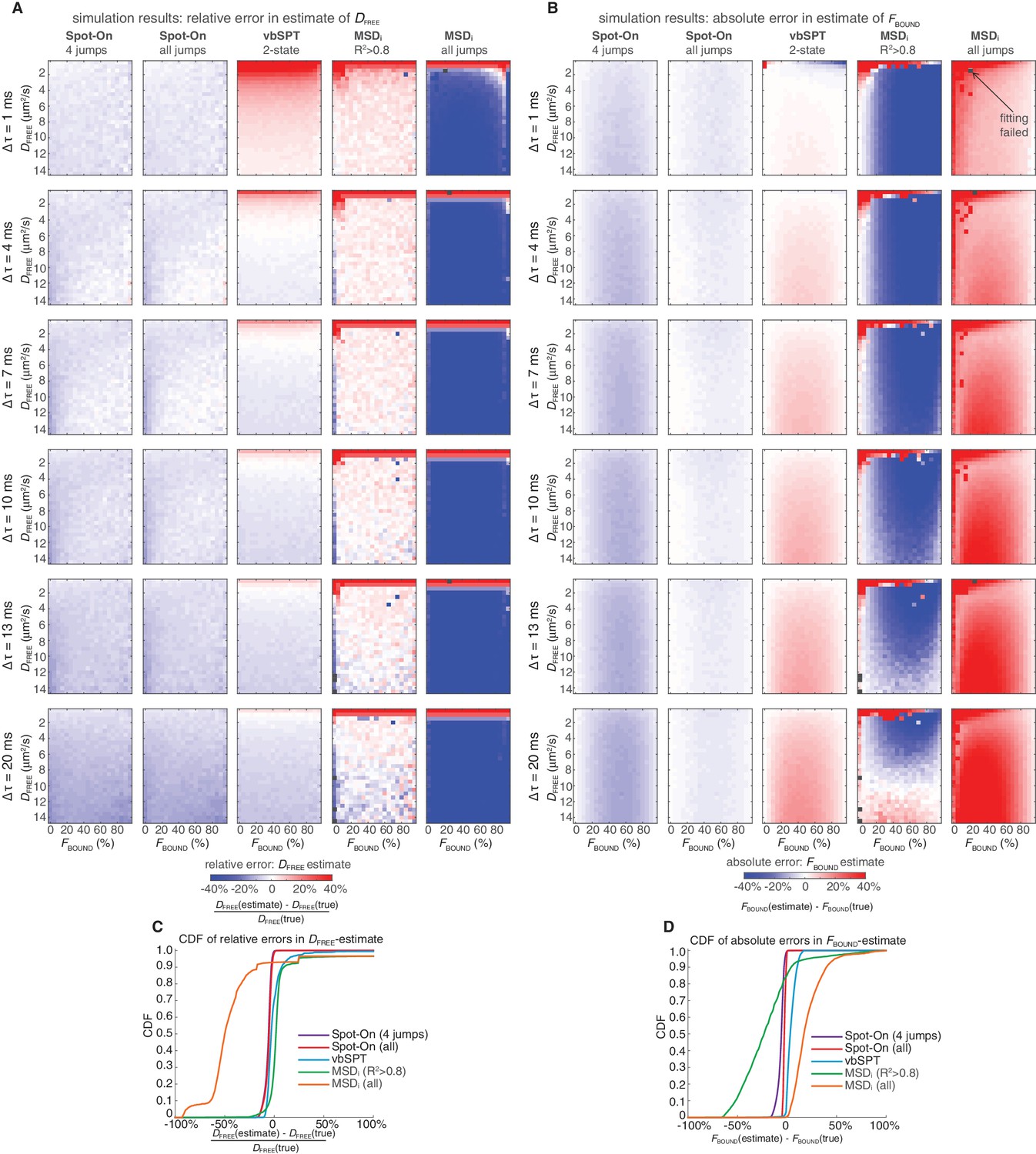
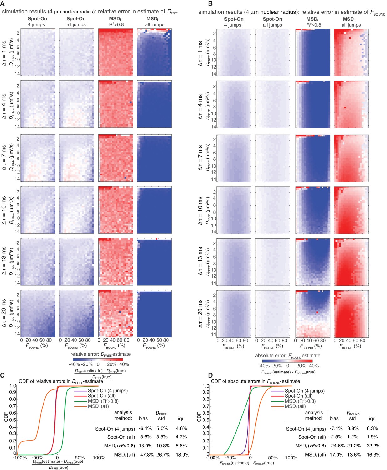
Comparison of Spot-On, vbSPT and MSDi estimates of DFREE and FBOUND to ground-truth simulation results inside a 4 µm radius nucleus.
Heatmaps showing errors in Spot-On, vbSPT and MSDi estimates of DFREE (A) and FBOUND (B). To comprehensively test Spot-On and alternative analysis methods such as vbSPT and MSDi (Appendix 1), we analyzed 3480 simulations using these methods. The simulations are available for download (see ‘Data availability’) and the code used for the simulations is available at GitLab (https://gitlab.com/tjian-darzacq-lab/simSPT). Briefly, experimentally realistic SPT experiments were simulated assuming 2-state (free or bound) Brownian motion inside a nucleus of 4 µm radius illuminated using HiLo illumination (assuming a HiLo beam width of 4 µm), with an axial detection range of ~700 nm, centered at the middle of the HiLo beam. In (A), the heatmaps show the relative error and in (B) the heatmaps show the absolute error. In a few rare cases (marked by black squares), the MSDi-method failed such that no estimate was possible. Cumulative distribution function (CDF) plots of the relative error in the DFREE–estimate (C) and the absolute error in the FBOUND–estimate (D).
Figure 3—figure supplement 3
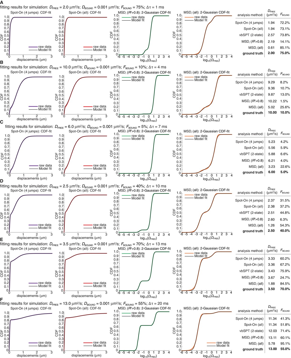
Representative fits for Spot-On, vbSPT and MSDi to ground-truth simulations.
(A) fits to simulation where DFREE = 2.0 µm2/s; FBOUND = 75%; 1 ms per frame. First column: Spot-On CDF-fit with JumpsToConsider = 4; only CDF-fit at 3Δt is shown. Second column: Spot-On CDF-fit using all jumps; only CDF-fit at 3Δt is shown. Third column: MSDi-CDF-fit to log10(DFREE) considering only trajectories of at least five frames, where the MSD-fit to a single trajectory was good (R2 >0.8). Fourth column: MSDi-CDF-fit to log10(DFREE) considering only trajectories of at least five frames, but without a MSD-fit threshold. Fifth column: table comparing all the four methods as well as vbSPT (2-state) estimates of DFREE and FBOUND to the ground truth used for the simulations. (B) fits to simulation where DFREE = 10.0 µm2/s; FBOUND = 10%; 4 ms per frame. Each column is described in (A). (C) fits to simulation where DFREE = 6.0 µm2/s; FBOUND = 5%; 7 ms per frame. Each column is described in (A). (D) fits to simulation where DFREE = 2.5 µm2/s; FBOUND = 40%; 10 ms per frame. Each column is described in (A). (E) fits to simulation where DFREE = 3.5 µm2/s; FBOUND = 70%; 13 ms per frame. Each column is described in (A). (F) fits to simulation where DFREE = 13.0 µm2/s; FBOUND = 55%; 20 ms per frame. Each column is described in (A).
Figure 3—figure supplement 4
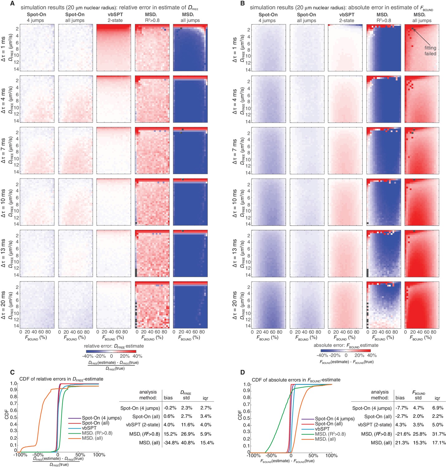
Comparison of Spot-On, vbSPT and MSDi estimates of DFREE and FBOUND to ground-truth simulations inside a 20 µm radius nucleus.
Heatmaps showing errors in Spot-On, vbSPT and MSDi estimates of DFREE (A) and FBOUND (B). To comprehensively test Spot-On and alternative analysis methods such as vbSPT (Persson et al., 2013) and MSDi (Appendix 1), we analyzed 3480 simulations (described in Figure 3—figure supplement 2) using these methods. In (A), the heatmaps show the relative error and in (B) the heatmaps show the absolute error. In a few rare cases (marked by black squares), the MSDi-method failed such that no estimate was possible. Note that whereas Spot-On would always underestimate DFREE inside a small 4 µm radius nucleus, when the confinement is largely relaxed by considering a 20 µm radius nucleus, Spot-On now shows essentially no bias in its DFREE–estimate. Cumulative distribution function (CDF) plots and summary tables of the relative error in the DFREE–estimate (C) and the absolute error in the FBOUND–estimate (D). Bias refers to the mean error, ‘std’ is the standard deviation and ‘iqr’ is the inter-quartile range (difference between the 75th and 25th percentile).
Figure 3—figure supplement 5
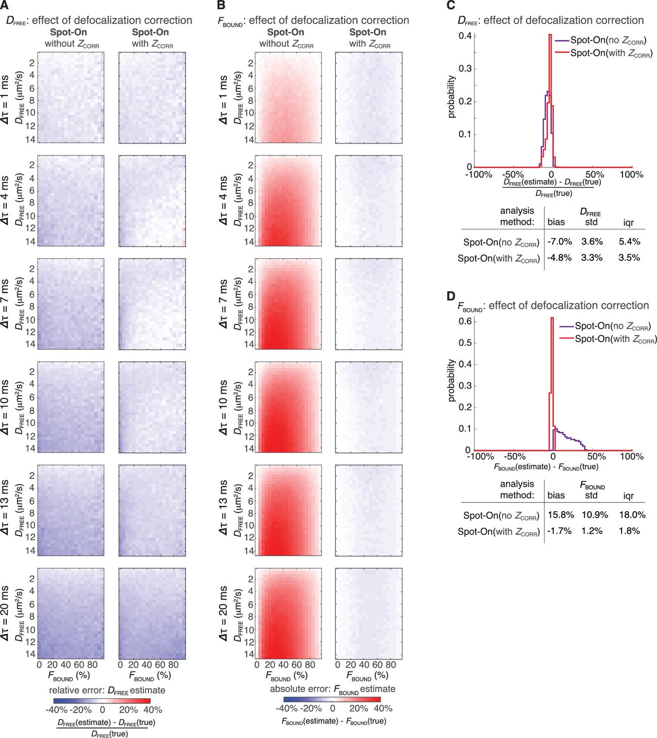
Effect of defocalization bias correction.
In order to determine how important correcting for defocalization bias is, we analyzed the 3480 simulations using Spot-On (all) and exactly the same parameters as in Figure 3A–B except without the defocalization bias correction, ZCORR. Heatmaps show errors in Spot-On (all; with ZCORR) and Spot-On (all; without ZCORR) estimates of DFREE (A) and FBOUND (B). Histogram plots and summary statistics tables of the relative error in the DFREE–estimate (C) and the absolute error in the FBOUND–estimate (D). As can be seen, correcting for defocalization bias slightly improves the DFREE–estimate, but is essential for an accurate FBOUND–estimate. As expected, the longer the lag time, the more important it is to correct for defocalization bias.
Figure 3—figure supplement 6

Evaluation of the 3-states model.
Trajectories were simulated using simSPT for a 3-state model. Three representative fractions were picked and for each of them, one state was always bound (DBOUND = 0.001 µm²/s) and the two other states were varied (0.5–11 µm²/s), together with the framerate (1–20 ms), yielding 720 conditions. The simulations were then either fitted with Spot-On or vbSPT constrained to infer up to three states. (A) Distribution of the error of five of the inferred parameters (DSLOW, DFAST, FBOUND, FSLOW, FFAST) with respect to ground truth for Spot-On (red) and vbSPT (blue). The top row shows the distribution and the bottom row the cumulative distribution. (B-G) For each of the three fractions configurations (25/25/50, 25/50/25, 50/25/25%, for B-C, D-E, F-G, respectively), detailed error on five inferred parameters (columns) for different frame rates (rows) and various DSLOW and DFAST (rows and columns of the matrix, respectively). (H) summary table showing the mean error (bias) and standard deviation over all the simulations.
Figure 3—figure supplement 7
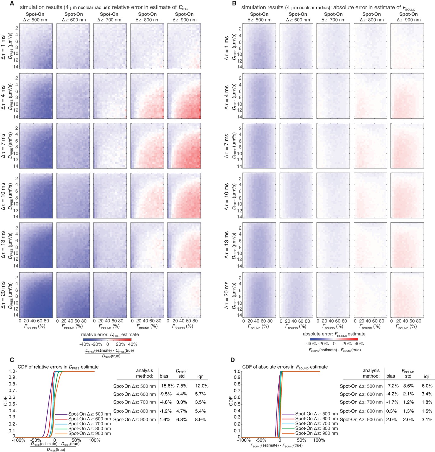
Sensitivity of Spot-On to the axial detection range estimate.
Heatmaps showing errors in Spot-On estimates of DFREE (A) and FBOUND (B) as a function of the axial detection range, Δz. The simulations were as described in Figure 3—figure supplement 2. Rather than an unrealistic step function, the simulated axial detection range has Gaussian edges with FWHM of 700 nm. Spot-On analysis parameters were exactly as for Spot-On (all) in Figure 3—figure supplement 2, except the axial detection range, Δz, was set to either 500 nm, 600 nm, 700 nm, 800 nm or 900 nm. As can be seen, Spot-On is only mildly sensitive to small errors (~100 nm) in the axial detection range estimate. In (A), the heatmaps show the relative error and in (B) the heatmaps show the absolute error. Cumulative distribution function (CDF) plots of the relative error in the DFREE–estimate (C) and the absolute error in the FBOUND–estimate (D) as well as summary tables.
Figure 3—figure supplement 8
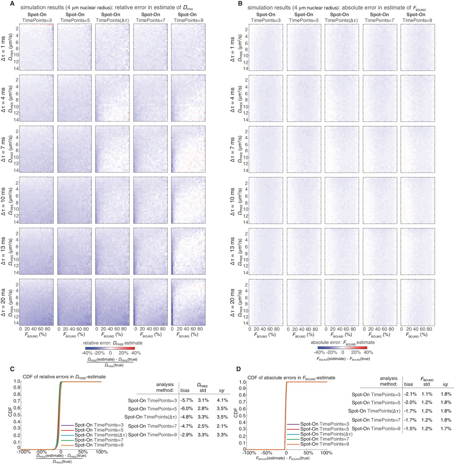
Sensitivity of Spot-On to the number of time points considered.
Heatmaps showing errors in Spot-On estimates of DFREE (A) and FBOUND (B) as a function of the number of time points considered. Note that if TimePoints = n, the number of displacements that will be considered goes from one to (n-1). The simulations were as described in Figure 3—figure supplement 2. Spot-On analysis parameters were exactly as for Spot-On (all) in Figure 3—figure supplement 2, except the TimePoints parameter was set to either 3, 5, 7, 9 or dependent on the frame rate (TimePoints(Δτ)) as in Figure 3—figure supplement 2 and described in Appendix 1. As can be seen, Spot-On is not very sensitive to how many TimePoints were considered. However, when working with small datasets of experimental data, if there is not enough data at higher TimePoints values, noise can make the estimates unreliable. In (A), the heatmaps show the relative error and in (B) the heatmaps show the absolute error. Cumulative distribution function (CDF) plots of the relative error in the DFREE–estimate (C) and the absolute error in the FBOUND–estimate (D) as well as summary tables.
Figure 3—figure supplement 9
Comparison of Spot-On and MSDi estimates of DFREE and FBOUND to ground-truth simulation results inside a 4 µm radius nucleus using PDF-fitting.
Heatmaps showing errors in Spot-On and MSDi estimates of DFREE (A) and FBOUND (B). The analysis was performed identically to Figure 3—figure supplement 2 except PDF-fitting was performed instead of CDF-fitting. In (A), the heatmaps show the relative error and in (B) the heatmaps show the absolute error. Cumulative distribution function (CDF) plots of the relative error in the DFREE–estimate (C) and the absolute error in the FBOUND–estimate (D).
Figure 3—figure supplement 10
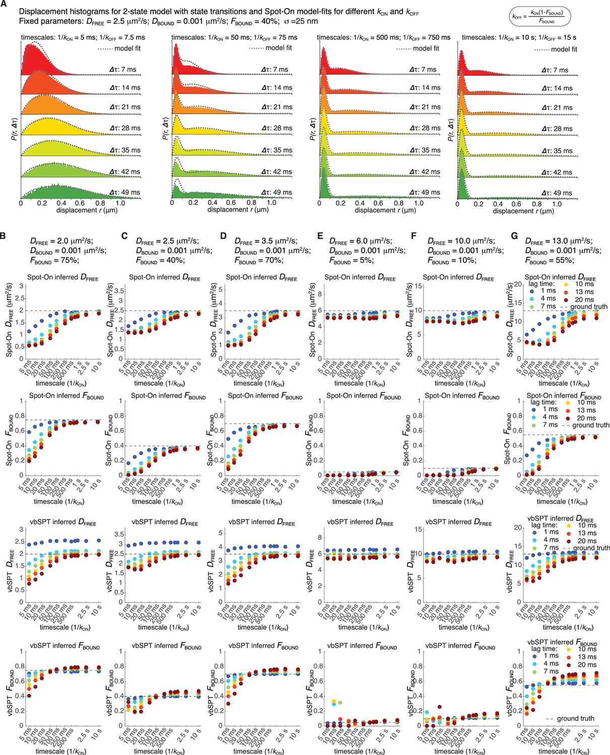
Sensitivity of Spot-On to state changes and comparison with vbSPT.
For six different representative conditions (combinations of DFREE and FBOUND; DBOUND = 0.001 µm²/s; σ = 25 nm), we simulated 100,000 trajectories using simSPT and included state transitions (e.g. transition from bound to free) considering six different lag time (1, 4, 7, 10, 13 and 20 ms) and kON values from 0.1 s−1 to 200 s−1 yielding a total of 396 simulations. The data were analyzed using Spot-On (all) as in Figure 3A–B. (A) For one example parameter set, (A) shows how the histogram of displacements and the goodness of the Spot-On model-fit changes as state transition go from more frequent than the frame rate (left) to very infrequent (right). (B-G), First row: shows sensitivity of the Spot-On estimate of DFREE to the timescale of state transitions. The values of DFREE and FBOUND are shown above the plot. (B-G), Second row: shows sensitivity of the Spot-On estimate of FBOUND to the timescale of state transitions. (B-G), Third row: shows sensitivity of the vbSPT estimate of DFREE to the timescale of state transitions. The values of DFREE and FBOUND are shown above the top plot. (B-G), Fourth row: shows sensitivity of the vbSPT estimate of FBOUND to the timescale of state transitions. As expected, since Spot-On ignores state transitions, the inference breaks down when the timescale of state transitions becomes comparable to the frame rate. Perhaps surprisingly, vbSPT also breaks down when state transitions are frequent despite explicitly modeling this in the Hidden Markov Model. Also as expected, a faster frame rate (e.g. 1 ms in dark blue) can support a faster state transition rate. Nevertheless, as long as the timescale of transitions is at least a few hundred milliseconds, Spot-On is not strongly affected. For comparison, the residence time of most mammalian transcription factors is tens of seconds.
Figure 3—figure supplement 11

Robustness of localization error estimates from Spot-On.
For six different representative conditions (combinations of DFREE and FBOUND; DBOUND = 0.001 µm²/s), we simulated 100,000 trajectories using simSPT keeping everything as in Figure 3A–B except varying the localization error (σ) from 10 nm to 75 nm in 5 nm steps and considering six different lag time (1, 4, 7, 10, 13 and 20 ms) yielding a total of 504 simulations. The data were analyzed using Spot-On (all) as in Figure 3A–B except here the localization error was inferred from the fitting. (A-F), top row: show how well the Spot-On inferred the localization error vs. the simulated localization error and the lag times are color coded. The values of DFREE and FBOUND are shown above the plot. (A-F), bottom row: histograms showing the distribution of errors in the localization error estimate across all lag time and σ-values for a given combinations of DFREE and FBOUND. (G) Table showing summary statistics from the fitting in (A-F). We note that in all cases where the bound fraction is significant (>10%), Spot-On robustly infers the localization error (mean error below 1.5 nm), whereas in cases where the bound fraction is small (10% or below), the localization error estimate becomes less robust (mean error ~3–6 nm). This is because Spot-On can most reliably use how the displacement distribution of the bound fraction changes over time to infer the localization error (see also Materials and Methods).
Figure 3—figure supplement 12
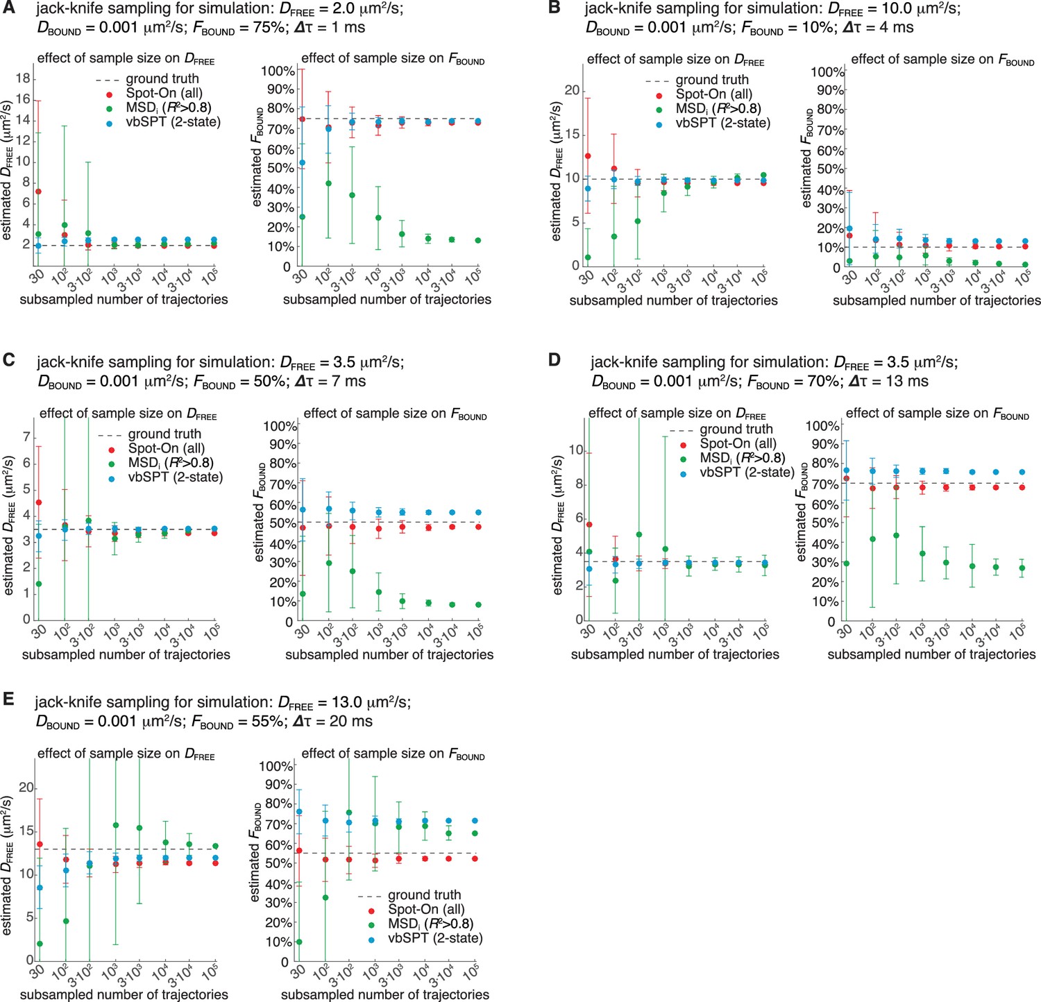
Sensitivity of Spot-On, vbSPT and MSDi (R2 >0.8) to sample size.
(A) Jack-knife data sampling for simulation with DFREE = 2.0 µm2/s; FBOUND = 75%; 1 ms per frame. Simulated data (inside a 4 µm radius nucleus) was used. 100,000 trajectories with a mean photo-bleaching life-time of 4 frames were simulated and then subsampled 50 times without replacement. Sample sizes of either 30, 100, 300, 1,000, 3,000, 10,000, 30,000 or 100,000 trajectories were then fit using Spot-On (all), vbSPT (2-state model) or MSDi (R2 >0.8) as described in the analysis of simulations section. Error bars show standard deviation among the 50 sub-samplings. We note that occasionally, no more than ~5% of the time in the case of 30 trajectories, not a single trajectory of sufficient length for Spot-On or MSDi (R2 >0.8) was found. In these cases, we re-sampled to obtain at least one trajectory of sufficient length. Left plot shows effect of sample size on the DFREE–estimate. Right plot shows effect of sample size on the FBOUND–estimate. The dashed line shows the ground truth used to simulate the SPT data. (A) Jack-knife data sampling for simulation with DFREE = 10.0 µm2/s; FBOUND = 10%; 4 ms per frame. Everything else is as described in (A). (C) Jack-knife data sampling for simulation with DFREE = 3.5 µm2/s; FBOUND = 50%; 7 ms per frame. Everything else is as described in (A). (D) Jack-knife data sampling for simulation with DFREE = 3.5 µm2/s; FBOUND = 70%; 13 ms per frame. Everything else is as described in (A). (E) Jack-knife data sampling for simulation with DFREE = 13.0 µm2/s; FBOUND = 55%; 20 ms per frame. Everything else is as described in (A).
Figure 4 with 3 supplements
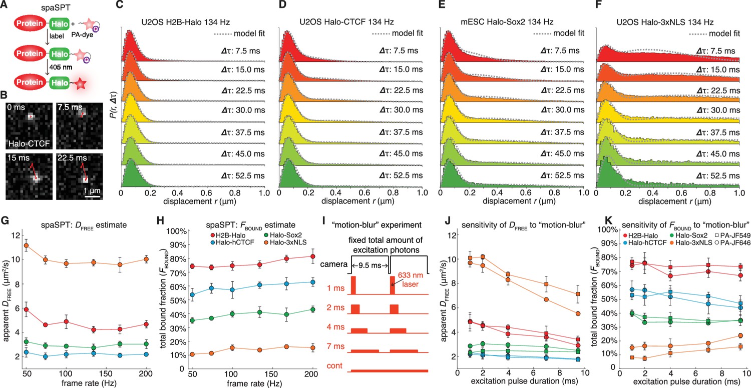
Overview of spaSPT and experimental results.
(A) spaSPT. HaloTag-labeling with UV (405 nm) photo-activatable dyes enable spaSPT. spaSPT minimizes tracking errors through photo-activation which maintains low densities. (B) Example data. Raw spaSPT images for Halo-CTCF tracked in human U2OS cells at 134 Hz (1 ms stroboscopic 633 nm excitation of JF646). (C–F) Histograms of displacements for multiple Δτ of histone H2B-Halo in U2OS cells (C), Halo-CTCF in U2OS cells (d), Halo-Sox2 in mES cells (E) and Halo-3xNLS in U2OS cells (F). (G–H) Effect of frame-rate on DFREE and FBOUND. spaSPT was performed at 200 Hz, 167 Hz, 134 Hz, 100 Hz, 74 Hz and 50 Hz using the 4 cell lines and the data fit using Spot-On and a 2-state model. Each experiment on each cell line was performed in four replicates on different days and ~5 cells imaged each day. (I) Motion-blur experiment. To investigate the effect of ‘motion-blurring’, the total number of excitation photons was kept constant, but delivered during pulses of duration 1, 2, 4, 7 ms or continuous (cont) illumination. (J–K) Effect of motion-blurring on DFREE and FBOUND. spaSPT data was recorded at 100 Hz and 2-state model-fitting performed with Spot-On. The inferred DFREE (J) and FBOUND (K) were plotted as a function of excitation pulse duration. Each experiment on each cell line was performed in four replicates on different days and ~5 cells imaged each day. Error bars show standard deviation between replicates.
Figure 4—figure supplement 1
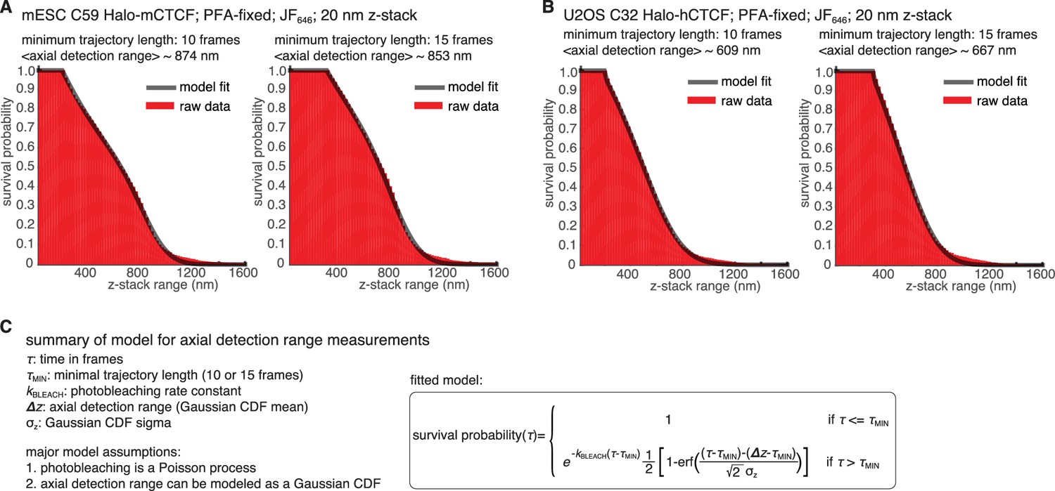
Experimental measurement of axial detection range.
To determine the axial detection range, mESC C59 Halo-mCTCF (Hansen et al., 2017) and U2OS C32 Halo-hCTCF (Hansen et al., 2017) cells were grown overnight on plasma-cleaned coverslips, labelled with 250 pM JF646, fixed in 4% PFA in PBS for 20 min, washed with PBS and then imaged in PBS with 0.01% (w/v) NaN3. We imaged the fixed cells using longer exposure times and very low 633 nm laser intensity to minimize photo-bleaching and collected a 6 µm z-stack spanning most of a nucleus using 20 nm steps. We optimized the imaging conditions to give near identical signal-to-noise to our spaSPT conditions and the data shown is merged data from at least 15 different cells for each cell line. We then localized and ‘tracked’ molecules to determine the experimental axial detection range. (A-B) show empirical survival probability distribution for PFA-fixed mESC C59 JF646Halo-mCTCF (A) and PFA-fixed U2OS C32 JF646Halo-hCTCF (B). A minimal threshold, τMIN, was set to filter out noise and the left plot shows τMIN=10 frames and the right plot τMIN=15 frames. The raw data is shown in red and a model-fit is overlaid. The estimated axial detection range is also shown. We note that the numbers depend somewhat on the threshold set and differ a bit between U2OS and mES cells. As an approximate average, we used 700 nm here. Importantly, we note that Spot-On is relatively robust to the axial detection range estimate and that changing it by 100 nm only marginally changes the results (Figure 3—figure supplement 7) (C) summary of the model that was fit to the data and the key model parameters. The model assumes that photo-bleaching is a Poisson process and that the axial detection range can be modeled as a Gaussian CDF. Raw data used to plot (A-B) and code for reproducing this figure and the model-fitting is available on GitLab: https://gitlab.com/tjian-darzacq-lab/estimateaxialdetectionrange.
Figure 4—figure supplement 2
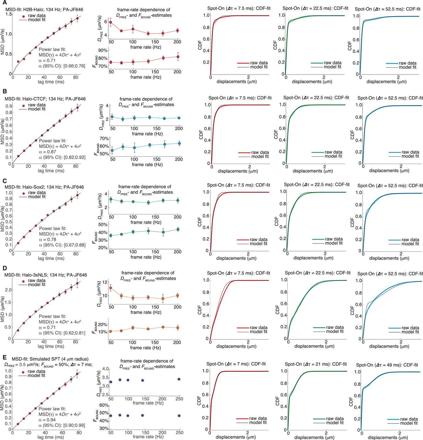
Sensitivity of Spot-On to anomalous diffusion.
(A) MSD-fit and Spot-On for U2OS H2B-Halo PA-JF646 spaSPT at 134 Hz. First column: A power law was fit to the time- and –ensemble-averaged mean squared displacement (MSD) and the anomalous diffusion exponent, α, inferred. To calculate the MSD from only the free population, vbSPT with an enforced 2-state model was used to classify trajectories into either bound or free and the MSD calculated from the vbSPT-classified free population. Error bars were obtained from jackknife sampling: random 50% subsamples of the data were taken, the MSD calculated and this repeated 20 times. Error bars show standard deviation among subsamplings. The best-fit α-value as well as 95% confidence intervals (CI) are shown. Second column: Spot-On inferred DFREE and FBOUND from spaSPT experiments at a range of frame rates from 50 Hz to 200 Hz. Despite anomalous diffusion, Spot-On is nevertheless able to estimate reasonably consistent DFREE and FBOUND across a wide range of frame-rates. Third to fifth column: Spot-On (JumpsToConsider = 4; 2-state model) CDF-fits at three selected time-points, showing that even with significant anomalous diffusion and only three fitted parameters, Spot-On can nonetheless fit the data reasonably well. (B) MSD-fit and Spot-On for U2OS C32 Halo-CTCF PA-JF646 spaSPT at 134 Hz. Each column is described in (A). (C) MSD-fit and Spot-On for mESC C3 Halo-Sox2 PA-JF646 spaSPT at 134 Hz. Each column is described in (A). (D) MSD-fit and Spot-On for U2OS Halo-3xNLS PA-JF646 spaSPT at 134 Hz. Each column is described in (A). (E) MSD-fit and Spot-On for simulated data with DFREE = 3.5 µm2/s; FBOUND = 50%; 7 ms per frame.
Figure 4—figure supplement 3
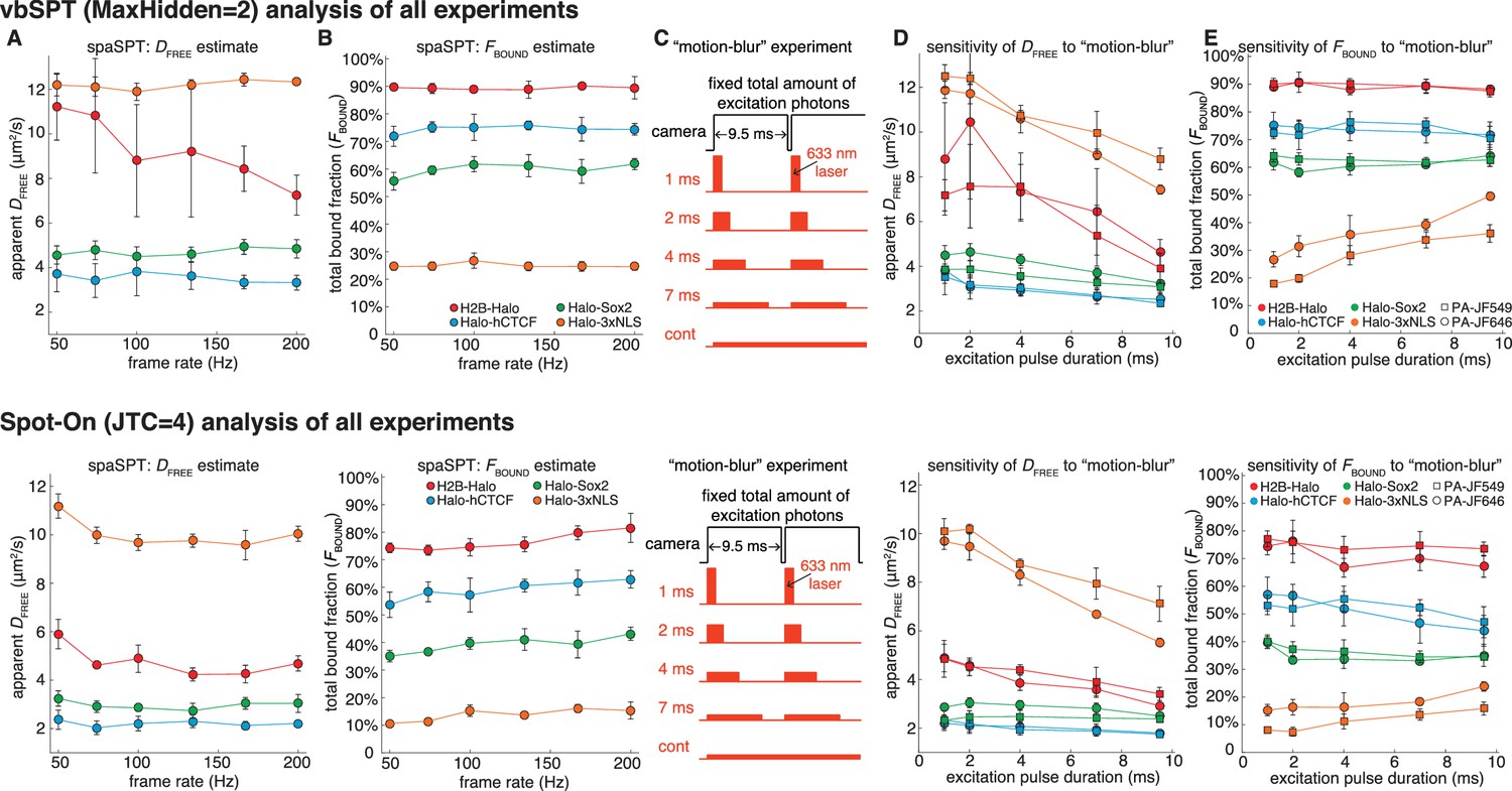
Re-analysis of experimental data using vbSPT.
We re-analyzed the experimental data shown in Figure 4G–K using vbSPT (allowing up to two states) instead of Spot-On. (A-B) Effect of frame-rate on DFREE and FBOUND. spaSPT was performed at 200 Hz, 167 Hz, 134 Hz, 100 Hz, 74 Hz and 50 Hz using the 4 cell lines and the data analyzed using vbSPT (max two states). Each experiment on each cell line was performed in four replicates on different days and ~5 cells imaged each day. Error bars show standard deviation between replicates. (C) Motion-blur experiment. To investigate the effect of ‘motion-blurring’, the total number of excitation photons was kept constant, but delivered during pulses of duration 1, 2, 4, 7 ms or continuous (cont) illumination. (D-E) Effect of motion-blurring on DFREE and FBOUND. spaSPT data was recorded at 100 Hz and the data analyzed using vbSPT (max two states). The inferred DFREE (D) and FBOUND (E) were plotted as a function of excitation pulse duration. Each experiment on each cell line was performed in four replicates on different days and ~5 cells imaged each day. Error bars show standard deviation between replicates. Compared to Spot-On (Figure 4G–K; repeated below), vbSPT generally reports a higher bound fraction (e.g. vbSPT reports a total bound fraction for Halo-Sox2 of ~60–65%, which is much higher than previously reported [Teves et al., 2016]). vbSPT most likely overestimates the bound fraction because it does not account for defocalization bias.
Author response image 1

Videos
Video 1
Related to Figure 1.
Illustration of defocalization bias. Illustration of a single-particle tracking experiment with two subpopulations (one ‘immobile’, D = 0.001 µm²/s, the other ‘free’, D = 4 µm²/s with a 1:1 ratio, observed using 20 ms time interval). The red region corresponds to the axial detection range (1 µm) and molecules randomly appear when they photo-activate. For each trajectory, the detected localizations inside the detection range are shown as red spheres and undetected localizations outside the detection range are shown as white spheres. Each particle has a mean lifetime of 15 frames, 25 nm localization error and trajectories consisting of at least two frames are plotted. Epi illumination is assumed. The SPT data was simulated and plotted using simSPT (available at https://gitlab.com/tjian-darzacq-lab/simSPT).
Video 2
Related to Figure 4.
Representative raw spaSPT movie (Halo-hCTCF at 134 Hz). spaSPT movie (1 ms of 633 nm laser delivered at the beginning of each frame; 405 nm laser photo-activation pulses delivered in between frames) of endogenously tagged CTCF (C32 Halo-hCTCF) in human U2OS cells imaged at ~134 Hz (7.477 ms per frame). Dye: PA-JF646. One pixel: 160 nm.
Tables
Table 1
Summary of simulation results and comparison of methods.
The table shows the bias (mean error), ‘std’ (standard deviation) and ‘iqr’ (inter-quartile range: difference between the 75th and 25th percentile) for each method for all 3480 simulations. The left column shows the relative bias/std/iqr for the DFREE-estimate and the right column shows the absolute bias/std/iqr for the FBOUND-estimate.
| Analysis method | DFREE | FBOUND | ||||
|---|---|---|---|---|---|---|
| bias | std | iqr | bias | std | iqr | |
| Spot-On (all) | −4.8% | 3.3% | 3.5% | −1.7% | 1.2% | 1.8% |
| vbSPT (2-state) | 0.8% | 12.5% | 6.8% | 5.0% | 4.6% | 6.1% |
| MSDi (R2 > 0.8) | 8.0% | 28.5% | 4.9% | −20.6% | 26.4% | 32.1% |
| MSDi (all) | −39.6% | 41.8% | 19.0% | 22.0% | 15.8% | 17.8% |
Key resources table
| Reagent type (species) or resource | Designation | Source or reference | Identifiers | Additional information |
|---|---|---|---|---|
| cell line (Homo sapiens) | Halo-CTCF | Hansen et al. eLife 2017;6:e25776; PMID 28467304; doi: 10.7554/eLife.25776 | U2OS C32 FLAG-Halo-CTCF | Previously reported homozygous endogenous knock-in cell line where all endogenous copies of CTCF have been N-terminally tagged with FLAG-HaloTag |
| cell line (Homo sapiens) | Halo-3xNLS | Hansen et al. eLife 2017;6:e25776; PMID 28467304; doi: 10.7554/eLife.25776 | U2OS Halo-3xNLS | U2OS cell line stably expressing Halo-3xNLS (3 copies of the SV40 Nuclear Localization Signal) generated by G418 selection. Generously provided by David T McSwiggen. |
| cell line (Homo sapiens) | H2B-Halo | Hansen et al. eLife 2017;6:e25776; PMID 28467304; doi: 10.7554/eLife.25776 | U2OS H2B-Halo-SNAP | U2OS cell line stably expressing histone H2B-Halo-SNAP generated by G418 selection. Generously provided by David T McSwiggen. |
| cell line (Mus musculus) | Halo-Sox2 | Teves et al. eLife 2016;5:e22280; PMID 27855781; doi: 10.7554/eLife.22280 | mESC JM8.N4 C3 Halo-FLAG-Sox2 | Previously reported homozygous endogenous knock-in cell line where both endogenous copies of Sox2 have been N-terminally tagged with HaloTag-FLAG. Generously provided by Sheila S Teves. |
| software, algorithm | Spot-On Matlab | this paper | Spot-On Matlab | Please see Materials and Methods for a full description. Open-source code is freely available at GitLab: : https://gitlab.com/tjian-darzacqlab/spot-on-matlab (copy archived at https://github.com/elifesciences-publications/spot-on-matlab) |
| software, algorithm | Spot-On Python | this paper | Spot-On Python | Please see Materials and Methods for a full description. Open-source code is freely available at GitLab: https://gitlab.com/tjian-darzacqlab/Spot-On-cli (copy archived at https://github.com/elifesciences-publications/spot-on-cli) |
| software, algorithm | Spot-On | this paper | Spot-On | Please see Materials and Methods for a full description. The web-interface can be found at https://spoton.berkeley.edu/ and the underlying source-code is freely available at GitLab: https://gitlab.com/tjian-darzacqlab/Spot-On (copy archived at https://github.com/elifesciences-publications/spot-on) |
| software, algorithm | simSPT | this paper | simSPT | Code for efficiently simulating experimentally realistic SPT data. Please see Materials and Methods for a full description. Open-source code is freely available at GitLab: https://gitlab.com/tjian-darzacq-lab/simSPT |
| software, algorithm | MSDi; vbSPT; | this paper and Persson et al. Nature Methods 2013; PMID: 23396281; DOI: 10.1038/nmeth.2367 | MSDi; vbSPT; | Supplementary software used for MSDi and vbSPT analysis as well as for generating the simulated data can be found at: https://zenodo.org/record/835171 |
| chemical compound, drug | PA-JF549 | Grimm et al. Nature Methods 2016; PMID 27776112; DOI: 10.1038/nmeth.4034 | PA-JF549 | Please contact Luke D Lavis for distribution. |
| chemical compound, drug | PA-JF646 | Grimm et al. Nature Methods 2016; PMID 27776112; DOI: 10.1038/nmeth.4034 | PA-JF646 | Please contact Luke D Lavis for distribution. |
Additional files
-
Supplementary file 1
PDF of step-by-step manual for using Spot-On.
- https://doi.org/10.7554/eLife.33125.025
-
Transparent reporting form
- https://doi.org/10.7554/eLife.33125.026
Download links
A two-part list of links to download the article, or parts of the article, in various formats.
Downloads (link to download the article as PDF)
Open citations (links to open the citations from this article in various online reference manager services)
Cite this article (links to download the citations from this article in formats compatible with various reference manager tools)
Robust model-based analysis of single-particle tracking experiments with Spot-On
eLife 7:e33125.
https://doi.org/10.7554/eLife.33125


