Routine single particle CryoEM sample and grid characterization by tomography
- Simons Electron Microscopy Center, New York Structural Biology Center, United States
- Columbia University, United States
- City College of New York, United States
- The Graduate Center of the City University of New York, United States
- National Institute of Allergy and Infectious Diseases, National Institutes of Health, United States
- Merck & Co., Inc, United States
Figures
Figure 1
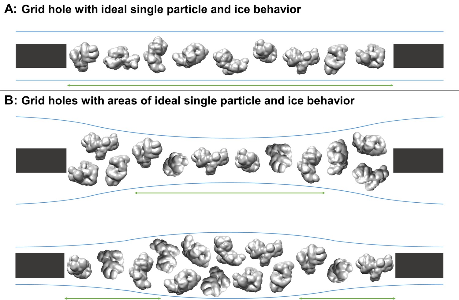
Schematic diagrams of grid hole cross-sections containing regions of ideal particle and ice behavior for single particle cryoEM collection.
(A) A grid hole where all regions of particles and ice exhibit ideal behavior. (B) Grid holes where there are areas that exhibit ideal particle and ice behavior. Green arrows indicate areas with ideal particle and ice behavior. The generic particle shown is a low-pass filtered holoenzyme, EMDB-6803 (Yin et al., 2017). The particles were rendered with UCSF Chimera (Pettersen et al., 2004).
Figure 2

Depictions of potential ice and particle behavior in cryoEM grid holes, based on Figure 6 from (Taylor and Glaeser, 2008).
A region of a hole may be described by a combination of one option from (A) for each air-water interface and one or more options from (B). An entire hole may be described by a set of regions and one or more options from (C). (A) Each air-water interface might be described by either (1), (2), or (3). Note that cryoET might only be able to resolve tertiary and secondary protein structures/network elements at the air-water interface. (B) Particle behavior between air-water interfaces and at each interface might be composed of any combination of (1) through (5), with or without aggregation. B3 is different from B4 if, for example, a particle prone to denaturation is frozen before or after denaturation has begun, thus potentially changing the set of preferred orientations. At high enough concentrations additional preferred orientations might become available in B3 and B4 due to neighboring protein-protein interactions. (C) Ice thickness variations through a central cross-section of hole may be described by one option for one air-water interface and one option for the apposed interface. Note that in C1 the particle's minor axis may be larger than the ice thickness. In both C1 and C4, the particle may still reside in areas thinner than its minor axis if the particle is compressible. Phenomenon such as bulging or doming (Brilot et al., 2012) may be represented as a combination of C1-4.
Figure 3
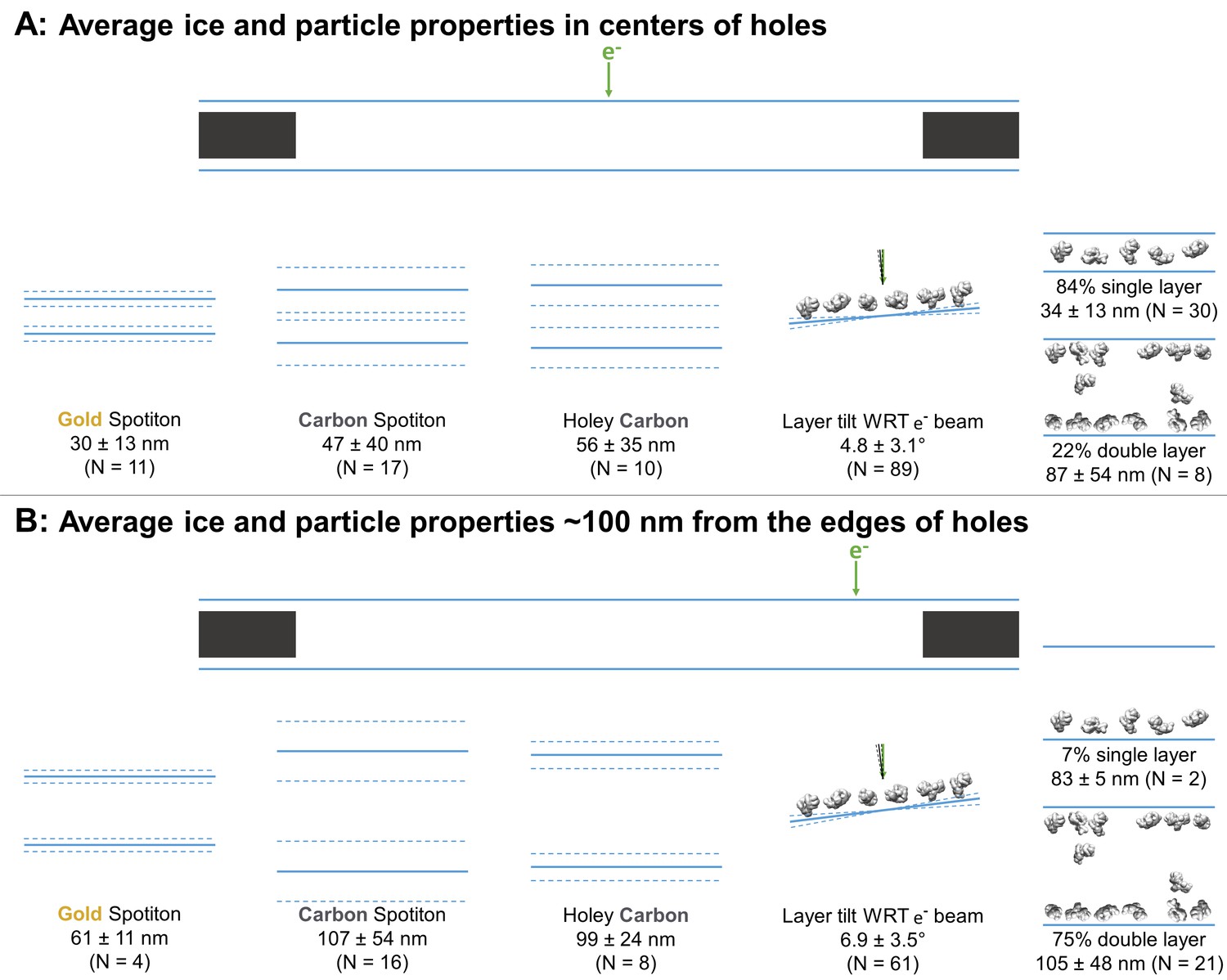
Schematic diagrams of the average ice thickness (solid lines) ± (1 standard deviation and measurement error) (dashed lines) using the minimum measured values, average particle layer tilt (solid lines) ± (1 standard deviation and measurement error) (dashed lines), and percentage of samples with single and/or double particle layers (‘1’ and/or ‘2’ as defined in Table 1) at the centers of holes (A) and about 100 nm from the edge of holes (B).
https://doi.org/10.7554/eLife.34257.006-
Figure 3—source data 1
Ice thickness and angle measurements for Figure 3.
- https://doi.org/10.7554/eLife.34257.007
Figure 4
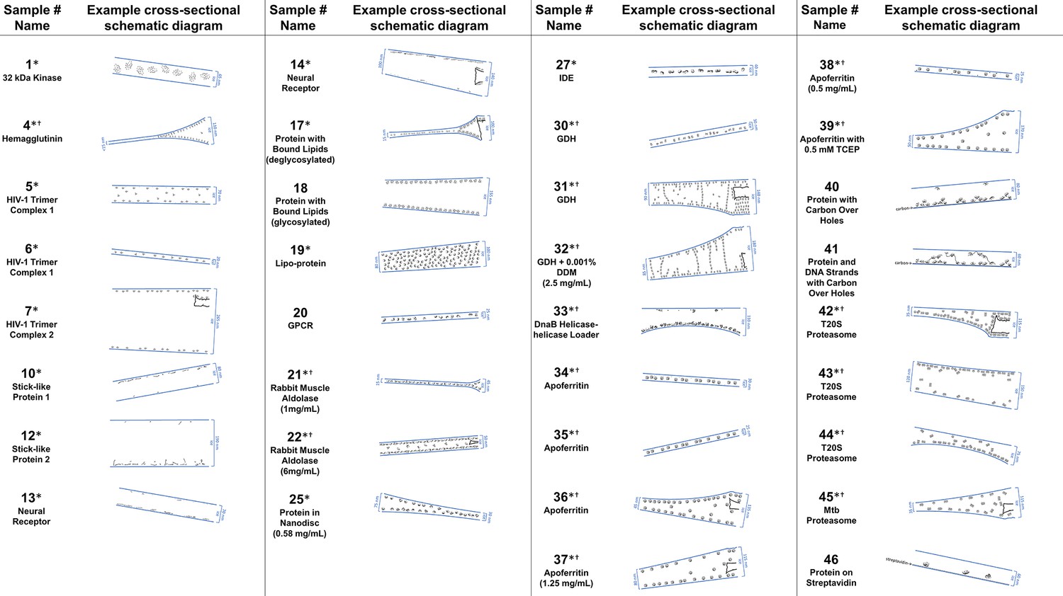
A selection of cross-sectional schematic diagrams of particle and ice behaviors in holes as depicted according to analysis of individual tomograms.
The relative thicknesses of the ice in the cross-sections are depicted accurately. Each diagram is tilted corresponding to the tomogram from which it is derived; i.e. the depicted tilts represent the orientation of the objects in the field of view at zero-degree nominal stage tilt. If the sample concentration in solution is known, then it has been included below the sample name. Black lines on schematic edges are the grid film. The cross-sectional characteristics depicted here are not necessarily representative of the aggregate. An asterisk (*) indicates that a Video of the schematic diagram alongside the corresponding tomogram slice-through video is included for the sample. A dagger (†) indicates that a dataset is deposited for sample. A generic particle, holoenzyme EMDB-6803 (Yin et al., 2017), is used in place of some confidential samples (samples #40, 41, and 46).
Figure 5
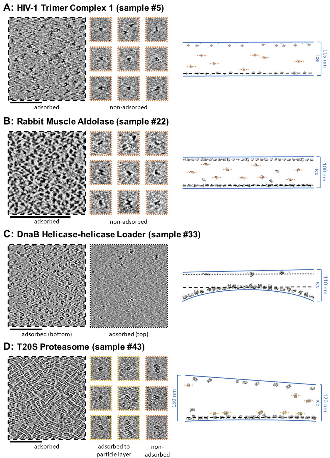
Slices of tomograms, about 7 nm thick, showing variations in particle orientation of adsorbed and non-adsorbed particles for several samples.
Cross-sectional schematic diagrams showing the approximate locations of the slices are shown on the right. (A) HIV-1 trimer complex 1 shows a high degree of preferred orientation for particles adsorbed to the air-water interface and no apparent preferred orientation for non-adsorbed particles. (B) Rabbit muscle aldolase shows several views for adsorbed particles and non-preferred views for non-adsorbed particles. (C) DnaB helicase-helicase loader shows no apparent preferred orientation for adsorbed particles. (D) T20S proteasome shows predominantly one view for adsorbed particles, the same view for particles adsorbed to the primary layer of particles, and less preferred views for non-adsorbed particles. Scale bars are 100 nm.
Figure 6
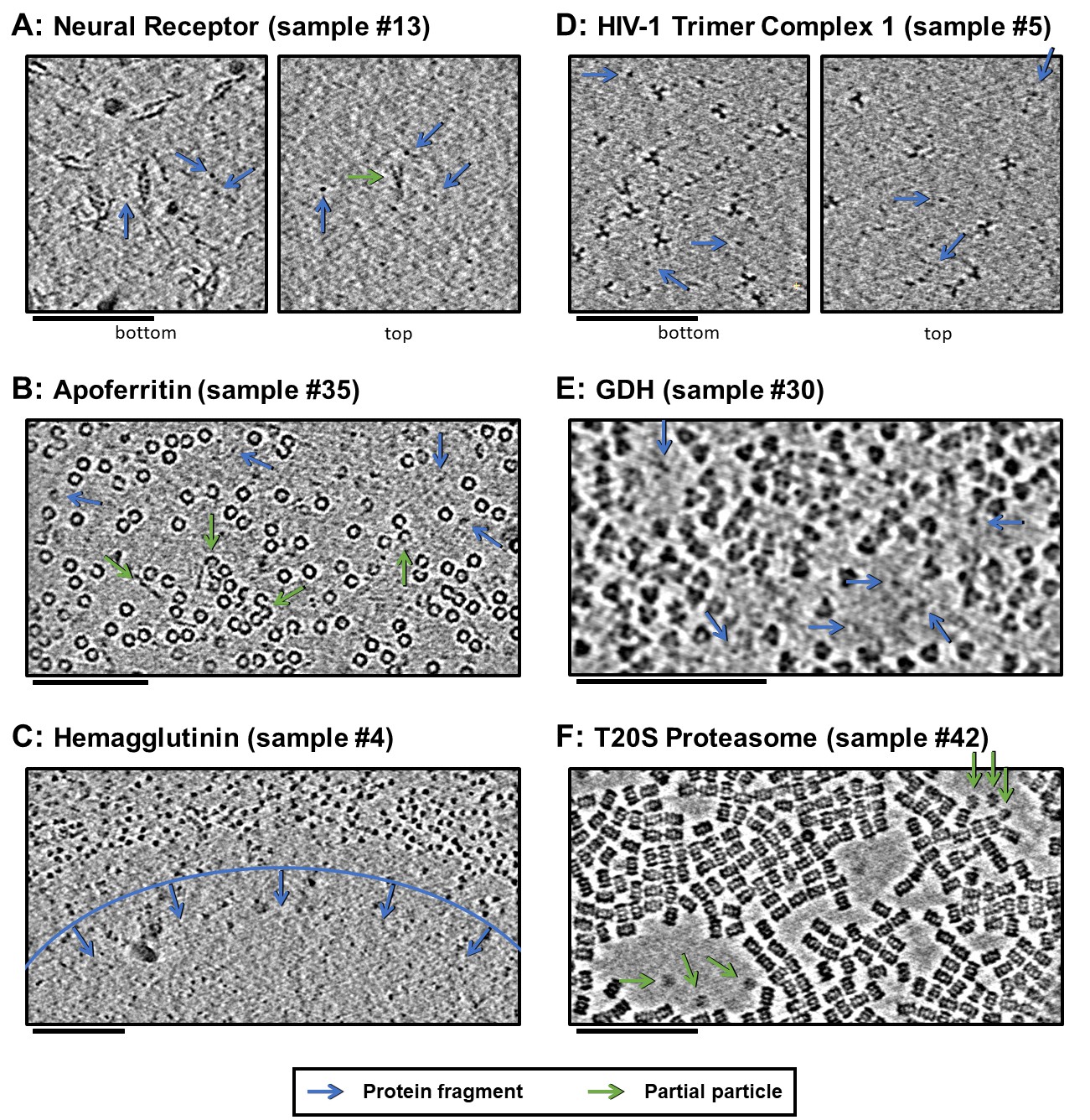
Slices of tomograms, about 10 nm thick, at air-water interfaces of samples that show clear protein fragments (examples indicated with blue arrows) and/or partial particles (examples indicated with green arrows), presented roughly in order of decreasing overall fragmentation.
(A) Neural receptor shows a combination of fragmented 13 kDa domains consisting primarily of β-sheets and partial particles. (B) Apoferritin shows apparent fragmented strands and domains along with partial particles. (C) Hemagglutinin shows a clear dividing line, marked with blue, where the ice became too thin to support full particles, but thick enough to support protein fragments. (D) HIV-1 trimer complex one shows several protein fragments on the order of 10 kDa; however, these might be receptors intentionally introduced to solution before plunge-freezing. (E) GDH shows protein fragments interspersed between particles. (F) T20S proteasome shows partial particles, determined by measuring their heights in the z-direction, on an otherwise clean air-water interface (see the end of Video 10 for sample #42). For the examples shown here, it is not clear whether the protein fragments and partial particles observed are due to unclean preparation conditions, protein degradation in solution, or unfolding at the air-water interfaces, or a combination; all cases are expected to result in the same observables due to competitive and sequential adsorption. Scale bars are 100 nm.
Figure 7
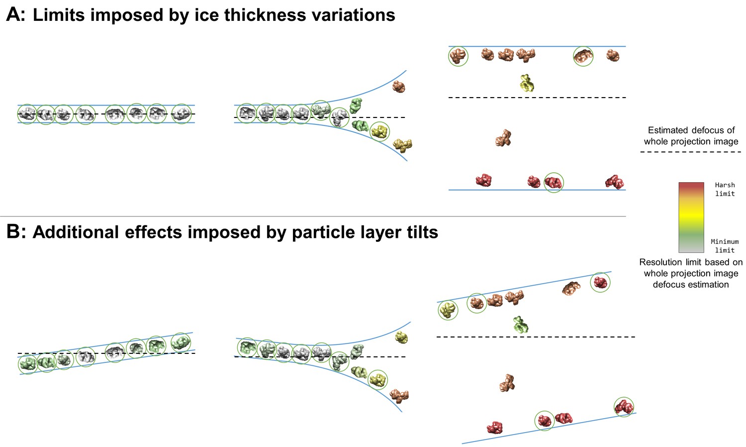
Collection and processing limits imposed by variations in ice thickness (A) and particle layer tilt (B), given that the vast majority of particles in holes on conventionally-prepared cryoEM grids are adsorbed to an air-water interface.
(A) Variations in ice thickness within and between holes might limit the number of non-overlapping particles in projection images (efficiency of collection and processing), the accuracy of whole image and local defocus estimation (accuracy in processing), the signal-to-noise ratio in areas of thicker ice (efficiency of collection and processing), and the reliability of particle alignment due to overlapping particles being treated as a single particle. (B) Variations in the tilt angle of a given particle layer might affect the accuracy of defocus estimation if the field of view is not considered to be tilted, yet will increase the observed orientations of the particle in the dataset if the particle exhibits preferred orientations. Dashed black lines indicate the height of defocus estimation on the projected cross-section if sample tilt is not taken into account during defocus estimation. Particles are colored relative to their distance from the whole image defocus estimation to indicate the effects of ice thickness and particle layer tilt. Gray particles would be minimally impacted by whole-image CTF correction while red particles would be harshly impacted by whole-image CTF correction. Particles that would be uniquely identifiable in the corresponding projection image are circled in green.
Figure 8
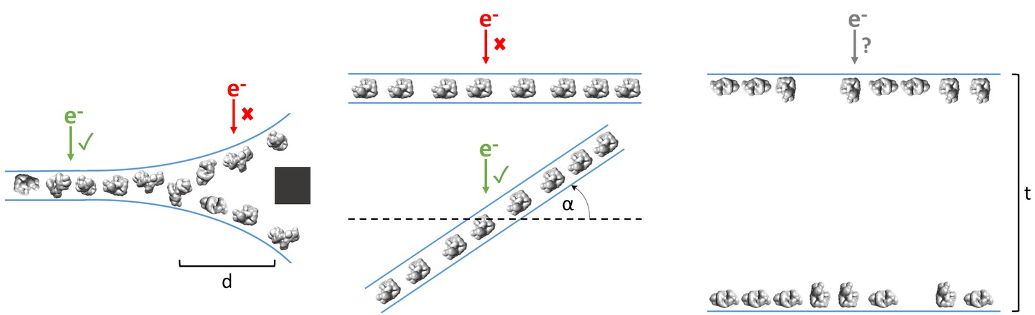
Examples of typical single particle and ice behavior as might be revealed by fiducial-less cryoET and how such characterization might influence strategies for single particle collection.
Left: For a sample that exhibits thick ice near the edges of holes and ice in the center of holes that is thin enough for a single layer of particles to reside, single particle micrographs would optimally be collected a distance, d, away from the edges of holes. Middle: A sample that exhibits a high degree of preferred orientation may require tilted single particle collection by intentionally tilting the stage by a set of angles, α, in order to recover a more isotropic set of particle projections (Tan et al., 2017). Right: For a sample that consists of multiple layers of particles across holes, the sample owner may decide to proceed with collection with the knowledge that the efficiency will be limited by the particle saturation in each layer and that the resolution will be limited by the decrease in signal due to the ice thickness, t, and the accuracy of CTF estimation and correction. The results of cryoET on a given single particle cryoEM grid might also result in the sample owner deciding that the entire grid is not worth collecting on, potentially due to the situations described here or due to observed particle degradation. Due to depiction limitations, the single orientation of the particle in the middle column is depicted as being only in one direction, when in practice the particles may rotate on the planes of the air-water interfaces.
Figure 9
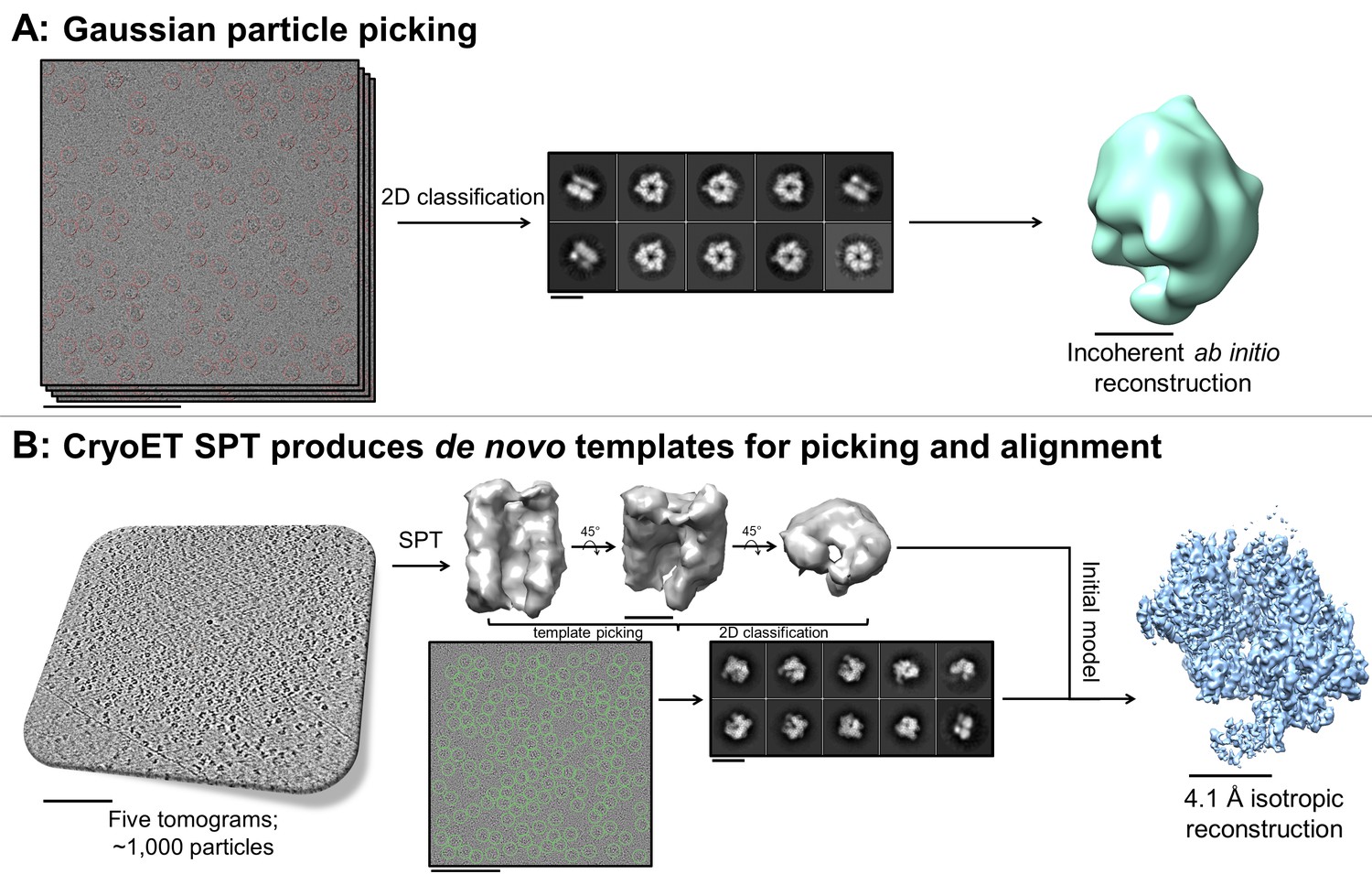
De novo initial model from fducial-less SPT.
(A) Gaussian picking of single particle datasets of DnaB helicase-helicase loader was not able to identify many low contrast side-views of the particle and 2D classification of the top-views incorrectly suggested C6 symmetry, resulting in unreliable initial model generation and stymying efforts to process the datasets further. (B) Fiducial-less single particle tomography (SPT) on the same grids used for single particle collection was employed to generate a de novo initial model, which was then used both as a template for picking all views of the particle in the single particle micrographs and as an initial model for single particle alignment, resulting in a 4.1 Å isotropic structure of DnaB helicase-helicase loader (manuscript in preparation). This exemplifies the novelty of applying this potentially crucial fiducial-less SPT workflow on cryoEM grids. Scale bars are 100 nm for the micrographs and tomogram, 10 nm for the 2D classes, and 5 nm for the 3D reconstructions.
Videos
Video 1
Sample 20.
https://doi.org/10.7554/eLife.34257.010
Video 2
Sample 34.
https://doi.org/10.7554/eLife.34257.012
Video 3
Sample 35.
https://doi.org/10.7554/eLife.34257.013
Video 4
Sample 36.
https://doi.org/10.7554/eLife.34257.014
Video 5
Sample 37.
https://doi.org/10.7554/eLife.34257.015
Video 6
Sample 38.
https://doi.org/10.7554/eLife.34257.016
Video 7
Sample 04.
https://doi.org/10.7554/eLife.34257.017
Video 8
Sample 05.
https://doi.org/10.7554/eLife.34257.018
Video 9
Sample 30.
https://doi.org/10.7554/eLife.34257.019
Video 10
Sample 42.
https://doi.org/10.7554/eLife.34257.020
Video 11
Sample 13.
https://doi.org/10.7554/eLife.34257.021
Video 12
Sample 12.
https://doi.org/10.7554/eLife.34257.022
Video 13
Sample 6.
https://doi.org/10.7554/eLife.34257.025
Video 14
Sample 7.
https://doi.org/10.7554/eLife.34257.026
Video 15
Sample 17.
https://doi.org/10.7554/eLife.34257.027
Video 16
Sample 33.
https://doi.org/10.7554/eLife.34257.029
Video 17
Sample 01.
https://doi.org/10.7554/eLife.34257.030
Video 18
Sample 10.
https://doi.org/10.7554/eLife.34257.031
Video 19
Sample 14.
https://doi.org/10.7554/eLife.34257.032
Video 20
Sample 19.
https://doi.org/10.7554/eLife.34257.033
Video 21
Sample 21.
https://doi.org/10.7554/eLife.34257.034
Video 22
Sample 22.
https://doi.org/10.7554/eLife.34257.035
Video 23
Sample 25.
https://doi.org/10.7554/eLife.34257.036
Video 24
Sample 27.
https://doi.org/10.7554/eLife.34257.037
Video 25
Sample 31.
https://doi.org/10.7554/eLife.34257.038
Video 26
Sample 32.
https://doi.org/10.7554/eLife.34257.039
Video 27
Sample 39.
https://doi.org/10.7554/eLife.34257.040
Video 28
Sample 43.
https://doi.org/10.7554/eLife.34257.041
Video 29
Sample 44.
https://doi.org/10.7554/eLife.34257.042
Video 30
Sample 45.
https://doi.org/10.7554/eLife.34257.043Tables
Table 1
Ice thickness measurements, number of particle layers, preferred orientation estimation, and distance of particle layers from the air-water interface as determined by cryoET of single particle cryoEM grids for 46 grid preparations of different samples.
The table is ordered in approximate order of increasing particle mass. Several particles are un-named as they are yet to be published. Sample concentration in solution is included with the sample name if known. Distance measurements are measured with an accuracy of a few nanometers due to binning of the tomograms by a factor of 4 and estimation of air-water interface locations using either contamination or particle layers. Grid types include carbon and gold holey grids and lacey and holey nanowire grids, plunged using conventional methods or with Spotiton. Edge measurements are made ~100 nm away from hole edges. ‘--’ indicates that these values were not measurable. Samples highlighted with blue contain regions of ice with near-ideal conditions (<100 nm ice, no overlapping particles, little or no preferred orientation). Samples highlighted with green contain regions of ice with ideal conditions (non-ideal plus no particle-air-water interface interactions). Incubation time for the samples on the grid before plunging is on the order of 1 s or longer.
| Sample # | Sample name | Grid type | Ice thickness (center, edge, substrate) in nm ± a few nm | # of Layers (center, edge, substrate) | Apparent preferred orientation in layer? | Min. particle/layer distance from air- water interface (nm ± a few nm) | ||||
|---|---|---|---|---|---|---|---|---|---|---|
| 1* | 32 kDa Kinase | Carbon Spotiton | 65 | 45 | -- | 0 | 0 | 0 | Unknown | <5 |
| 2 | 32 kDa Kinase | Gold Spotiton | 30 | -- | -- | 0 | -- | -- | Unknown | <5 |
| 3 | Insulin Receptor | Gold Spotiton | 55 | -- | -- | 1–2 | -- | -- | No | 5 |
| 4*† | Hemagglutinin | Carbon Spotiton | 25–95 | 100–210 | -- | 0 or 2 | 2 | -- | Some | 5 |
| 5* | HIV-1 Trimer Complex 1 | Carbon Spotiton | 75–210 | -- | -- | 2 | -- | -- | Yes | 5–10 |
| 6* | HIV-1 Trimer Complex 1 | Gold Spotiton | 20 | -- | -- | 1 | -- | -- | Some | 5 |
| 7* | HIV-1 Trimer Complex 2 | Carbon Spotiton | 190 | 265 | -- | 2 | 2 | 2 | Yes | 5 |
| 8 | 147 kDa Kinase | Gold Spotiton | 15 | -- | -- | 1 | -- | -- | Unknown | <5 |
| 9 | 150 kDa Protein | Holey Carbon Spotiton | 35 | 70 | -- | 2 | 2 | 2 | Some | <5 |
| 10* | Stick-like Protein 1‡ | Carbon Spotiton | 80 | -- | -- | 1 | -- | -- | No | <5 |
| 11 | Stick-like Protein 2 (150 kDa)‡ | Carbon CFlat | 100 | 100 | -- | 1 | 1 | -- | Unknown | 5 |
| 12* | Stick-like Protein 2‡ | Gold Spotiton | 135–190 | -- | -- | 1 | -- | -- | Some | 5 |
| 13* | Neural Receptor‡ | Carbon Spotiton | 60–90 | -- | -- | 1 | -- | -- | Yes | 5 |
| 14* | Neural Receptor‡ | Carbon Spotiton | 80–90 | 100–140 | 135 | 1 | 1 | 1 | Yes | 5 |
| 15 | 200 kDa Protein | CFlat Carbon + Gold mesh | 40–60 | 95 | 110 | 1 | 1 | 2 | No | 5 |
| 16 | Small, Popular Protein | Carbon Spotiton | 30 | 70 | -- | 1 | 2 | 2 | No | 5 |
| 17* | Glycoprotein with Bound Lipids (deglycosylated) | Carbon Spotiton | 15 | 90 | 130 | 1 | 2 | 2 | Yes | <5 |
| 18 | Glycoprotein with Bound Lipids (deglycosylated)‡ | Gold Spotiton | 155 | -- | -- | 2 | -- | -- | Some | <5 |
| 19* | Lipo-protein | Holey Carbon | 0–95 | 85–100 | -- | Uniformly distributed in ice | Unknown | 5 | ||
| 20* | GPCR | Carbon Spotiton | 25 | -- | -- | 1 | 2 | -- | No | 5 |
| 21*† | Rabbit Muscle Aldolase (1 mg/mL) | Gold Spotiton | 15 | 50 | -- | 1 | 2 | -- | No | <5 |
| 22*† | Rabbit Muscle Aldolase (6 mg/mL) | Carbon Spotiton | 60–110 | 75–130 | 85 | 2 | 2 | 2 | Some | 5 |
| 23 | Un-named Protein | Holey Carbon | 35 | -- | 60 | 1 | -- | 2 | Yes | 5 |
| 25* | Protein in Nanodisc (0.58 mg/mL) | Gold Spotiton | 30 | 65 | -- | 1–2 | 2 | -- | No | 5–10 |
| 26 | IDE | Carbon Spotiton | 25 | 60 | 95 | 1 | 2 | 2 | Unknown | 5 |
| 27* | IDE | Gold Spotiton | 40 | -- | -- | 1 | -- | -- | No | 5–10 |
| 28 | Small, Helical Protein | Gold Spotiton | 50 | 75 | -- | 1 | 2 | -- | Some | 5 |
| 29 | 300 kDa Protein | Carbon Spotiton | 30 | 100 | -- | 1 | 2 | 2 | No | 5 |
| 30*† | GDH | Holey Carbon | 30 | 85 | 100 | 1 | 1 | 3 | Some | 5 |
| 31*† | GDH | Holey Carbon | 60 | 120 | 140 | 1 | 2 | 3 | Yes | 5 |
| 32*† | GDH (2.5 mg/mL)+0.001% DDM | Carbon Spotiton | 50 | 180 | 190 | 1 | 2 | -- | Yes | <5 |
| 33*† | DnaB Helicase-helicase Loader | Gold Quantifoil | 50–55 | 80–100 | -- | 1 | 2 | -- | No | 5 |
| 34*† | Apoferritin | Gold Spotiton | 25–30 | -- | -- | 1 | -- | -- | No | 5 |
| 35*† | Apoferritin | Gold Spotiton | 25 | -- | -- | 1 | -- | -- | No | 5 |
| 36*† | Apoferritin | Holey Carbon Spotiton | 30 | 125 | 135 | 1 | 2 | 2 | No | 5 |
| 37*† | Apoferritin (1.25 mg/mL) | Holey Carbon Spotiton | 30–50 | 100 | 105 | 1 | 2 | 2 | No | 5 |
| 38*† | Apoferritin (0.5 mg/mL) | Holey Gold Spotiton | 25–30 | 55 | -- | 1 | 2 | -- | No | <5 |
| 39*† | Apoferritin with 0.5 mM TCEP | Carbon Spotiton | 40–90 | 145–175 | -- | 1–2 | 2 | 1 | No | 5 |
| 40 | Protein with Carbon Over Holes | Carbon Quantifoil | 110 | 70–100 | -- | 1 | 1 | -- | Some | 5–10 |
| 41 | Protein and DNA Strands with Carbon Over Holes | Carbon Quantifoil | 60 | -- | -- | 1 | -- | -- | Some | 5–10 |
| 42*† | T20S Proteasome | Holey Carbon | 35 | 115 | 120 | 1 | 2 | 3 | Some | <5 |
| 43*† | T20S Proteasome | Holey Carbon | 125 | 140–160 | 150 | 2 | 2 | 2 | Some | 5 |
| 44*† | T20S Proteasome | Gold Quantifoil | 50–75 | -- | -- | 1 | -- | -- | Some | 5 |
| 45*† | Mtb 20S Proteasome | Carbon Spotiton | 35 | 80 | 115 | 0 | 1 | 1 | No | 5–10 |
| 46 | Protein on Streptavidin | Holey Carbon | 20–100 | 80–120 | -- | 0–2 | 1–2 | -- | No | 10 |
-
*A video is included for this sample.
†A dataset is deposited for this sample.
-
‡Intentionally thick ice.
Table 2
Apparent air-water interface, particle, and ice behavior of the same samples in Table 1 using the descriptions in Figure 1.
Tilt-series were aligned and reconstructed using the same workflow and thus are oriented in the same direction. However, the direction relative to the sample application is not known. The bottom air-water interface corresponds to lower z-slice values, and the top to higher z-slice values as rendered in 3dmod from the IMOD package (Kremer et al., 1996). ‘A’ means that the air-water interface is apparently clean and cannot be visually differentiated between A1, A2 (primary structure), or A3. Percentages in parentheses are particle layer saturation estimates. Reported angles are the angles (absolute value) between the particle layer’s normal and the electron beam direction, measured using ‘Slicer’ in 3dmod. It is often difficult to distinguish between flat and curved ice at the air-water interfaces (e.g. Figure 2, ‘C1 or C2’ or ‘C2 or C3’) because most fields of view do not span entire holes. ‘‡’ indicates that the top layer of objects is the same layer as the bottom layer. ‘--’ indicates that these values were not measurable.
| Sample # | Sample name | Air-water interface, particle behavior, and layer/ice angle (bottom, center) | Air-water interface, particle behavior, and layer/ice angle (bottom, edge) | Ice behavior (bottom) | Air-water interface, particle behavior, and layer/ice angle (top, center) | Air-water interface, particle behavior, and layer/ice angle (top, edge) | Ice behavior (top) | Notes |
|---|---|---|---|---|---|---|---|---|
| 1* | 32 kDa Kinase | A, B1 or B2 or B3 (50%), 8° | A, B1 or B2 or B3 (50%), 10° | C2 | A, B1 or B2 or B3‡ (50%), 8° | A, B1 or B2 or B3‡ (50%), 10° | C2 | Particles aggregate into clouds. |
| 2 | 32 kDa Kinase | A, B1 or B2 or B3 (50%), 4–8° | -- | C1 or C2 | A, B1 or B2 or B3‡ (50%), 4–8° | -- | C1 or C2 | Gold beads are glow discharge contamination. |
| 3 | Insulin Receptor | A, B1 or B2 or B3 (100%), 3–5° | -- | C2 or C3 | A, B1 or B2 or B3‡ (100%), 3–5° | -- | C2 or C3 | Gold beads are glow discharge contamination. |
| 4*† | Hemagglutinin | A2, No particles, 3–7° | A, B3 (40%), 5° or A, B3 (40%), 3° | C3 or C4 | A2‡, No particles, 3–7° or A, B3 (50%), 7° | A, B3 (50%), 5–7° | C3 or C4 | Where very thin ice in the center of holes excludes particles, protein fragments remain. |
| 5* | HIV-1 Trimer Complex 1 | A2, B1, B3 (30%), 1–5° | -- | C1, C2, or C3 | A2, B1, B3 (30%), 1–5° | -- | C1, C2, or C3 | Trimer domains and/or unbound receptors are adsorbed to air-water interfaces. |
| 6* | HIV-1 Trimer Complex 1 | A2, B3 (80%), 6° | -- | C2 | A2, B3‡ (80%), 6° | -- | C2 | Trimer domains and/or unbound receptors are adsorbed to air-water interfaces. |
| 7* | HIV-1 Trimer Complex 2 | A, B2 or B3 (50%), 1° | A, B2 or B3 (50%), 3° | C1 or C2 | A, B2 or B3 (70%), 1° | A, B2 or B3 (70%), 3° | C1 or C2 | |
| 8 | 147 kDa Kinase | A, B2 or B3 (50%), 0° | -- | C2 or C3 | A, B2 or B3‡ (50%), 0° | -- | C2 or C3 | Gold beads are glow discharge contamination. |
| 9 | 150 kDa Protein | A, B2 or B3 (60%), 7–10° | A, B2 or B3 (60%), 8° | C2 or C3 | A, B2 or B3‡ (60%), 7° | A, B2 or B3 (40%), 9° | C2 or C3 | |
| 10* | Stick-like Protein 1 | A and A2, B4 and B5 (1%), 10° | -- | C2 | A2, B4 and B5 (50%), 10° | -- | C2 | |
| 11 | Stick-like Protein 2 (150 kDa) | A2, B3 and B4 and B5 (70%), 7° | A2, B3 and B4 and B5 (70%), 7° | -- | A2, B3 and B4 and B5‡ (70%), 7° | A2, B3 and B4 and B5‡ (70%), 7° | -- | Determinations are not accurate due to over focusing and minimal tilt angles. |
| 12* | Stick-like Protein 2 | A2, B3 (80%), 0° | -- | C2 or C3 | A2, B3 (1%), 0° | -- | C2 or C3 | Note 1. Note 2. |
| 13* | Neural Receptor | A2, B3 (80%), 3–10° | -- | C2 or C3 | A2, No particles, 3–10° | -- | C2 or C3 | Note 1. Note 2. |
| 14* | Neural Receptor | -- | A2, No particles, 2–7° or A2, B3 (70%), 5° | C3 | -- | A2, B3 (70%), 7° or A2, No particles, 7° | C3 | Note 1. Note 2. Two tomograms have one orientation, one has the opposite. |
| 15 | 200 kDa Protein | A, B2 or B3 (60%), 2° | A, B2 or B3 (50%), 4° | C3 | No particles or A, B2 or B3‡ (60%), 2° | A, No particles, 11° | C3 | |
| 16 | Small, Popular Protein | A, B2 or B3 (90%), 6° | A, B2 or B3 (90%), 9° | C2 | A, B2 or B3‡ (90%), 6° | A, B2 or B3 (90%), 1° | C3 | |
| 17* | Glycoprotein with Bound Lipids (deglycosylated) | A, B3 (70%), 4° | A, B3 (80%), 10° | C3 | A, B3‡ (70%), 4° | A, B3 (80%), 11° | C3 | Lipid membrane dissociates from protein in center. |
| 18 | Glycoprotein with Bound Lipids (glycosylated) | A, B3 (50%), 10° | -- | C2 or C3 | A, B3 (60%), 4° | -- | C2 or C3 | |
| 19* | Lipo-protein | No particles or A, B2, 3° | A, B3, 11° | C3, C4 | No particles or A, B2‡, 5° | A, B3, 11° | C3, C4 | Particles are uniformly distributed in the ice. |
| 20* | GPCR | A, B2 or B3 (70%), 3° | A, B2 or B3 (60%), -- | C3 | A, B2 or B3‡ (70%), 3° | A, B2 or B3 (60%), -- | C3 | |
| 21*† | Rabbit Muscle Aldolase (1 mg/mL) | A, B2 or B3 (90%), 3–9° | A, B2 or B3 (80%), 6° | C3 | A, B2 or B3‡ (90%), 3–9° | A, B2 or B3 (80%), 10° | C3 | |
| 22*† | Rabbit Muscle Aldolase (6 mg/mL) | A, B1, B2 or B3 (90%), 5° | A, B1, B2 or B3 (90%), 5° | C2 or C3 | A, B1, B2 or B3 (90%), 5° | A, B1, B2 or B3 (90%), 5° | C2 or C3 | |
| 23 | Un-named Protein | A, B3 (40%), 0–3° | -- | C2 or C3 | A, B3‡ (40%), 0–3° | -- | C2 or C3 | |
| 24 | Un-named Protein | A, B3 (80%), 2° | A, B3 (60%), 4–6° | C3 | A, B3‡ (80%), 2° | A, B3 (60%), 4–9° | C3 | |
| 25* | Protein in Nanodisc (0.58 mg/mL) | A, B2 (80%), 8–10° | A, B2 (80%), 8–10° | C2 or C3 | A, B2‡ (80%), 8–10° | A, B2 (80%), 8–10° | C2 or C3 | |
| 26 | IDE | A2, B2 or B3 and B4 and B5 (50%), 0° | A2, B1, B2 or B3 and B4 and B5 (50%), 5° | C3 | A2, B2 or B3 and B4 and B5‡ (50%), 0° | A2, B1, B2 or B3 and B4 and B5 (50%), 2° | C3 | Note 1. |
| 27* | IDE | A, B2 or B3 (95%), 0–4° | -- | C2 | A, B2 or B3 (95%), 0–4° | -- | C2 | |
| 28 | Small, Helical Protein | A, B2 or B3 (80%), 5° | A, B2 or B3 (70%), 3° | C3 | A, B2 or B3‡ (80%), 5° | A, B2 or B3 (70%), 7° | C3 | |
| 29 | 300 kDa Protein | A or A2, B2 or B3 (70%), 7° | A or A2, B2 or B3 (50%), 13° | C3 | A or A2, B2 or B3‡ (70%), 7° | A or A2, B2 or B3 (50%), 9° | C3 | |
| 30*† | GDH | A, B3 (70%), 10° | A, B1, B3 (50%), 1° | C2 | A, B3‡ (70%), 10° | A, B1, B3 (50%), 16° | C3 | Note 2. Some non-adsorbed particles stack between layers. |
| 31*† | GDH | A, B3 (40%), -- | A, B1, B3 (40%), 10° | C3 | A, B3‡ (40%), -- | A, B1, B3 (40%), 2° | C2 | |
| 32*† | GDH (2.5 mg/mL)+0.001% DDM | A, B3 (40%), 4° | A, B1, B3 (40%), 7° | C2 | A, B3‡ (30%), 4° | A, B1, B3 (30%), 6° | C3 | Some non-adsorbed particles stack between layers. |
| 33*† | DnaB Helicase-helicase Loader | A, B2 or B3 (90%), 1° | A, B2 or B3 (90%), 4° | C3 | A, B2 or B3 (<5%), 1° | A, B2 or B3 (<5%), 1° | C2 | Gold flakes from Quantifoil are on the top. |
| 34*† | Apoferritin | A2, B2 or B3 (50%), 4–6° | -- | C2 or C3 | A2, B2 or B3‡ (50%), 4–6° | -- | C2 or C3 | Note 1. Note 2. |
| 35*† | Apoferritin | A2, B2 or B3 (60%), 4–12° | -- | C2 or C3 | A2, B2 or B3‡ (60%), 4–12° | -- | C2 or C3 | Note 1. Note 2. |
| 36*† | Apoferritin | A2, B3 (50%), 5° | A2, B1, B3 (50%), 10° | C3 | A2, B3‡ (70%), 5° | A2, B1, B3 (60%), 3° | C3 | Note 1. Note 2. |
| 37*† | Apoferritin (1.25 mg/mL) | A2, B2 or B3 (50%), 4–7° | A2, B1, B2 or B3 (50%), 6° | C3 | A2, B2 or B3‡ (40%), 4° | A2, B1, B2 or B3 (30%), 4° | C3 | Note 1. Note 2. |
| 38*† | Apoferritin (0.5 mg/mL) | A2, B2 or B3 (20%), 5° | -- | C2 or C3 | A2, B2 or B3‡ (20%), 1° | -- | C2 or C3 | Note 1. Note 2. |
| 39*† | Apoferritin with 0.5 mM TCEP | A, B2 or B3 (40%), -- or A, B2 or B3 (50%), 3° | A, B1, B2 or B3 (40%), 5–9° | C3 | A, B2 or B3 (40%), -- or A, B2 or B3‡ (50%), 3° | A, B1, B2 or B3 (40%), 2–8° | C3 | Note 1. Note 2. |
| 40 | Protein with Carbon Over Holes | Carbon, B1 (30%), B3 (60%), 5° | Carbon, B1 (30%), B3 (60%), 5–9° | C2 | A, B3 (5%), 5° | A, B3 (5%), 5° | C1 or C2 | Note 3. |
| 41 | Protein and DNA Strands with Carbon Over Holes | A, No particles, 2–3° | -- | C2 or C3 | Carbon, B1 (20%), B3 (60%), 2–3° | -- | C2 | Some non-adsorbed particles make contact with particle layer. Most non-adsorbed particles are attached to DNA strands. |
| 42*† | T20S Proteasome | A, B3 (80%), 3° | A, B1 (5%), B3 (80%), 14° | C3 | A, B3‡ (80%), 3° | A, B1 (5%), B3 (20%), 3° | C2 | Note 2. Note 3. |
| 43*† | T20S Proteasome | A, B3 (10%), 2–5° | A, B3 (10%), 2–5° | C2 | A, B1 (20%), B3 (90%), 5–7° | A, B1 (20%), B3 (95%), 5–7° | C3 | Note 3. |
| 44*† | T20S Proteasome | A, B1 (10%), B3 (80%), 11° | -- | C3 | A, B3 (2%), 11° | -- | C2 | Note 2. Note 3. |
| 45*† | Mtb 20S Proteasome | -- | A, B1, B2 or B3 (30%), 6° | C3 | -- | A, B1, B2 or B3 (30%), 11° | C3 | Heavy contamination. |
| 46 | Protein on Streptavidin | Streptavidin, B2 (10–30%), 0° or Streptavidin, No particles, 12° | Streptavidin or A2, 2 (10–30%), 12° | C1, C2, or C3 | Streptavidin, B2 (10–30%), 0° or Streptavidin‡, No particles, 12° | Streptavidin, 2 (10–30%), 13–14° | C1, C2, or C3 | Note 1. Some holes have a layer of streptavidin only on top, some have a layer on top and bottom. Particles are attached to streptavidin and sometimes the apposed air-water interface. |
-
*A video is included for sample.
†A dataset is deposited for sample.
-
Note 1: Apparent protein fragments/domains are adsorbed to the air-water interfaces.
Note 2: Partial particles exist.
-
Note 3: Non-adsorbed particles make contact with particle layer.
Additional files
-
Transparent reporting form
- https://doi.org/10.7554/eLife.34257.044
Download links
A two-part list of links to download the article, or parts of the article, in various formats.
Downloads (link to download the article as PDF)
Open citations (links to open the citations from this article in various online reference manager services)
Cite this article (links to download the citations from this article in formats compatible with various reference manager tools)
Routine single particle CryoEM sample and grid characterization by tomography
eLife 7:e34257.
https://doi.org/10.7554/eLife.34257


