Figures and data in Automated analysis of long-term grooming behavior in Drosophila using a k-nearest neighbors classifier

Figures
Videos
Tables
Additional files

8 figures, 4 videos, 3 tables and 1 additional file

Figures

Figure 1

Download asset Open asset

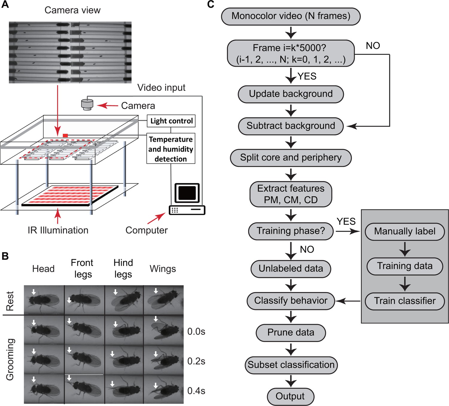
Overview of approach for detecting *Drosophila* grooming.

(A) Apparatus used in recording behavior. Flies constrained to individual tubes are continuously illuminated by infrared light from below and recorded by a digital camera from above. LED lights on sides of chamber simulate day-night light conditions. Temperature and humidity probes placed in the chamber are monitored by a computer. Inset: Camera photo of fly tubes in chamber. (B) Examples of the most commonly observed types of grooming in our experiments. The top row displays postures of a fly in inactive state. The three rows below show how the limbs and body of a fly coordinate to perform specific grooming movements. Arrows point to the moving part during grooming. (C) Flowchart of our algorithm used to classify fly behavior. After generating a suitable background image, the algorithm characterizes movements of fly center (CD), core (CM) and periphery (PM) to fully classify behavior in each frame.

https://doi.org/10.7554/eLife.34497.003

Figure 2 with 1 supplement

Download asset Open asset

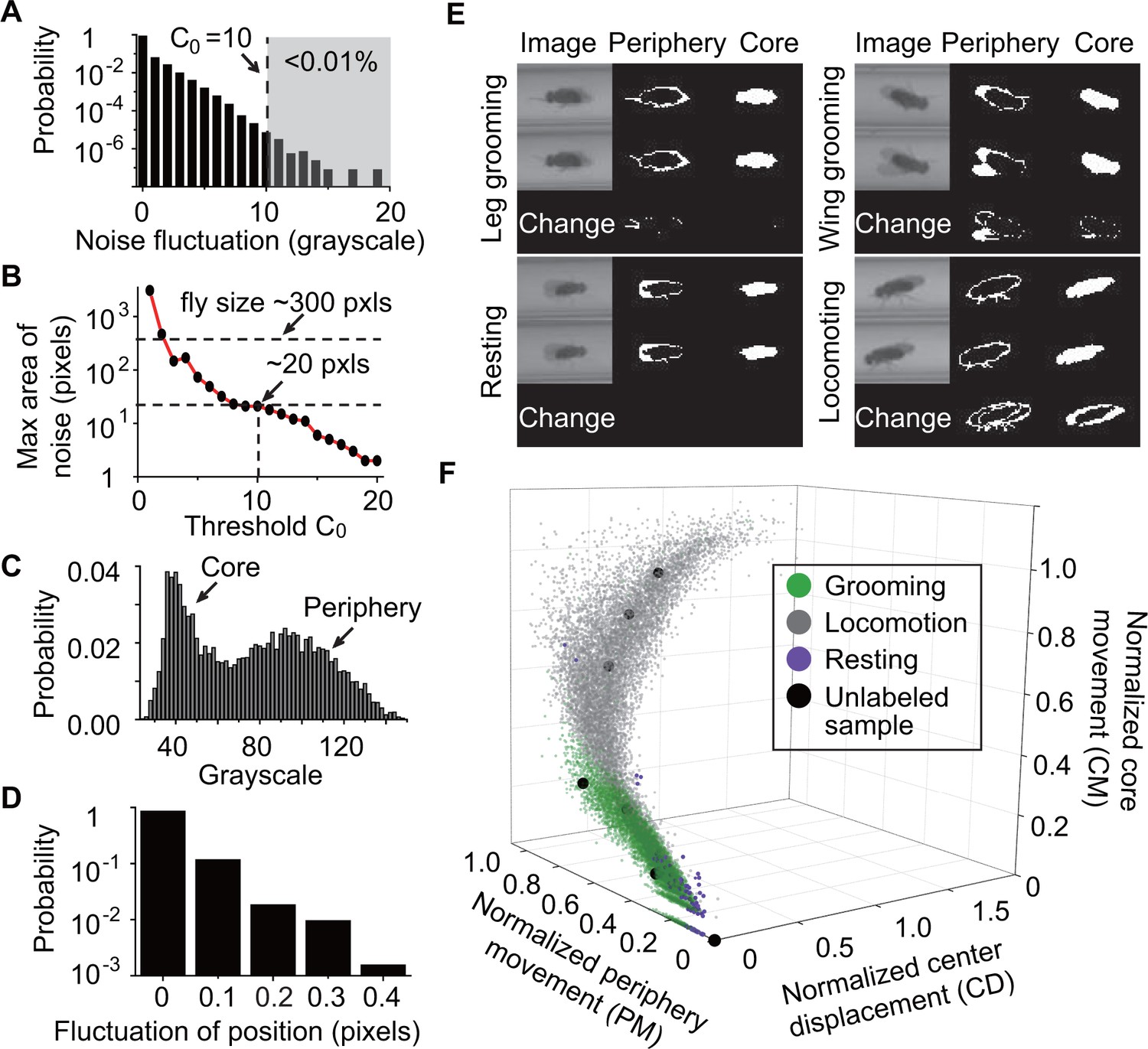
Feature extraction and behavior classification.

(A) The distribution of grayscale fluctuations in the absence of mobile flies. A cutoff of grayscale value change $C_{0}$ = 10 rules out >99.99% of fluctuations. Shown here are only positive values of fluctuations, which are symmetric about zero. (B) Maximum area (pixels) of a closed object generated by noise when different threshold $C_{0}$ are applied. A $C_{0}$ = 10 rejects objects larger than 20 pixels. Based on this, we set a threshold $C_{1}$ = 25 to remove objects smaller than 25 pixels without affecting identification of flies which have a typical area of ~300 pixels in our studies. (C) Grayscale value distribution of pixels belonging to 20 individual flies. Two regions are clearly seen: the left region with peak around 40 represents the core of the flies and the right region with peak around 90 represents their periphery. (D) Variations in the center position of a stationary fly. The minimum displacement that represents a true fly center movement is 0.5-pixel length in our experiment, a requirement that excludes >99.99% of false displacements. (E) Examples of original and processed images of a fly displaying different behaviors: Top, left: front leg grooming; top, right: wing grooming; bottom, left: resting; bottom, right: locomoting. In each panel, original images from two consecutive frames are shown on left, periphery in the middle and core on the right. Changes of periphery and core are shown in the bottom row. PM and CM denote differences in the number of pixels representing the fly periphery and core, respectively, in two frames. Features PM and CM are different for different behaviors. Rubbing of front legs manifests through PM (top, left) while sweeping wings affects PM and CM (top, right). (F) k-nearest neighbors (kNN) algorithm works by placing an unclassified sample (black circle) representing a frame into a feature space with pre-labeled samples (green/gray/purple circles, the training set). The label of the unclassified point is decided by the most frequent label among its k-nearest neighbors. The three axes of the feature space are normalized periphery movement (PM), core movement (CM), and center displacement (CD). Fly activity in the feature space is separated into three regions: grooming (green), locomotion (gray) and resting (purple). Training samples (N = 9322 grooming, 9930 locomotion, 5748 rest) and nine unlabeled samples in PM-CM-CD space are shown.

https://doi.org/10.7554/eLife.34497.007

Figure 2—source data 1 Source data for Figure 2.: https://doi.org/10.7554/eLife.34497.009
Download elife-34497-fig2-data1-v2.xlsx
Figure 2—source data 2 Source data for Figure 2—figure supplement 1.: https://doi.org/10.7554/eLife.34497.010
Download elife-34497-fig2-data2-v2.xlsx

Figure 2—figure supplement 1

Download asset Open asset

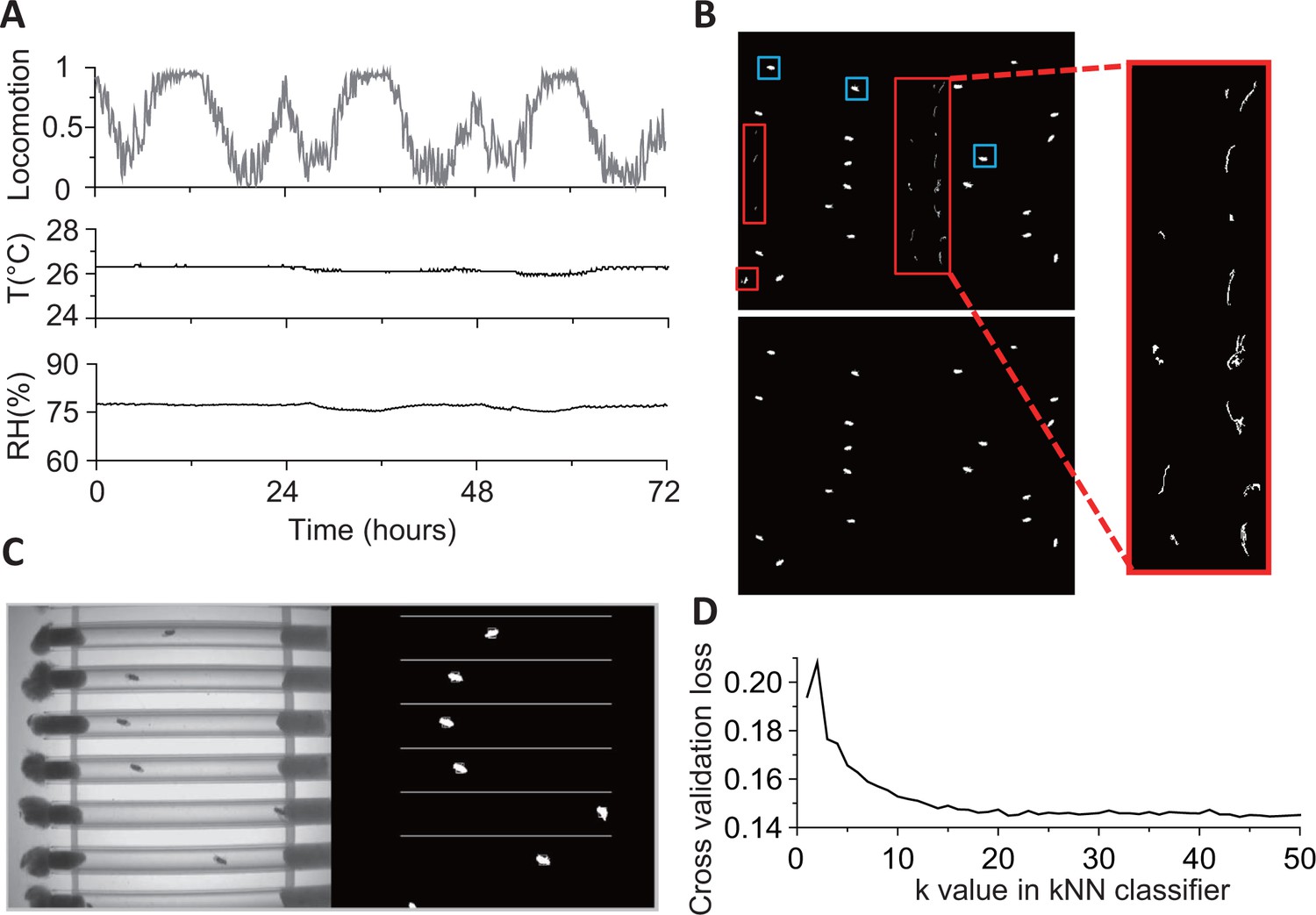
Details of environmental conditions and fly detection.

(A) Locomotion (fraction of time spent), relative humidity (RH), and temperature (T) for 3 days during an experiment in constant darkness (DD) conditions. Data are binned in 5 min. (B) Binary images after background subtraction. If the background frame is not updated frequently (typically every 1000 s), both food debris (red boxes) and flies (blue boxes) may be identified as moving objects in a background-subtracted image (top, left and expanded view). The problem is rectified (bottom, left) when the background frame used is closer in time (<1000 s apart) to the image of interest. (C) An example 8-bit frame (on left) and its corresponding background-subtracted binary image showing identified flies. (D) The cross-validation loss of kNN classifier at different k values. Loss decreases with increasing k values, slowing down for k $\approx$ 10. The loss function shown here is the averaged error of 10-fold cross validation in behavioral classification. The validation was performed on 25,000 frames from video of 20 flies.

https://doi.org/10.7554/eLife.34497.008

Figure 3

Download asset Open asset

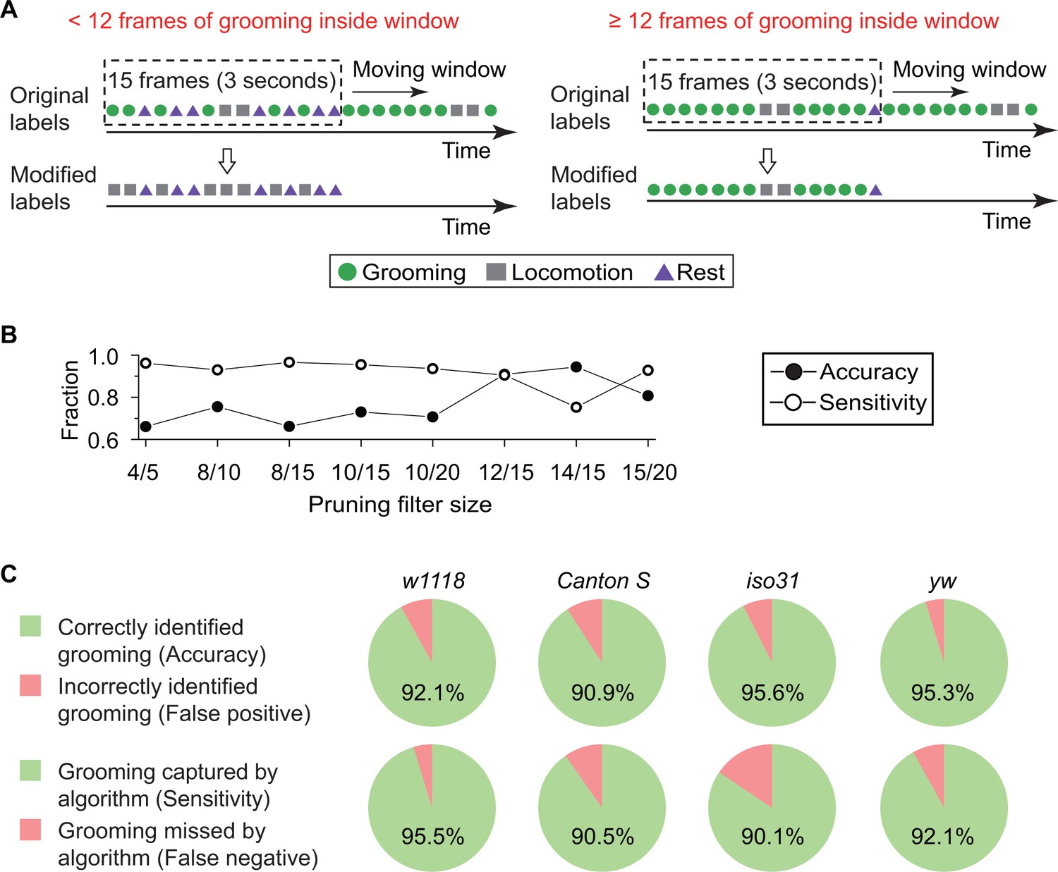
Data pruning and performance evaluation.

(A) Grooming data are pruned after identification by the kNN classifier. A frame is finally labeled as grooming only if this frame is in a group of 15 frames in which 12 or more were labeled as grooming by the classifier (see B below). Frame previously labeled as grooming by the classifier but that did not pass the pruning procedure is relabeled as locomotion. (B) Performance of the classifier with pruning filter sizes of 4/5, 8/10, 8/15, 10/15, 10/20, 12/15, 14/15 and 15/20. Accuracy (closed circles) is equal to the ratio of correct grooming labels to all output grooming labels. Sensitivity (open circles) is equal to the ratio of grooming identified by the classifier to all visually labeled grooming events. We set the pruning filter to be 12/15 to attain >90% accuracy and sensitivity. (C) Fly genotypes vary by size and pigmentation, which can potentially affect performance of our classifier. To verify the generality and robustness of our method to different genotypes, accuracy (top) and sensitivity (bottom) of classifier on *w¹¹¹⁸*, *Canton S*, *iso31*, and yw were tested. Error rates in all tested strains were less than 10%.

https://doi.org/10.7554/eLife.34497.011

Figure 3—source data 1 Source data for Figure 3.: https://doi.org/10.7554/eLife.34497.012
Download elife-34497-fig3-data1-v2.xlsx

Figure 4 with 3 supplements

Download asset Open asset

How grooming fits into the daily routine of a fly.

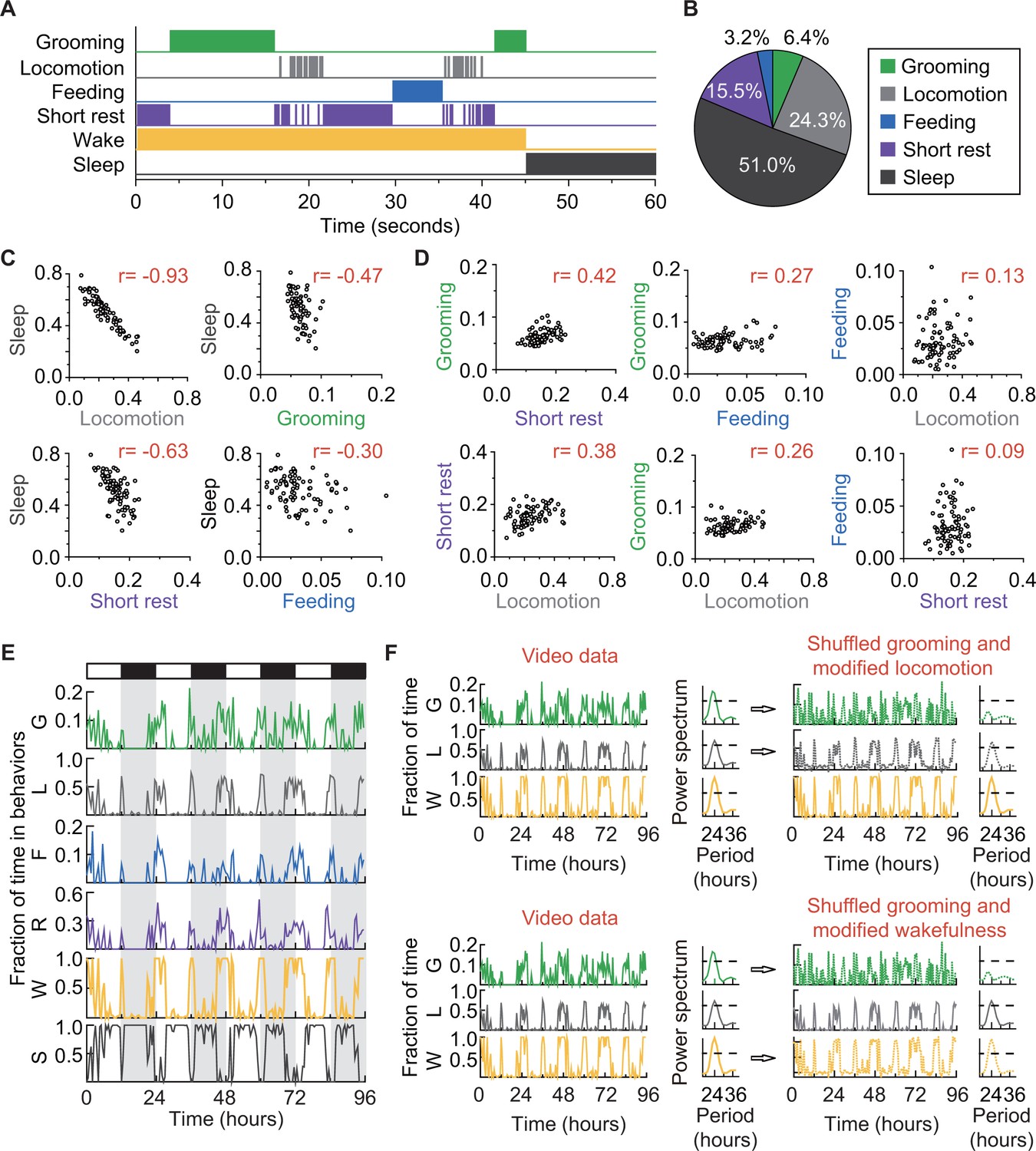
(A) Ethogram of grooming (green), locomotion (gray), feeding (blue), short rest (purple), and sleep (dark gray) performed by an *iso31+* fly in 60 s (300 frames). Individual events of these four behaviors are mutually exclusive and together constitute wake (yellow-orange), which is complementary to sleep (dark gray). (B) Average fraction of time flies spent in each behavior. N = 83 *iso31+* flies. (C) (D) Correlation between pairs of behaviors. There is strong negative correlation between sleep and locomotion (r = −0.93) and between sleep and short rest (r = −0.63). Interestingly, time spent in grooming does not show strong correlation with any of the other four behaviors. N = 83 *iso31+* flies. r is the Pearson product-moment correlation coefficient. (E) Temporal patterns of behaviors of a single *iso31+* fly during 4 days in LD cycles. Behaviors shown here are, grooming (G), locomotion (L), feeding (F), short rest (R), wake (W), and sleep (S). Level of activity is shown in terms of fraction of time spent in each behavior. Fraction is calculated every 30 min. White/black horizontal bars indicate light/dark environmental conditions, respectively. (F) Rhythmicity in grooming, locomotion and wake in an example fly. In LD condition, fraction of time spent in these behaviors are plotted on left. In power spectra on right of time series of behaviors (horizontal dash line denotes threshold power for p=0.05), temporal patterns of the three behaviors all show significant circadian rhythmicity. In right top, spectra of randomized grooming show no rhythmicity, while modified locomotion is still rhythmic. Similarly, in time series on right bottom, with the same randomized grooming, wake remains rhythmic while grooming, as one component from it, is arrhythmic. In time series of behaviors, activity is binned every 30 min.

https://doi.org/10.7554/eLife.34497.014

Figure 4—source data 1 Source data for Figure 4.: https://doi.org/10.7554/eLife.34497.018
Download elife-34497-fig4-data1-v2.xlsx
Figure 4—source data 2 Source data for Figure 4—figure supplement 1.: https://doi.org/10.7554/eLife.34497.019
Download elife-34497-fig4-data2-v2.xlsx
Figure 4—source data 3 Source data for Figure 4—figure supplement 2.: https://doi.org/10.7554/eLife.34497.020
Download elife-34497-fig4-data3-v2.xlsx

Figure 4—figure supplement 1

Download asset Open asset

Relationships among fly grooming, locomotion, feeding, short rest, and sleep.

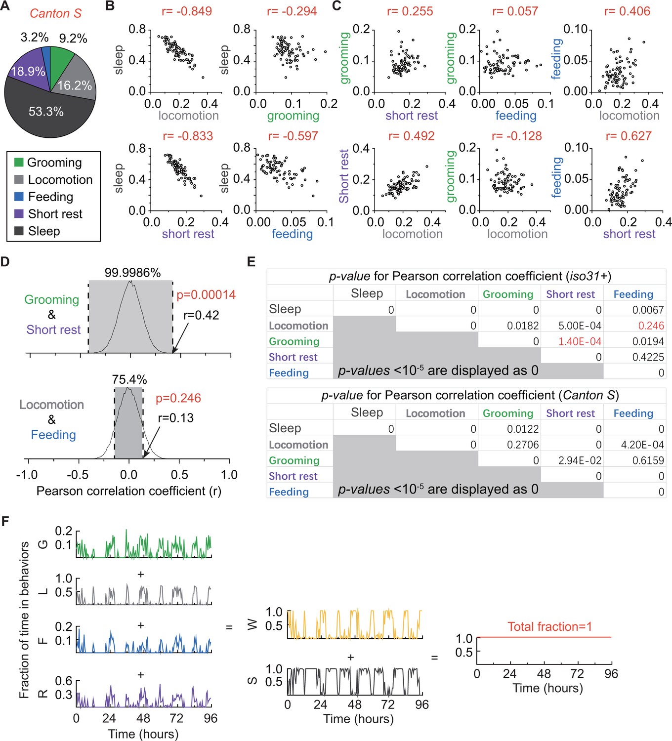
(A) Average fraction of time flies spent in grooming (green), locomotion (gray), feeding (blue), short rest (purple), and sleep (dark gray). N = 76 *Canton S* flies. (B) (C) Correlation between behaviors. Sleep shows different levels of negative correlation to locomotion (r = −0.849), short rest (r = −0.833) and feeding (−0.597). In addition, there is positive correlation between locomotion and short rest (r = 0.627). Interestingly, time spent in grooming does not show strong correlation with any of the other four behaviors. This suggests independent regulation of grooming behavior. N = 76 *Canton S* flies. (D) Example empirical probability distributions of random paired r values between grooming and short rest (top) and between locomotion and feeding (bottom) in iso31+ flies. p-Values of Pearson coefficient r were calculated based on two-tailed test of such distributions. (E) p-Values of all Pearson correlation coefficients r in Figure 4C,D (top table) and Figure 4—figure supplement 1B,C (bottom table). p-Values in red are from examples in (D). p<10⁻⁵ is displayed as 0 in these tables. (F) Example of binned data (reproduced from Figure 4E) showing fraction of time in different behaviors. In this representation, behaviors are not mutually exclusive and each behavior is free to assume any value between 0 and 1 (inclusive) such that wake time +sleep time=1 for every bin. Grooming: G, Locomotion: L, Feeding: F, Short rest: R, Wake; W, Sleep: S.

https://doi.org/10.7554/eLife.34497.015

Figure 4—figure supplement 2

Download asset Open asset

Temporal relationships between grooming and locomotion.

(A) Position within the tube (top row), locomotion (middle) and grooming (bottom) of a single *iso31+* fly during one day in LD. Locomotion and grooming are shown in terms of fraction of time spent in 5 min bins. White/black bars indicate light/dark environmental conditions, respectively. (B) Probability density of the intervals between grooming events (green) and between locomotion events (gray). Probability distributions were constructed from ~33,000 intervals between grooming events and ~73,000 intervals between locomotion events detected in 83 *iso31+* flies. (C) Longest intervals between grooming events (green) and between locomotion events (gray). Each point represents an individual fly recorded for a day. N = 83 *iso31+* flies, p=1.2 $\times$ 10⁻¹⁹. (D) Probability density of the duration of grooming events (green) and locomotion events (gray). Probability distributions were constructed from ~33,000 grooming events and ~73,000 locomotion events detected in 83 *iso31+* flies. (E) Longest duration of grooming (green) and locomotion events (gray). Each point represents an individual fly recorded for a day. N = 83 *iso31+* flies, p=3.6 $\times$ 10⁻⁸. (F) (G) Example fits (red) of temporal patterns of grooming activity (green) and locomotion activity (gray) of an individual fly during 3 days in LD environment. Horizontal white/black bars represent alternating light/dark conditions. (H) Sketch of the mathematical model that uses four exponential terms to describe temporal patterns of a fly activity. Parameters $b_{M D}$ , $b_{E R}$ , $b_{E D}$ , $b_{M R}$ , TM and TE (see Figure 4—figure supplement 3) are marked in the plot. (**I–N**) Comparison of parameter values yielded by fits to locomotion and grooming data. Each circle represents an individual fly (N = 9). Data from same fly are connected by a solid line. (O) Average amount time spent in grooming (green), visiting food (blue) and locomotion (gray) during two days in LD. Each behavior time series is normalized by its maximum to allow for easy comparison of their relative phases. In wild-type flies (top panel), burst in visiting food happens ~1 hr after the morning peak in locomotion. Onset of evening peaks in grooming usually occurs earlier than the peak in locomotion. Time difference between peak in feeding and grooming is considered as the time delay of grooming peak after feeding, as indicated by red arrows. N = 50 *iso31+* flies. (P) The time difference in onset of bursts in grooming and locomotion (gray), grooming and feeding (blue), in LD conditions. Discreteness in time differences is a consequence of binning the time-series in 30 min. N = 50 *iso31+* flies.

https://doi.org/10.7554/eLife.34497.016

Figure 4—figure supplement 3

Download asset Open asset

Mathematical description of temporal changes in grooming and locomotion patterns.

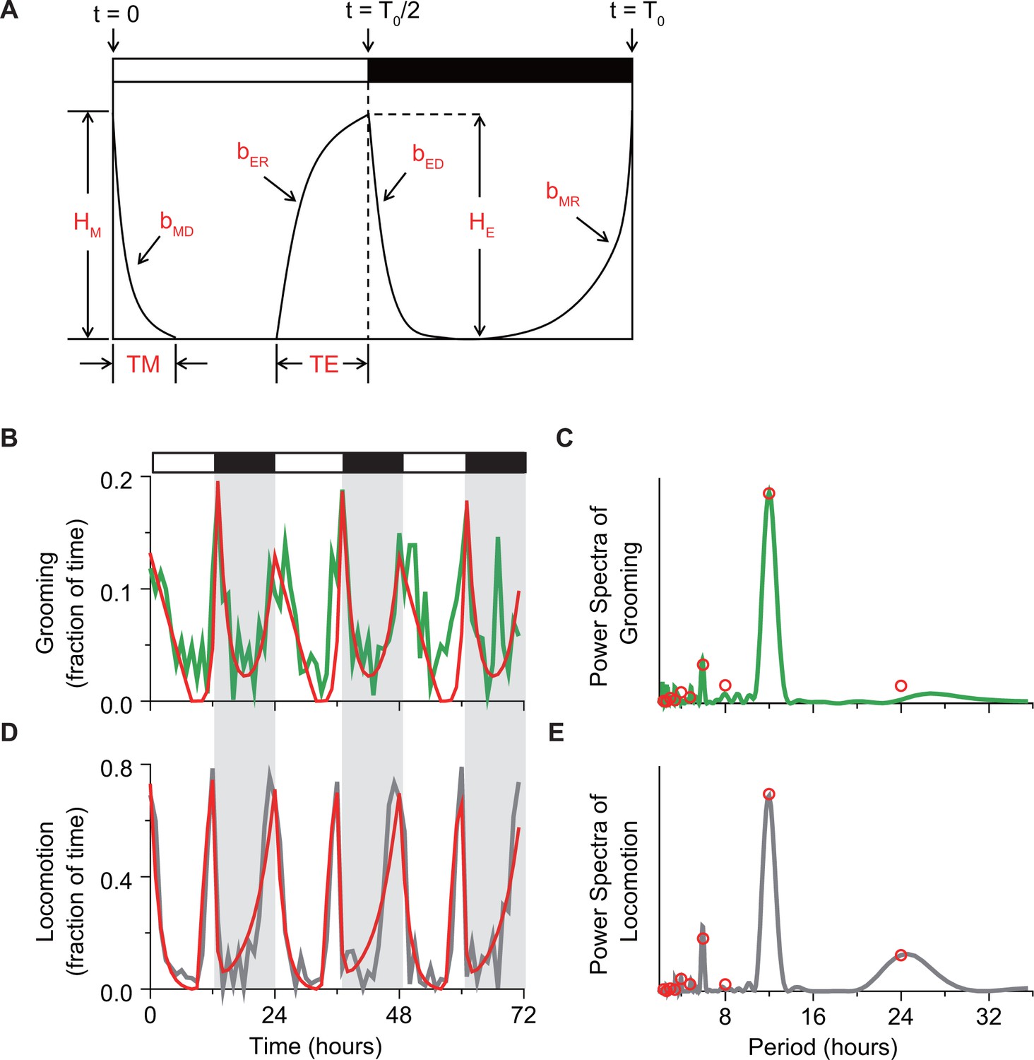
(A) Sketch of the mathematical model that uses four exponential terms to describe temporal patterns of a fly activity. Horizontal white/black bars represent alternating light/dark conditions. (B, C) Example fits (red) of (B) temporal pattern and (C) power spectrum of grooming activity (green) of an individual fly during 3 days in LD environment. The activity data are binned in 1 hr for visual clarity. (D, E) Example fits (red) of (D) temporal pattern and (E) power spectrum of locomotion activity (gray) of an individual fly during 3 days in LD environment. The activity data are binned in 1 hr for visual clarity. To quantitatively compare the temporal patterns of grooming and locomotion (Figure 4—figure supplement 2), we applied a previously developed mathematical method that allows quantification of the main features in fly locomotion pattern. (Lazopulo and Syed, 2016). The quantification is achieved by fitting activity data with a model that consists of four exponential terms:
$F (t) = {\begin{matrix} H_{M} \frac{e^{b_{M D} T_{M}} - e^{b_{M D} t}}{e^{b_{M D} T_{M}} - 1}, & 0 < t < T_{M} \\ H_{M} \frac{e^{b_{M R} (t - T_{M})} - 1}{e^{b_{M R} (T_{o} - T_{M})}}, & T_{M} < t < T_{0} \\ H_{E} \frac{1 - e^{- b_{E R (t - \frac{T_{o}}{2} - T_{E})}}}{1 - e^{- b_{E R} T_{E}}}, & \frac{T_{0}}{2} - T_{E} < t < \frac{T_{0}}{2} \\ H_{E} e^{- b_{E D t - \frac{T_{o}}{2}}}, & \frac{T_{0}}{2} < t < T_{0} \end{matrix}$
The model has nine independent parameters that describe activity pattern. Parameters $b_{M D}$ , $b_{M R}$ , $b_{E D}$ , $b_{E R}$ define rates of morning decay (MD), morning rise (MR), evening decay (ED) and evening rise (ER), respectively. Parameter T₀ defines circadian period, $T_{M}$ and $T_{E}$ define widths of M and E peaks, and $H_{M}$ and $H_{E}$ define heights of M and E peaks, as shown in sketch in panel (A). The white and black horizontal bars represent lights-on and -off phases of the external light-dark cycle. Values of the parameters are obtained from the activity data in a few steps. First, the circadian period is estimated from the power spectrum of activity data. Then, preliminary parameter values are estimated by fitting the locomotion recording with the function $F (t)$ . These values serve as initial guess for fitting the data power spectrum with an analytical expression derived by calculating the Fourier transform of $F (t)$ :
$\tilde{F} (T_{n}) = \frac{1}{T_{0}} \int_{0}^{T_{0}} F (t) e^{\frac{i 2 π n}{T_{0}}} d t,$
where $T_{n}$ = $T_{0} / n$ , with $n = 1, 2, 3 \dots$ and $T_{0}$ is the circadian period. By using the spectral fit, we extract model parameters without filtering or binning. Fitting of the power spectrum produces final values for the model parameters, which are then used to construct the final form of $F (t)$ , our model of fly activity rhythms. Examples of fits of grooming and locomotion activities and their respective power spectra are provided in panels (B–E). Parameter values and least squares fitting errors of fitting locomotion and grooming spectrum of nine representative individual flies are shown in Table 1 and Table 2. Here the fitting error is calculated from.
$Error = \frac{\sum_{i} (P_{f i t}^{i} - P_{a c t u a l}^{i})}{\sum_{i} (P_{f i t}^{i} - P_{r a n d o m}^{i})}$
where $P_{a c t u a l}^{i}$ and $P_{f i t}^{i}$ are the actual spectral power and fitted spectral power at the $i$ th spectral frequency, respectively. $P_{r a n d o m}^{i}$ is the averaged spectral power from randomly shuffled data at the $i$ th frequency. To get $P_{r a n d o m}^{i}$ , we first randomly shuffle activity data 100 times and compute power spectrum for each of them. Then $P_{r a n d o m}^{i}$ is the average of 100 individual spectral power at the ith frequency.

https://doi.org/10.7554/eLife.34497.017

Figure 5 with 3 supplements

Download asset Open asset

Grooming is under control of the circadian clock.

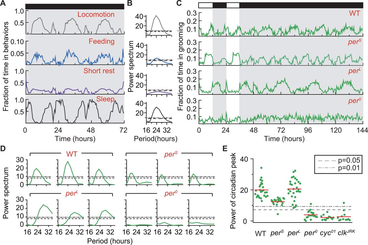
(A) Average temporal patterns (fraction of time spent in 30 min bins) of locomotion, feeding, short rest and sleep of eight representative *iso31+* flies during 3 days in constant darkness (DD). Black horizontal bar represents lights-off condition. (B) Power spectra of behaviors in panel (A). Except for short rest, temporal patterns of the other three behaviors show significant circadian rhythmicity. Horizontal dash line and dash dot line denote threshold powers for p=0.05 and p=0.01, respectively. (C) Grooming activity (in 30 min bins) of wild-type and clock mutants during 2 days in LD cycle followed by four days in DD cycle. Grooming traces are population averages. In DD, wild-type (WT, *iso31+*) grooming continues to show 24 hr rhythms. In comparison, grooming in ${p e r}^{S}$ or ${p e r}^{L}$ flies show shorter or longer rhythms, respectively. For ${p e r}^{0}$ flies, grooming is arrhythmic in DD. N = 8 WT, 8 ${p e r}^{S}$ , 8 ${p e r}^{L}$ , and 8 ${p e r}^{0}$ representative flies. (D) Example power spectra showing circadian rhythmicity in grooming patterns of three individual wild-type, ${p e r}^{S}$ , ${p e r}^{L}$ and ${p e r}^{0}$ flies. Spectra are normalized to variance of activity (in 30 min bins). Dash lines and dash dot lines represent threshold power at p=0.05 and p=0.01, respectively. More examples of individual power spectra are provided in Figure 5—figure supplement 1. (E) Spectral powers of circadian peaks of individual wild-type and circadian mutants. N = 29 control, 20 ${p e r}^{S}$ , 29 ${p e r}^{L}$ , 20 ${p e r}^{0}$ , 13 ${c y c}^{01}$ and 11 ${c l k}^{J R K}$ .

https://doi.org/10.7554/eLife.34497.023

Figure 5—source data 1 Source data for Figure 5.: https://doi.org/10.7554/eLife.34497.027
Download elife-34497-fig5-data1-v2.xlsx
Figure 5—source data 2 Source data for Figure 5—figure supplement 1.: https://doi.org/10.7554/eLife.34497.028
Download elife-34497-fig5-data2-v2.xlsx
Figure 5—source data 3 Source data for Figure 5—figure supplement 3.: https://doi.org/10.7554/eLife.34497.029
Download elife-34497-fig5-data3-v2.xlsx
Figure 5—source data 4 Source data for Figure 5—figure supplement 2.: https://doi.org/10.7554/eLife.34497.030
Download elife-34497-fig5-data4-v2.xlsx

Figure 5—figure supplement 1

Download asset Open asset

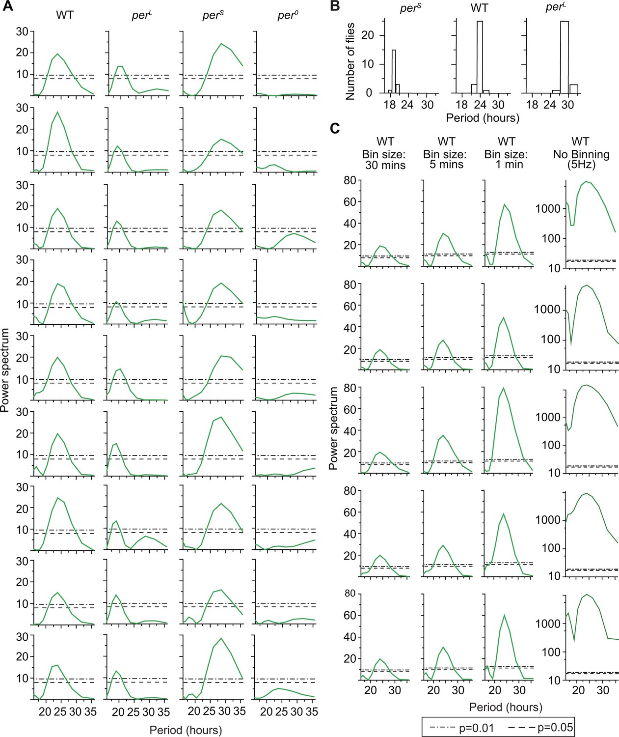
(A) Example Lomb-Scargle periodograms of grooming activity of individual *per* mutants and their background control (WT).

Spectra are normalized by dividing by variance of individual grooming activity binned in 30 min. Dash lines and dash dot lines represent threshold power at p=0.05 and p=0.01 respectively. Spectra of *per^S*, *per^L*, and wt grooming show significant rhythmicities in accordance with their known effects on the pace of the clock. Grooming of *per⁰* flies (fourth column from left) are arrhythmic according to the individual spectral analyses. (B) Periods of significant rhythmicity (at p=0.01 level) in grooming of individual wt, *per^S* and *per^L* flies. Different bin sizes of periods is a result of evenly sampled frequencies in spectral analysis. N = 29 wt, 19 ${p e r}^{S}$ , and 29 ${p e r}^{L}$ . (C) To test the effect of binning on rhythmicity, we took grooming data of individual flies recorded at 5 Hz, binned them in 30 min, 5 min and 1 min and ran Lomb-Scargle periodogram analysis on these time-series. Examples of five individual spectra of each bin size are shown here. In general, smaller bin size increases the separation between statistical cut-off power (p value, horizontal lines) and peak power because of their differential dependence on the number of data points in a time-series (see Materials and methods).

https://doi.org/10.7554/eLife.34497.024

Figure 5—figure supplement 2

Download asset Open asset

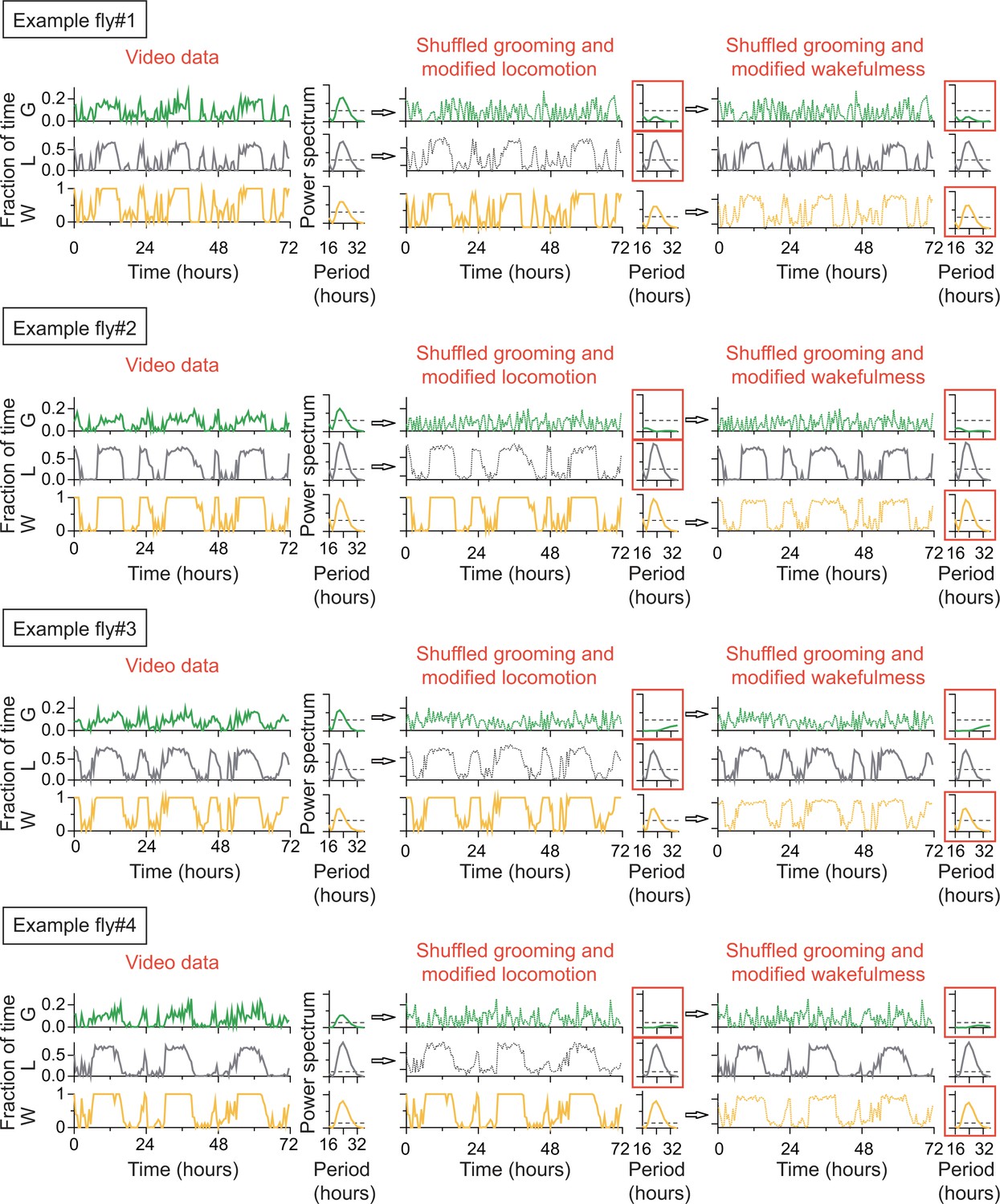
Rhythmicity in grooming patterns need not be a direct result of rhythmicity in locomotion or sleep-wake cycles.

For each of the four example flies, raw data of the fraction of time spent in locomotion, grooming and wake behaviors are plotted on left column. Their power spectra (adjacent plots) show significant circadian rhythmicity at p=0.05 level (horizontal dashed line). If raw grooming data are randomly shuffled and locomotion is modified accordingly so that wake is unchanged (middle column), power spectrum of randomized grooming shows no rhythmicity, while modified locomotion is still rhythmic. If instead wake data are modified when grooming are randomized (right column) so that locomotion is unchanged, then grooming again loses rhythmicity while wake remains rhythmic. Time series in the four examples were taken in constant darkness (DD) and binned in 30 min and Lomb-Scargle periodogram were calculated from the binned data.

https://doi.org/10.7554/eLife.34497.025

Figure 5—figure supplement 3

Download asset Open asset

(A) Locomotion (in 30 min bins) of wild-type (*iso31+*) and clock mutants during two days in LD cycle followed by four days in DD cycle.

Locomotion traces are population averages. In DD, wt locomotor activity continues to show 24 hr rhythms. In comparison, locomotion in ${p e r}^{S}$ or ${p e r}^{L}$ flies show shorter or longer rhythms, respectively. For ${p e r}^{0}$ flies, locomotion appears arrhythmic in DD. N = 8 WT, 8 ${p e r}^{S}$ , 8 ${p e r}^{L}$ , 8 ${p e r}^{0}$ flies. (B) Temporal patterns of population averaged grooming of two additional arrhythmic strains during 3 days in DD conditions. Top panel shows *cyc⁰¹* (N = 13) and bottom shows *clk^JRK* (N = 11). Data are binned in 30 min. (C) (D) Average of spectra of individual *cyc⁰¹* (panel C left, N = 13) and *clk^JRK* (panel D, left, N = 11) grooming. Dash lines and dash dot lines represent threshold power at p=0.05 and p=0.01, respectively. Example spectra of individual *cyc⁰¹* (C) and *clk^JRK* (D) flies show power over the circadian range are well below the p=0.05 level.

https://doi.org/10.7554/eLife.34497.026

Figure 6 with 1 supplement

Download asset Open asset

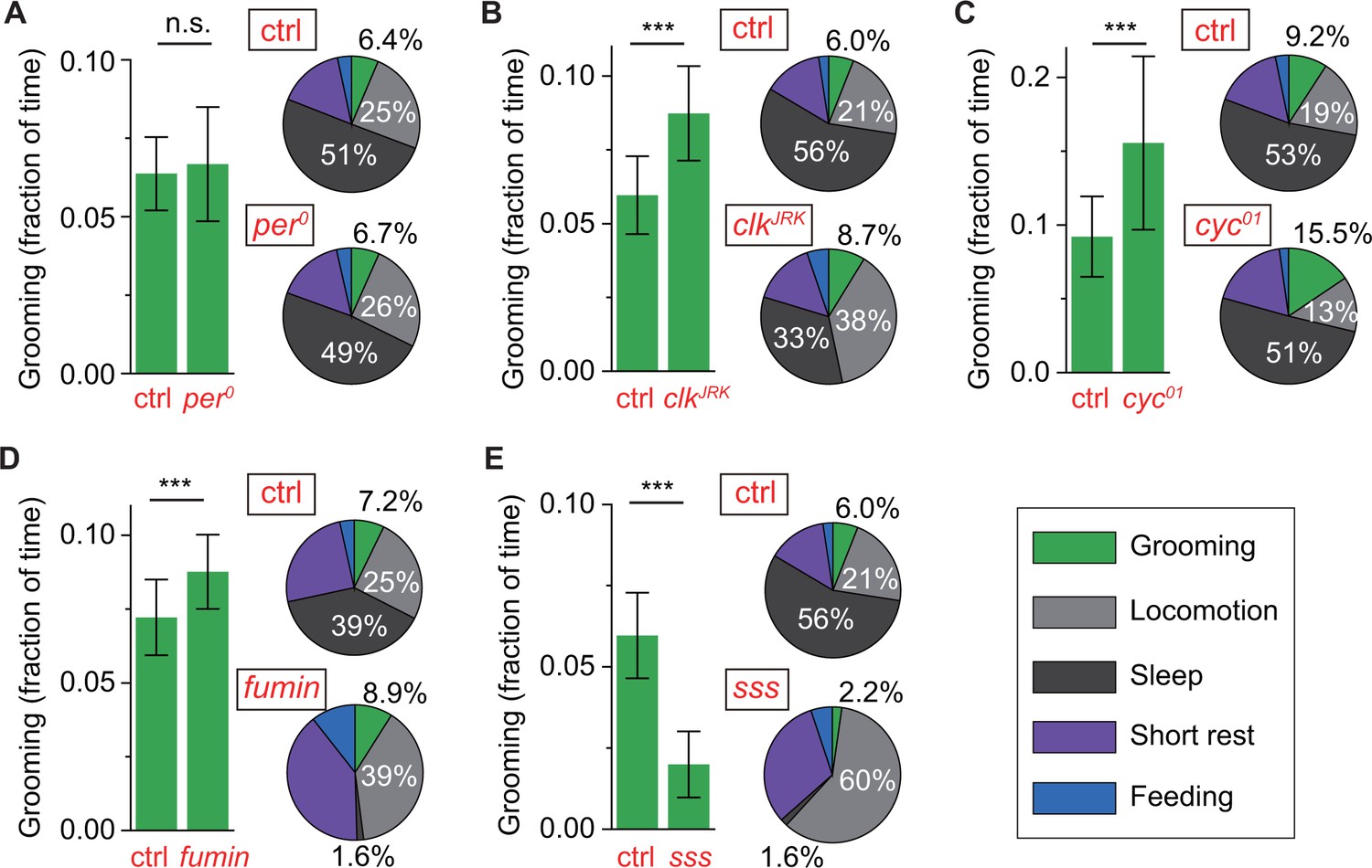
Control of grooming duration is independent of circadian rhythmicity.

In each panel, bar plots on left show average fractional time spent in grooming in mutant and control flies. Pie charts on right present average fractional time spent in grooming (green), locomotion (gray), sleep (dark gray), short rest (purple) and feeding (blue). Here, numerical values for fractional time spent in behavior are indicated only for grooming, locomotion and sleep with additional details in Figure 6—figure supplement 1A. Although loss of a functional clock does not affect grooming amount (A), mutations in *clock* (B) and *cycle* (C) genes lead to robust increases in the time flies spend grooming. Additional time for grooming can come from reduction in sleep (B) or reduction in locomotion (C). Reduction in sleep, however, does not always entail similar changes in grooming since sleep mutants *fumin* (D) and *sleepless* (E) show divergent alterations in grooming durations. N = 83 control, 53 ${p e r}^{0}$ , p=0.28. N = 76 control, 18 ${c y c}^{01}$ , p=2.7 $\times$ 10⁻⁴. N = 28 control, 25 ${c l k}^{J R K}$ , p=7.8 $\times$ 10⁻⁹. N = 17 control, 23 *fumin*, p=0.003. N = 28 control, 17 *sss, p*=1.3 $\times$ 10⁻¹⁰.

https://doi.org/10.7554/eLife.34497.031

Figure 6—source data 1 Source data for Figure 6.: https://doi.org/10.7554/eLife.34497.033
Download elife-34497-fig6-data1-v2.xlsx
Figure 6—source data 2 Source data for Figure 6—figure supplement 1.: https://doi.org/10.7554/eLife.34497.034
Download elife-34497-fig6-data2-v2.xlsx

Figure 6—figure supplement 1

Download asset Open asset

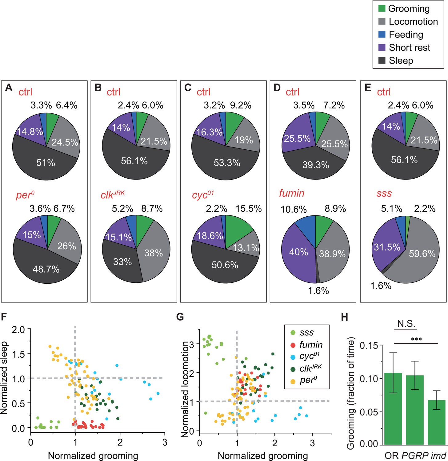
Changes in grooming due to mutations in clock, sleep or immune genes.

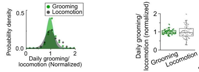
(A)-(E) Average fraction of time flies spent in grooming (green), locomotion (gray), sleep (dark gray), short rest (purple) and feeding (blue). N = 53 ${p e r}^{0}$ and 83 control, 18 ${c y c}^{01}$ and 76 control, 25 ${c l k}^{J R K}$ and 28 control, 23 *fumin* and 17 control, 17 *sss* and 28 control. (F) Correlation between normalized sleep and grooming in *sss, fumin*, *cyc⁰¹*, and *clk^JRK* flies. (G) Correlation between normalized locomotion and grooming in *sss, fumin*, *cyc⁰¹* and *clk^JRK* flies. (F)-(G) For the mutants, the fraction of time spent in behaviors are normalized by dividing by the average fraction of time in that behavior by their respective control flies. N = 17 *sss*, 23 *fumin,* 18 *cyc⁰¹*, 25 *clk^JRK*, and 53 ${p e r}^{0}$ . (H) Population-averaged fractional time spent in grooming. Grooming in *imd* flies are significantly less than control flies (p<0.001), while *PGRP-SA*^seml does not significantly affect the time spent in grooming. This suggests that *Drosophila* grooming relies on a working immune system. The decrease in *imd* flies further suggests that this impact may be independent of the Toll pathway. N = 56 OR, 47 *PGRP-SA*^seml, 45 *imd*.

https://doi.org/10.7554/eLife.34497.032

Author response image 1

Download asset Open asset

Author response image 2

Download asset Open asset

Videos

Video 1

Download asset

posterframe for video — Sample raw experimental video
https://doi.org/10.7554/eLife.34497.004

Video 2

Download asset

Video 3

Download asset

Video 4

Download asset

Tables

Table 1

Parameter values and fitting errors from fitting grooming time-series

https://doi.org/10.7554/eLife.34497.021

Fly #	*b_MD*	*b_MR*	*b_ER*	*b_ED*	T₀	*T_M*	*T_E*	*H_M*	*H_E*	Error
1	0.000	0.007	−0.024	0.010	23.9	6.0	3.0	294	442	0.0115
2	0.008	0.008	−0.055	0.014	23.9	3.0	5.0	280	344	0.0894
3	−0.008	0.005	−0.070	0.027	24	4.0	3.0	295	811	0.0674
4	−0.019	0.003	−0.035	0.046	24	4.0	3.0	204	540	0.0674
5	0.002	0.007	−0.042	0.019	24	4.0	2.0	262	1155	0.0541
6	−0.013	0.005	0.009	0.026	24	3.0	3.0	171	317	0.0115
7	0.026	0.003	−0.018	0.006	24.3	4.0	3.0	210	436	0.076
8	0.110	0.008	−0.012	0.015	23.9	2.0	5.0	158	344	0.0057
9	−0.015	0.003	−0.001	0.098	23.9	3.0	4.0	267	475	0.0175

Table 2

Parameter values and fitting errors from fitting locomotion time-series

https://doi.org/10.7554/eLife.34497.022

Fly #	*b_MD*	*b_MR*	*b_ER*	*b_ED*	T₀	*T_M*	*T_E*	*H_M*	*H_E*	Error
1	−0.001	0.004	0.004	0.033	24.0	6.0	2.0	1631	1675	0.01
2	−0.005	0.073	−0.069	0.028	24.1	2.0	2.0	825	1434	0.0037
3	−0.013	0.063	0.020	0.002	23.9	2.9	1.9	4162	1208	0.0469
4	−0.010	0.020	0.022	0.001	23.7	3.0	2.0	3355	1388	0.001
5	0.055	0.060	−0.338	0.007	24	3.0	3.0	741	1948	0.0056
6	0.009	0.015	−0.054	0.028	23.6	3.0	3.0	1509	1369	0.1029
7	0.001	0.028	−0.022	0.023	24	2.0	3.0	1535	1010	0.0072
8	−0.015	0.008	−0.007	0.032	23.9	3.0	2.0	1504	2308	0.007
9	0.014	0.020	−0.028	0.016	23.9	3.0	3.0	1519	2004	0.0007

Key resources table

Reagent type (species) or resource	Designation	Source or reference	Identifiers	Additional information
Strain, strain background (Drosophila melanogaster, male)	sss^p1	DOI: 10.1126/science.1155942		on iso31 background
Strain, strain background (D. melanogaster, male)	iso31	DOI: 10.1126/science.1155942
Strain, strain background (D. melanogaster, male)	fumin	DOI: 10.1523/JNEUROSCI.2048-05.2005		on w¹¹¹⁸ background
Strain, strain background (D. melanogaster, male)	w¹¹¹⁸	Bloomington Drosophila Stock Center	BDSC: 3605
Strain, strain background (D. melanogaster, male)	Canton S	Bloomington Drosophila Stock Center	BDSC: 64349
Strain, strain background (D. melanogaster, male)	clk^JRK	this paper		backcrossed for five generations to iso31
Strain, strain background (D. melanogaster, male)	per⁰	this paper		backcrossed for five generations to iso31⁺
Strain, strain background (D. melanogaster, male)	per^S	this paper		backcrossed for six generations to iso31⁺
Strain, strain background (D. melanogaster, male)	per^L	this paper		backcrossed for six generations to iso31⁺
Strain, strain background (D. melanogaster, male)	cyc⁰¹	other		on Canton S background, gifts from William Ja
Strain, strain background (D. melanogaster, male)	iso31⁺	other		gifts from Michael Young