Figures and data in A spike sorting toolbox for up to thousands of electrodes validated with ground truth recordings in vitro and in vivo

Figures
Tables
Additional files

4 figures, 1 table and 1 additional file

Figures

Figure 1 with 1 supplement

Download asset Open asset

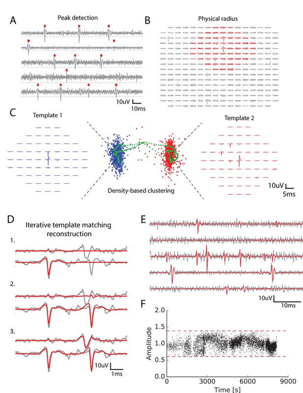
Main steps of the spike sorting algorithm.

(A) Five randomly chosen electrodes, each of them with its own detection threshold (dash dotted line). Detected spikes, as threshold crossings, are indicated with red markers (B) Example of a spike in the raw data. Red: electrodes that can be affected by the spike, that is the ones close enough to the electrode where the voltage peak is the highest; gray: other electrodes that should not be affected. (C) Example of two clusters (red and blue)with associated templates. Green points show possible combinations of two overlapping spikes from the two cells for various time delays. (D) Graphical illustration of the template matching for in vitro data (see Materials and methods). Every line is a electrode. Grey: real data. Red: sum of the templates added by the template matching algorithm; top to bottom: successive steps of the template matching algorithm. E. Final result of the template matching. Same legend as (D, F) Examples of the fitted amplitudes for the first component of a given template as a function of time. Each dot correspond to a spike time at which this particular template was fitted to the data. Dashed dotted lines represent the amplitude thresholds (see Materials and methods).

https://doi.org/10.7554/eLife.34518.002

Figure 1—figure supplement 1

Download asset Open asset

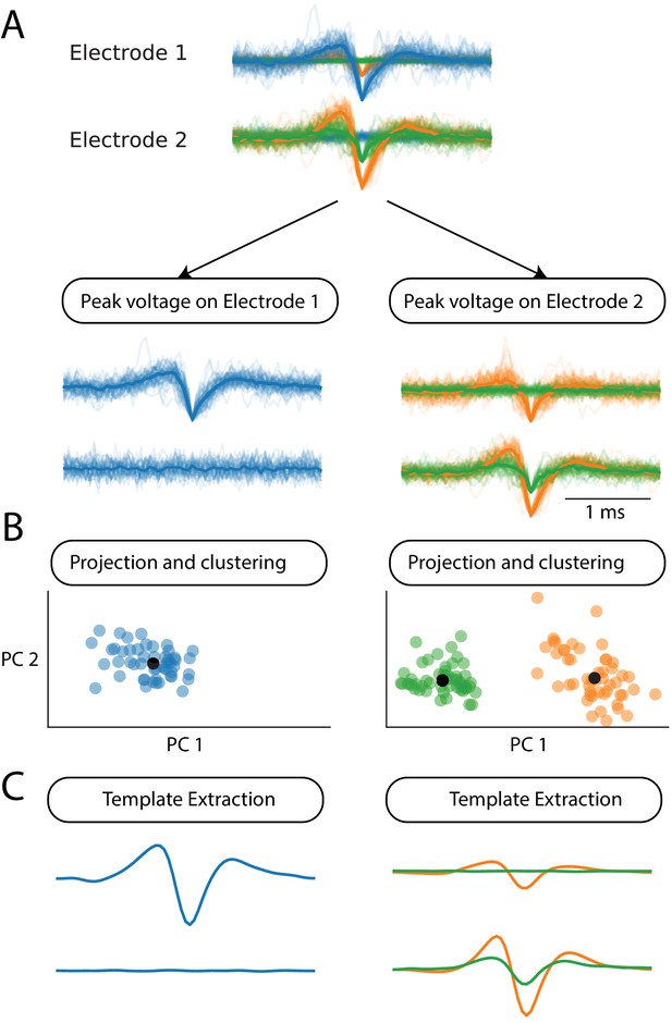
Schematic of the parallel clustering of the spikes, in a toy example with two electrodes.

(A) Pre-clustering step. The different snippets are sorted according to the electrode where they peak. This divides a set of snippets in $N_{elec}$ groups. Each of these groups is then processed independently. (B) Each group of snippets is projected in a low-dimension space, where clustering is performed using a density-based approach (see text and Materials and methods). (C) A template is extracted from each cluster and used for the template matching step.

https://doi.org/10.7554/eLife.34518.003

Figure 2

Download asset Open asset

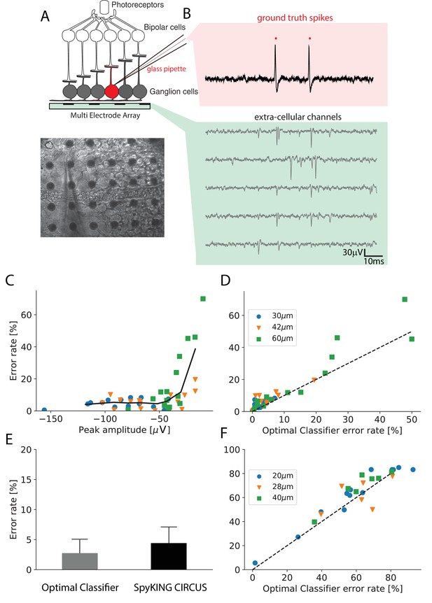
Performance of the algorithm on ground truth datasets.

(A) Top: Schematic of the experimental protocol in vitro. A neuron close to the multielectrode array (MEA) recording is recorded in loose patch. Bottom: Image of the patch electrode on top of a 252 electrodes MEA, recording a ganglion cell. (B) Top, pink box: loose patch recording showing the spikes of the recorded neuron. Bottom, green box: Extra-cellular recordings next to the loose patched soma. Each line is a different electrode (C) Error rate of the algorithm as function of the largest peak amplitude of the ground-truth neuron, recorded extracellularly in vitro. (D) Comparison between the error rates produced by the algorithm on different ground truth datasets and the error rates of nonlinear classifiers (Best Ellipsoidal Error Rate) trained to detect the spikes for in vitro data (Spampinato et al., 2018). (E) Comparison of average performance for all neurons detected by the Optimal Classifier with an error less than 10% (n = 37). F. Same as D. but for in vivo data (Neto et al., 2016) (see Materials and methods).

https://doi.org/10.7554/eLife.34518.004

Figure 3

Download asset Open asset

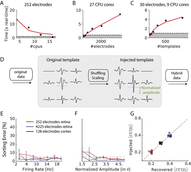
Scaling to thousands of electrodes.

(A) Execution time as function of the number of processors for a 90 min dataset in vitro with 252 electrodes, expressed as a real-time ratio, that is the number of hours necessary to process one hour of data. (B) Execution time as function of the number of electrodes for a 30 min dataset recorded in vitro with 4225 electrodes. (C) Execution time as function of the number of templates for a 10-min synthetic dataset with 30 electrodes. (D) Creation of ‘hybrid’ datasets: chosen templates are injected elsewhere in the data as new templates. Dashed-dotted lines shows the detection threshold on the main electrode for a given template, and normalized amplitude is expressed relative to this threshold (see Materials and methods). (E) Mean error rate as function of the firing rate of injected templates, in various datasets. Errors bars show standard error over eight templates (F) Error rate as function of the normalized amplitude of injected templates, in various datasets. Errors bars show standard error over nine different templates (G) Injected and recovered cross-correlation value between pairs of neurons for five templates injected at 10 Hz, with a normalized amplitude of 2 (see Materials and methods).

https://doi.org/10.7554/eLife.34518.005

Figure 4

Download asset Open asset

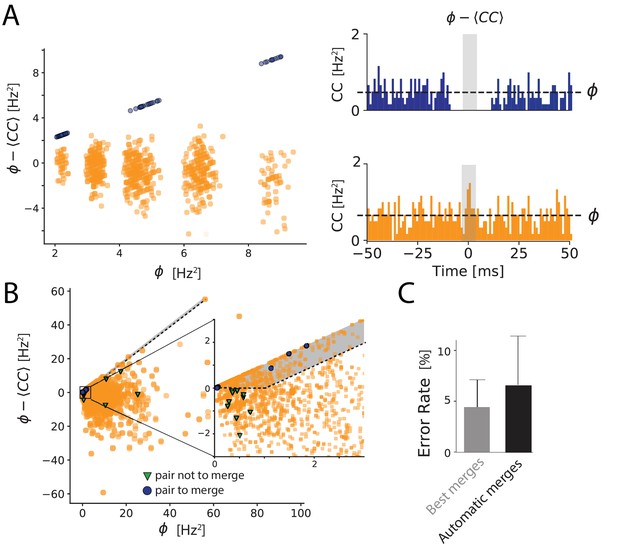
Automated merging.

(A) Dip estimation (y-axis) compared to the geometrical mean of the firing rate (x-axis) for all pairs of units and artificially generated and split spike trains (see Materials and methods). Blue: pairs of templates originating from thesame neuron that have to be merged. Orange: pairs of templates corresponding to different cells. Panels on the right: for two chosen pairs, one that needs to be merged (in blue, top panel) and one should not be merged (orange, bottom panel) the full cross-correlogram and the geometrical mean of the firing rate (dashed line). The average correlation is estimated in the temporal window defined by the gray area. (B) Same as A, for a ground truth dataset. Blue points: points that need to be merged. Green points: pairs that should not be merged. Orange points: pairs where our ground truth data does not allow us telling if the pair should be merged or not. The gray area corresponds to the region where pairs are merged by the algorithm. Inset: zoom on one region of the graph. (C) Average error rate in the case where the decision of merging units was guided by the ground truth data (left) against the automated strategy designed here (right).

https://doi.org/10.7554/eLife.34518.006

Tables

Table 1

Table of all the variables and notations found in the algorithm.

https://doi.org/10.7554/eLife.34518.007

Variable	Explanation	Default value
	Generic notations
$N_{elec}$	Number of electrodes
$p_{k}$	Physical position of electrode $k$ [ $μ$ m]
$G_{k}$	Ensemble of nearby electrodes for electrode $k$ [ $μ$ m]
$N_{neigh}^{k}$	Cardinal of $G_{k}$
$θ_{k}$	Spike detection threshold for electrode $k$ [ $μ$ V]
$s (t)$	Raw data [ $μ$ V]
$w_{j} (t)$	First component of the template for neuron $j$ [ $μ$ V]
$v_{j} (t)$	Second component of the template for neuron $j$ [ $μ$ V]
$f_{rate}$	Sampling frequency of the signal [Hz]
	Preprocessing of the data
$f_{cut}$	Cutoff frequency for butterworth filtering	100 Hz
$N_{t}$	Temporal width for the templates	5 ms
$r_{max}$	Spatial radius for the templates	250 $μ$ m
$λ$	Gain for threshold detection for channel $k$ ( $θ_{k}$ )	6
$N_{p}$	Number of waveforms collected per electrode	10000
$N_{PCA}$	Number PCA features kept to describe a waveform	5
	Clustering and template estimation
$x_{1, .. l}^{k}$	$l$ spikes peaking on electrode $k$ and projected after PCA
$ρ_{l}^{k}$	Density around $x_{l}^{k}$
$δ_{l}^{k}$	Minimal distance from $x_{l}^{k}$ to spikes with higher densities
$N_{spikes}$	Number of spikes collected per electrode for clustering	10000
$N_{{PCA}_{2}}$	Number of PCA features kept to describe a spike	5
$S$	Number of neighbors for density estimation	100
$N_{max}^{clusters}$	Maximal number of clusters per electrode	10
$ζ$	Normalized distance between pairs of clusters
$σ_{similar}$	Threshold for merging clusters on the same electrode	3
$α_{m}$	Centroid of the cluster $m$
$γ_{m}$	Dispersion around the centroid $α_{m}$
$η$	Minimal size of a cluster (in percent of $N_{spikes}$ )	0.005
$[a_{min}, a_{max}]$	Amplitudes allowed during fitting for a given template
	Dictionary cleaning
$C C_{max} (m, n)$	Max over time for the Cross-correlation between $w_{m}$ and $w_{n}$
$c c_{similar}$	Threshold above which templates are considered as similar	0.975
	Template matching
$a_{i j}$	Product between $s (t)$ and $w_{j}$ (normalized) at time $t_{i}$
$b_{i j}$	Same as $a_{i j}$ but for the second component $v_{j}$
$n_{failures}$	Number of fitting attempts for a given spike time	3
	Automated merging
$c c_{merge}$	Similarity threshold to consider neurons as a putative pair	0.8
$r_{m, n} (t)$	Cross correlogram between spikes of unit $m$ and $n$
$ϕ (m, n)$	Geometrical mean of the firing rates for units $m$ and $n$ [Hz $^{2}$ ]
$ϕ_{merge}$	Maximal value for the dip in the cross correlogram at time 0	0.1 [Hz $^{2}$ ]

Additional files

Transparent reporting form: https://doi.org/10.7554/eLife.34518.008
Download elife-34518-transrepform-v2.pdf

Download links

A two-part list of links to download the article, or parts of the article, in various formats.

Downloads (link to download the article as PDF)

Open citations (links to open the citations from this article in various online reference manager services)

Mendeley

Cite this article (links to download the citations from this article in formats compatible with various reference manager tools)

Pierre Yger
Giulia LB Spampinato
Elric Esposito
Baptiste Lefebvre
Stéphane Deny
Christophe Gardella
Marcel Stimberg
Florian Jetter
Guenther Zeck
Serge Picaud
Jens Duebel
Olivier Marre

(2018)

A spike sorting toolbox for up to thousands of electrodes validated with ground truth recordings in vitro and in vivo

eLife 7:e34518.

https://doi.org/10.7554/eLife.34518

Share this article

Cite this article

Main steps of the spike sorting algorithm.

Schematic of the parallel clustering of the spikes, in a toy example with two electrodes.

Performance of the algorithm on ground truth datasets.

Scaling to thousands of electrodes.

Automated merging.

Table of all the variables and notations found in the algorithm.

Transparent reporting form

Downloads (link to download the article as PDF)

Open citations (links to open the citations from this article in various online reference manager services)

Cite this article (links to download the citations from this article in formats compatible with various reference manager tools)