Multi-scale mapping along the auditory hierarchy using high-resolution functional UltraSound in the awake ferret
- Laboratoire des Systèmes Perceptifs CNRS UMR 8248, École Normale Supérieure, PSL Research University, France
- Institut Langevin, ESPCI ParisTech, INSERM U979, CNRS UMR 7587, PSL Research University, France
- University of Maryland College Park, United States
Figures
Figure 1 with 3 supplements
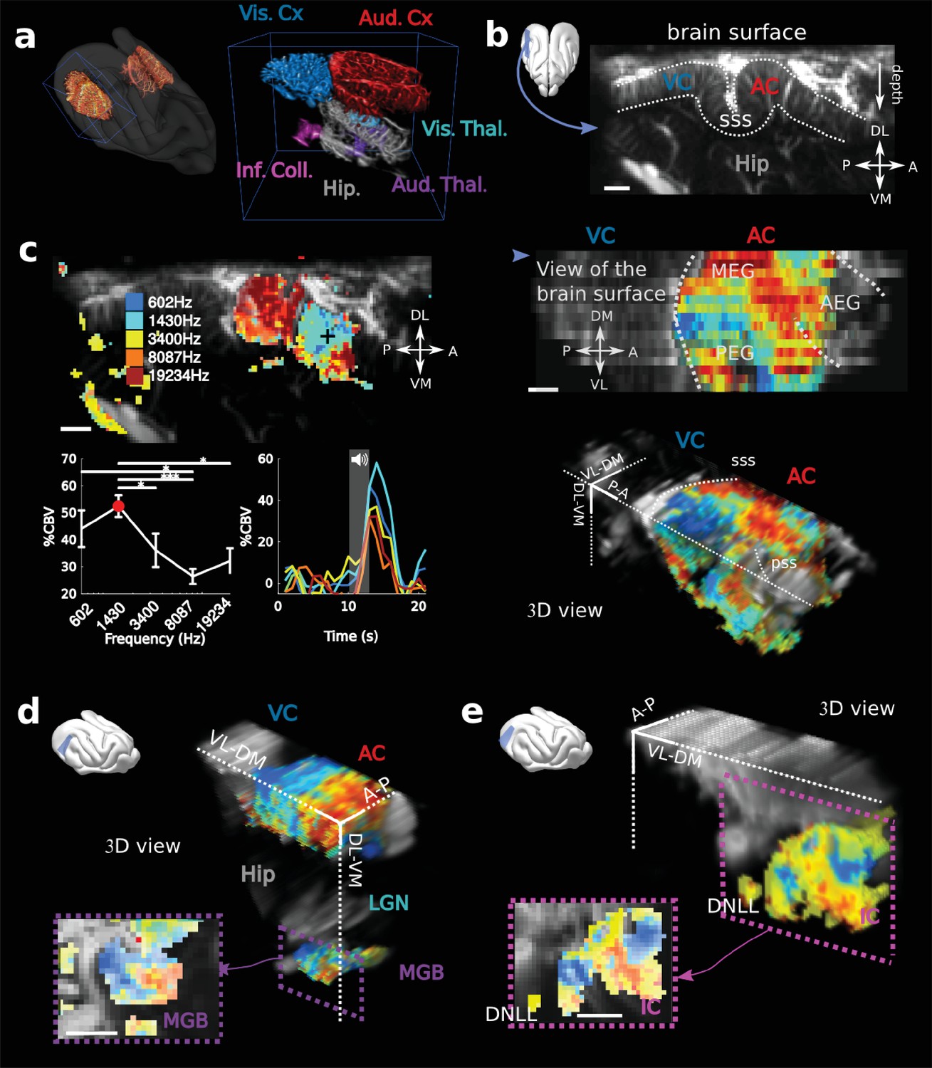
fUS imaging reveals the tonotopic organization of cortical, sub-cortical, and intracortical auditory structures in the awake ferret.
(a) Left: UFD-T of the left and right craniotomies, superimposed on an MRI scan of a ferret brain. Right: magnification of the blue bounding box (left). Auditory structures: auditory cortices (AC), medial geniculate body (MGB), inferior colliculus (IC). Other structures: hippocampus (Hip), visual cortex (VC). (b) Structural view of a tilted parasagittal slice (~30° from D-V axis) of the visual and auditory cortices (represented as a blue plane on the 3D brain). Lining delineates the cortex. (c) Upper left: Tonotopic organization of the slice described in (b). Lower left: tuning curve (mean ± sem) and average responses in %CBV (see Materials and methods) for the voxel located in the upper panel (black cross). Upper right: combination of 16 similar slices over the surface of the AC, arrow depicts slice of (b). AEG/MEG/PEG: anterior/middle/posterior ectosylvian gyrus. Lower right: 3D reconstruction of the whole AC’s functional organization. (d) 3D reconstruction of both the auditory cortex and auditory thalamus (non-tonotopic areas were masked on this reconstruction for clarity of the representation). Inset: single slice centered on the MGB. Its tonotopic axis runs along the PL-AM axis. Note that (b–d) were extracted from the left side of the brain, but flipped for visual clarity and coherence. (e) 3D reconstruction of the inferior colliculus and the dorsal nucleus of the lateral lemniscus (DNLL). Inset: single slice centered on the IC. Both (d) and (e) are tilted coronal slices (~30° from D-V axis). Their tonotopic axis runs along a ~ 20°-tilted D-V axis. All individual and converging scale bars: 1 mm. D: dorsal, V: ventral, M: medial, L: lateral, A: anterior, P: posterior.
Figure 1—figure supplement 1
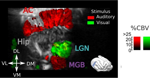
Responses to visual and auditory stimuli in the cortex and thalamus.
Tilted coronal slice (30° from D-V axis) over the AC and thalamus, showing hemodynamic responses evoked by a flickering light (green) or a broadband auditory noise (red) (map thresholded at +4 sem). Note that sound evoked activity in the most anterior part of the LGN can be visible (yellow color). Scale bar: 1 mm.
Figure 1—figure supplement 2
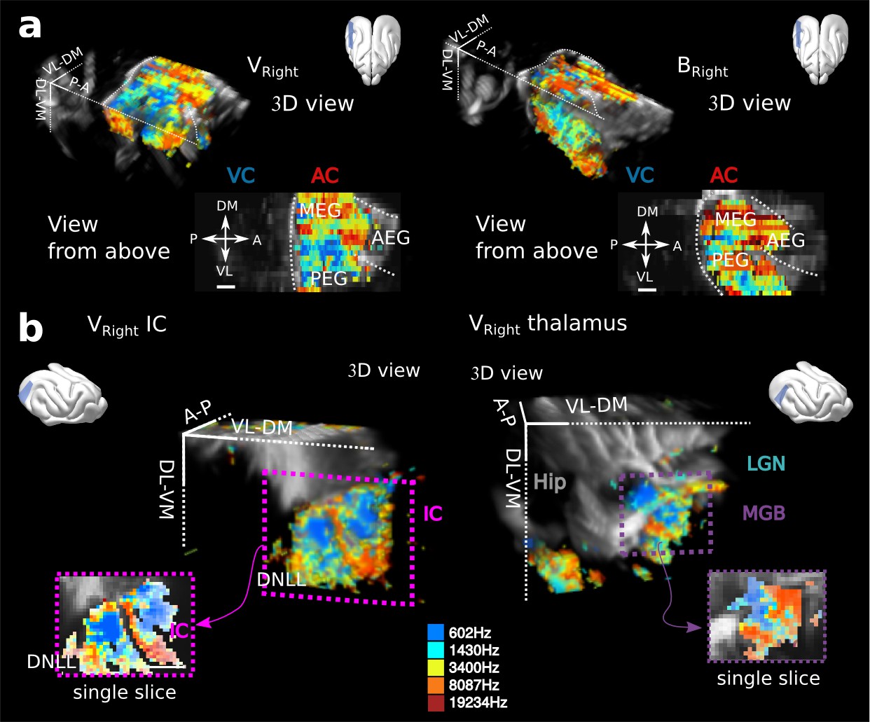
Tonotopies in AC, IC and MGB for other animals.
(a) 3D reconstructions and views from above for two other craniotomies, the right side of the one (named V) presented in Figure 1c, and another animal (B). Note the clear double reversal from MEG to PEG to VP in Bright. (b) Tonotopy for the IC in Vright (left), in which both IC and DNLL are visible, and the MGB in Vright (right). All tonotopic axis are consistent across craniotomies, even if substantial anatomical differences can be seen across animals, especially illustrated in the AC. Presented structures are oriented as tilted coronal sections (30° from D-V axis). All individual and converging scale bars: 1 mm.
Figure 1—figure supplement 3
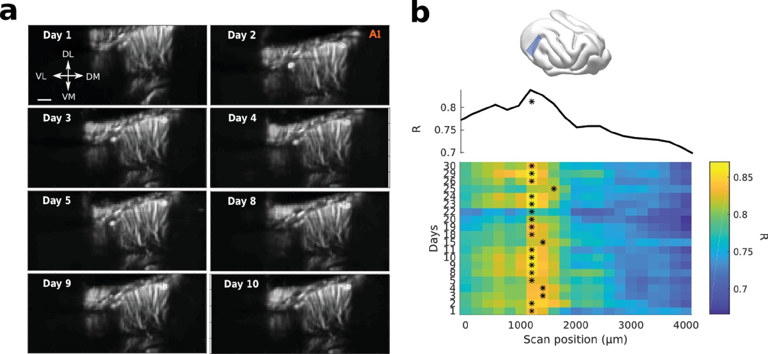
fUS allows for high recording stability and repositioning over days.
(a) Structural slices (tilted coronal slice, 30° from D-V axis, right hemisphere) over days, by repositioning the probe with a stereotaxic apparatus. Scale bar: 1 mm. (b) Recordings from the same slice were performed everyday for a long period of time. Each daily slice was repositioned in a vascular atlas previously obtained in the same animal, same craniotomy. The position is obtained by maximizing the correlation (R) between the new slice and the previous vascular atlas. Here the heatmap of R for different days (y-axis) correlated to different A-P regions of the atlas (x-axis) is shown. The star shows the maximum correlation for each day, and so the repositioning of the new slice (~1200 µm in that case). The upper panel shows R averaged over days.
Figure 2 with 3 supplements
Key features of fUS in awake animals: decoding accuracy, layer effect, and effective spatial resolution.
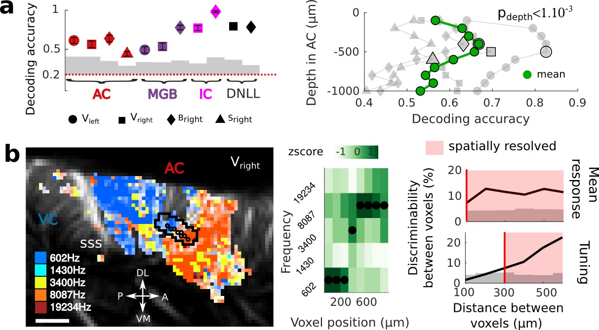
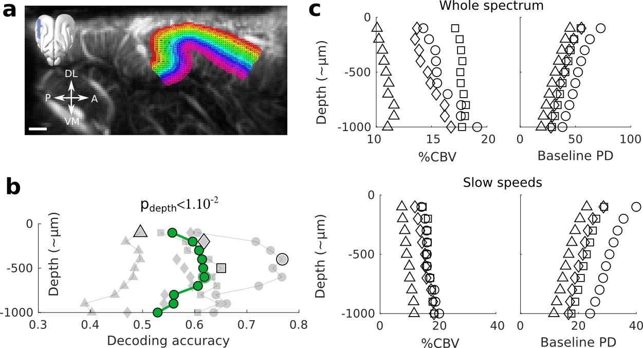
(a) Left panel: Decoding accuracy over the five frequencies, in different structures and different craniotomies (see legend). Grey histogram shows the upper limit for chance (p<1e-2, mean ±2 sem computed over 100 randomized decoding sessions). All structures showed significant decoding (p<1e-2). Right panel: decoding accuracy over depths, computed from the activity in the AC of 3 different animals (grey plots). All showed a similar profile, with the accuracy peaking between 400 and 500 µm. The green plot shows the average trend (repeated-measure ANOVA over depth, p<1e-3). (b) Left panel: example of a sharp tonotopic transition from low to high frequency, in the auditory cortex of Vright (map not smoothed). Scale bar: 1 mm. Middle panel: heatmap of the z-scored tuning curves of the consecutive voxels (shown by circles in left panel), with the best frequency indicated by a black dot, showing a shift from low to high frequency preference. Right panel: quantification of the lower spatial limit at which one can significantly find differences in the responsiveness (upper) or tuning (lower) of two voxels, with respect to their distance. Grey histogram shows the upper limit for chance (p<5e-2, 5% percentile over 50 randomizations). In that specific case, it was respectively 100 µm and 300 µm. The voxels used in this analysis are the ones within the black contour in left panel, centered on the sharp transition.
Figure 2—figure supplement 1
Controls for the decoding across depths.
(a) Example slice where the different depths are superimposed on the structural image. The upper part of the cortex was identifiable by the high density of vessels, while the lower part was approximated based on the end of vertical blood vessel, and distance to the surface (~1 mm). Note that with this definition, the first upper layer could accidentally contain some voxels within the pia. Scale bar: 1 mm. (b) Decoding across depths without focusing on the capillaries (whole spectrum). The same trend (p<1e-2) than in Figure 2a is visible, but less peaked and with lower accuracies. (c) Control measures of the %CBV (average maximum response over all frequencies) and baseline Power Doppler (PD, arbitrary unit) as a function of depth, indicating respectively the average responsiveness of each depth and its average baseline CBV. Upper panel: whole spectrum (no filtering). Lower panel: blood speeds above 3.1 mm.s−1 were filtered out, as in the main Figure 1f.
Figure 2—figure supplement 2

Single-slice recordings show high decoding possibility on an actual single-trial basis.
(a) Tonotopic organization of a tilted (30° from D-V axis) coronal slice of A1, over four consecutive days. A mask has been applied to focus on the tonotopic area. Scale bar: 1 mm. (b) PCA analysis over the averaged response for each frequency and all the voxels highlighted in (a), for the single slice designed by an arrowhead. Plotted here as plain lines are the mean hemodynamic response (starting from the center at sound onset, and increasing in all five directions), superimposed on the density of the peak responses at the single trial levels (N = 75 trials per frequency). Each frequency is designed by its color, and the intensity of the colored shading shows the density of trials displaying a response at this location. We can clearly see a separation of the different frequencies on a single-trial basis (reflected in the decoding analysis). (c) Decoding accuracy as a function of depth (slow speed vessels only). Left: different depth for the specific slice. Right: decoding accuracy peaks again around −400 µm, thus confirming that this effect could be observable on a single-slice basis. (d) Similar analysis as in (b), but this time the PCA is computed over the mean responses averaged over trials and daily sessions. The density map shows here the density of the peak responses at a single session level, averaged over all trials. The fact that densities are quite centered around the mean response suggests that all sessions have similar patterns of activity, and that tonotopic organization is relatively stable. (e) Decoding analysis as a function of depth, over days. Upper panel: mean decoding accuracy for all sessions (all blood vessel speeds). Heatmap shows the dependence of decoding accuracy on cortical depth. Stars show the peak of accuracy for each day, which is summed up in the right histogram showing the distribution of peak accuracy position. It clearly peaks around −300/400 µm, thus confirming our results over multiple recordings in the same slice. The blue arrowhead indicates the position of the slice shown in (c). Far right: mean decoding accuracy as a function of depth, averaged over days. The heterogeneity in decoding accuracy can be due to many parameters, such as small sample size and real biological variations.
Figure 2—figure supplement 3
Resolution quantification in other regions of the brain, and other animals.
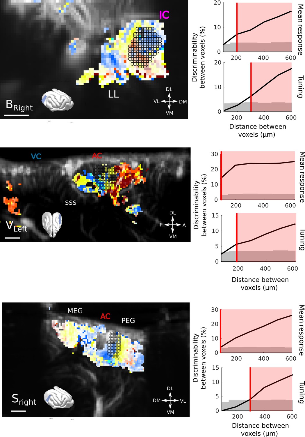
We performed the same analysis as shown in Figure 2b, in other regions and different animals. Overall, the obtained resolution are similar, that is, 100µm for responsiveness and 200–300 µm for tuning, within only 10 trials. (a) Quantification in the IC of Bright (10 trials). (b) Quantification in the AC of Vleft (10 trials). One can note here the heterogeneity of tunings within a small distance range. (c) Quantification in the AC of Sright (20 trials, coronal slice). All scale bars: 1 mm.
Figure 3 with 3 supplements

Exploring long-distance connectivity: the example of top-down projections from dlFC to the auditory system.
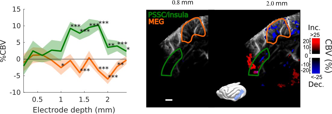
(a) Ferret brain with localization of electric stimulation (lightning) and site of fUS imaging shown in (b) (blue plane). A schematic of the electrical stimulation protocol (details in Materials and methods) is also shown in right panel. (b) FC-AC direct projection patterns revealed in fUS. Left: fUS imaging plane along the PSSC/insula, showing modulations of hemodynamic activity in MEG (orange delimitation) and PSSC/Insula (green delimitation) evoked by FC stimulation (map thresholded at +4 sem). The numbers 1 and 2 are here to help orientation. Right: %CBV in the 2 regions of interest after FC electric stimulation (highlighted in the left panel) with respect to the postero-anterior position of the stimulation electrode (0 represents 25.5 mm from caudal crest, 3 represents 28.5 mm), revealing a hot-spot of connectivity at about 1 mm (i.e 26.5 mm from caudal crest) (mean ±2 sem). ***: p-value<1e-3, **: p-value<1e-2, *: p-value<5e-2. Scale bar: 1 mm. (c) Ferret brain with localization of virus (tracer) injection site (green circle) with symbolized projections, and coronal slice represented in (d) (red plane). (d) Anatomical confirmation of connectivity. Left: bright field combined with fluorescence imaging, showing green fluorescent FC projections concentrated in the depth of the PSSC/insula and delineated anatomical structures (scale bar: 200 µm). Right: close-up of the labelled FC projection terminals in the PSSC/insula.
Figure 3—figure supplement 1
Frontal Cortex - Auditory cortex connectivity explored further: cortical depth.
Evoked responses in MEG/A1 and PSSC/Insula as a function of the vertical depth of the stimulation electrode (mean ±2 sem, map thresholded at +4 sem). Again, a hot spot of activation is found, suggesting that the bolus of activation triggered by our electrode does not exceed ~500 µm of a radius. Here, the 0 is set at the surface of the tissue covering the brain, that can be up to 1 mm thick. ***: p-value<1e-3, **: p-value<1e-2, *: p-value<5e-2. Scale bar: 1 mm.
Figure 3—figure supplement 2

Frontal Cortex - Auditory cortex connectivity explored further: secondary areas.
Scanning over the whole auditory MEG and PEG, showing that responses were evoked only in the fundus of the sulcus (map thresholded at +4 sem). Scale bar: 1 mm.
Figure 3—figure supplement 3
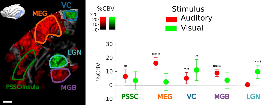
Frontal Cortex - Auditory cortex connectivity explored further: sound and vision.
Exploration of the multimodal responsiveness of the area. We played broadband noise (red) or flickering light (green) while recording the evoked %CBV in the same imaging plane. Scale bar: 1 mm. Left: overall responses for both visual and auditory stimulations (map thresholded at +2 sem). Anatomical regions of interest used for quantification are outlined. Right: mean evoked responses in these different regions. Note that the PSSC/insula was only weakly activated by sound, compared to MEG/A1. The part of the visual cortex shown here also presented bimodal responses, suggesting that this could be part of higher association areas such as area 21a of visual cortex or posterior parietal cortex. These experiments were performed on the same animal, but different days. Errorbars show mean ±2 sem. ***: p-value<1e-3, **: p-value<1e-2, *: p-value<5e-2.
Author response image 1

Author response image 2
Author response image 3
Author response image 4
Additional files
-
Transparent reporting form
- https://doi.org/10.7554/eLife.35028.014
Download links
A two-part list of links to download the article, or parts of the article, in various formats.
Downloads (link to download the article as PDF)
Open citations (links to open the citations from this article in various online reference manager services)
Cite this article (links to download the citations from this article in formats compatible with various reference manager tools)
Multi-scale mapping along the auditory hierarchy using high-resolution functional UltraSound in the awake ferret
eLife 7:e35028.
https://doi.org/10.7554/eLife.35028


