Temporal processing and context dependency in Caenorhabditis elegans response to mechanosensation
- Princeton University, United States
Figures
Figure 1 with 5 supplements
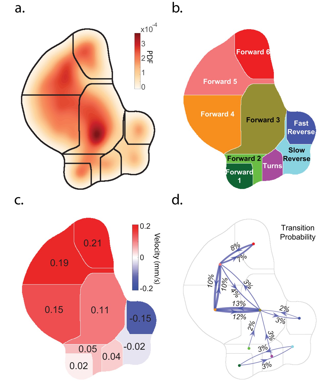
Caenorhabditis elegans behavior quantification.
(a) Behavior map showing the probability density of posture dynamics observed during 2284 animal-hours of behavior, including stimulus and control conditions (‘Random Noise’ row in Table 2). Posture dynamics have many dimensions but are projected down into a low-dimensional space using the t-SNE method used by Berman et al. (2014). Peaks indicate stereotyped postures. Discrete behavior states are defined by dividing the posture map into nine regions by using a watershedding algorithm. (b) Human-readable behavior names are provided by the experimenters. (c) Mean center of mass velocities of animals in each region. Positive velocity is in the direction of the animal’s head. (d) Probability of transitioning between behaviors. Thickness of lines scales with probability. Transition probabilities < 2% were omitted.
Figure 1—figure supplement 1
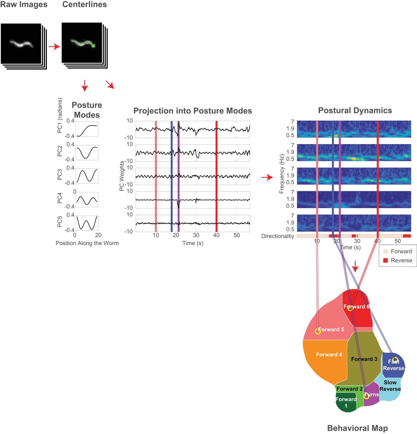
Analysis pipeline for classifying behavior.
Behavior is mapped and classified according to the animal’s posture dynamics, similar to the mapping described in Berman et al. (2014). Images of C. elegans are segmented to extract the animal’s centerline. Each centerline is projected into a linear combination of posture modes. The animal’s time-varying posture is represented as a time-series of corresponding weights. Spectrograms of these time-series describe the animal’s postural dynamics at each point in time. Posture dynamics are mapped into a two-dimensional plane using t-distributed stochastic neighbor embedding (t-SNE). The animal occupies a different point on the behavior map depending on its postural dynamics, and its placement in this map determines the behavioral classification.
Figure 1—figure supplement 2
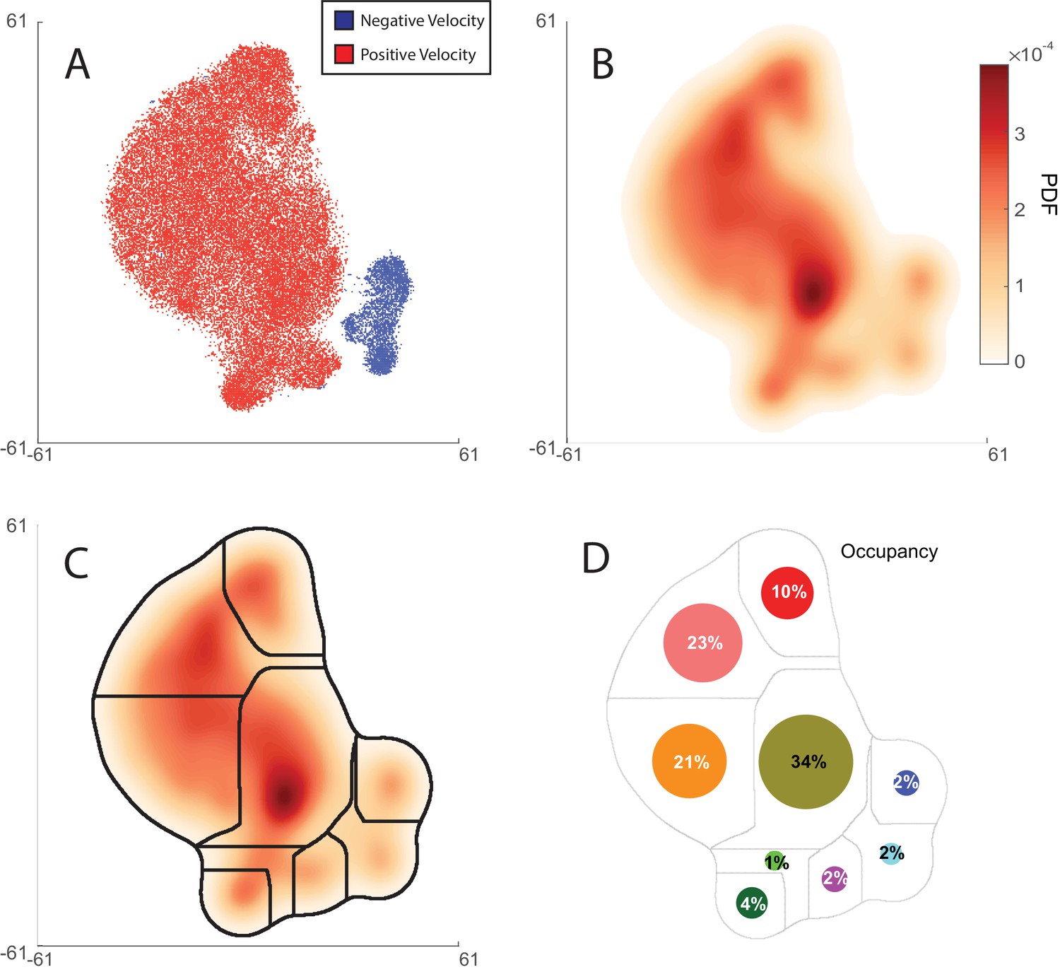
Behavior maps were generated from 2284 animal-hours of behavior recorded from Pmec-4::Chrimson worms during optogenetic stimulation and control conditions.
Distance between two points on the map is related to the Kullback-Leibler (KL) divergence of the respective posture dynamics spectra (Berman et al., 2014), but for our purposes here the axes can be taken as arbitrary. (a) The sign of the animal’s velocity is shown for 55,000 time-points uniformily selected from the recordings. Distinct regions in the map correspond to forward or backward locomotion. (b) Probability density plot showing the likelihood that the animal exhibits different behaviors. Peaks in the probability density correspond to stereotyped behaviors. (c) Natural boundaries that separate stereotyped worm behaviors are found using watershedding. Same as in Figure 1. These regions define distinct behavior states. (d) The probability of occupying a given behavior is shown for animals in an unstimulated condition. Circle area scales with occupancy probability.
Figure 1—video 1
Video of tracked animals undergoing optogenetic stimulation.
Movie showing worms undergoing random noise optogenetic stimulation. Image frames have been median filtered. Center of mass trajectories from the first step of the behavioral analysis are also shown. Trajectory colors are arbitrary. Inset shows the individual video of a single animal used for behavioral analysis. The red dot in the corner indicates the intensity of the optogenetic stimulus.
Figure 1—video 2
Videos of randomly selected animals performing each of the nine behaviors.
Randomly selected 3 s long examples of animals performing each of the nine behaviors.
Figure 1—video 3
Video showing the path of an animal through behavior space.
(Right)Video of an example animal. The detected centerline (green) is overlaid. A dot denotes the head. The animal is kept centered in the video, even though it is moving. (Left) Animal’s instantaneous behavior is shown (yellow ring) on the behavioral map.
Figure 2 with 4 supplements
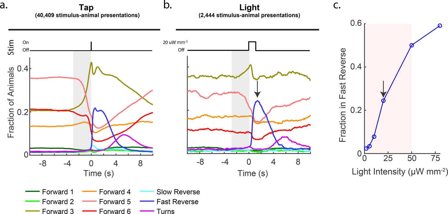
Stimulation evokes a diverse range of behavior responses.
(a) Fractions of animals occupying each behavior state in response to a plate tap (40,409 stimulus-animal presentations) and (b) in response to a 1 s optogenetic light stimulation of the six soft touch mechanosensory neurons (2,444 stimulus-animal presentations, 20 μW mm–2). Note the similarity in the behavior responses to light and tap. The gray shaded window indicates inherent temporal uncertainty in behavior classification. See 'Materials and methods'. (c) Response to optogenetic stimulation depends on light intensity. Peak fraction of animals in the 'Fast Reverse' state in a 6 s window post stimulus are shown for different-intensity light pulses. More than 2,000 stimulus-animal presentations were recorded for each point plotted. Arrow indicates the light intensity used in (B). Pink shaded region indicates light range used for subsequent continuous light stimulation experiments, as in Figure 3.
Figure 2—figure supplement 1
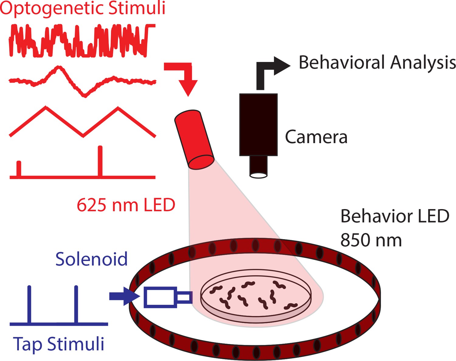
Diagram of high-throughput stimulation and behavior assay.
Worm behavior is recorded while delivering optogenetic or tap stimulation to a plate containing animals (mean standard deviation). Optogenetic stimulation is delivered by modulating the light intensity of three 625 nm LEDs (only one is shown in the diagram). Taps are delivered to the plate via a computer-controlled solenoid. Recordings last 30 min per plate, and each experimental series consists of many plates, see Table 2.
Figure 2—figure supplement 2
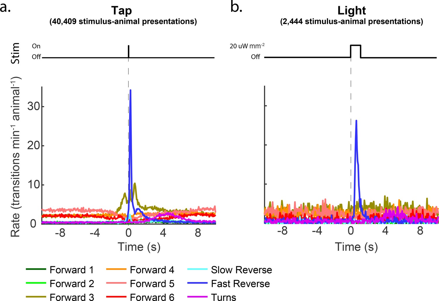
Transition rates for tap and light stimulation.
The rate of transitions into each behavior is shown aligned to a tap or 1 s optogenetic light stimulus. Panels (a) and (b) correspond to the occupancy plots in Figure 2a and b.
Figure 2—figure supplement 3
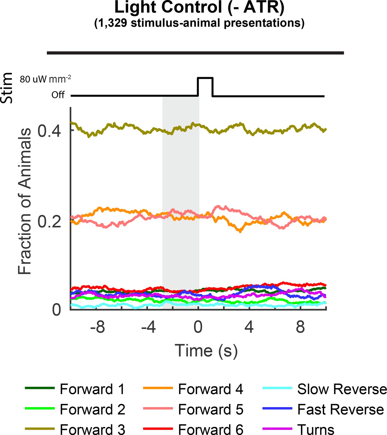
Control animals grown without ATR are light insensitive.
Fractions of control AML67 animals occupying each behavior state are shown in response to a light-pulse stimulus. Animals grown without the co-factor all-trans-retinal (– ATR) do not respond to light even at a light intensity level of 80 μW mm–2.
Figure 2—figure supplement 4
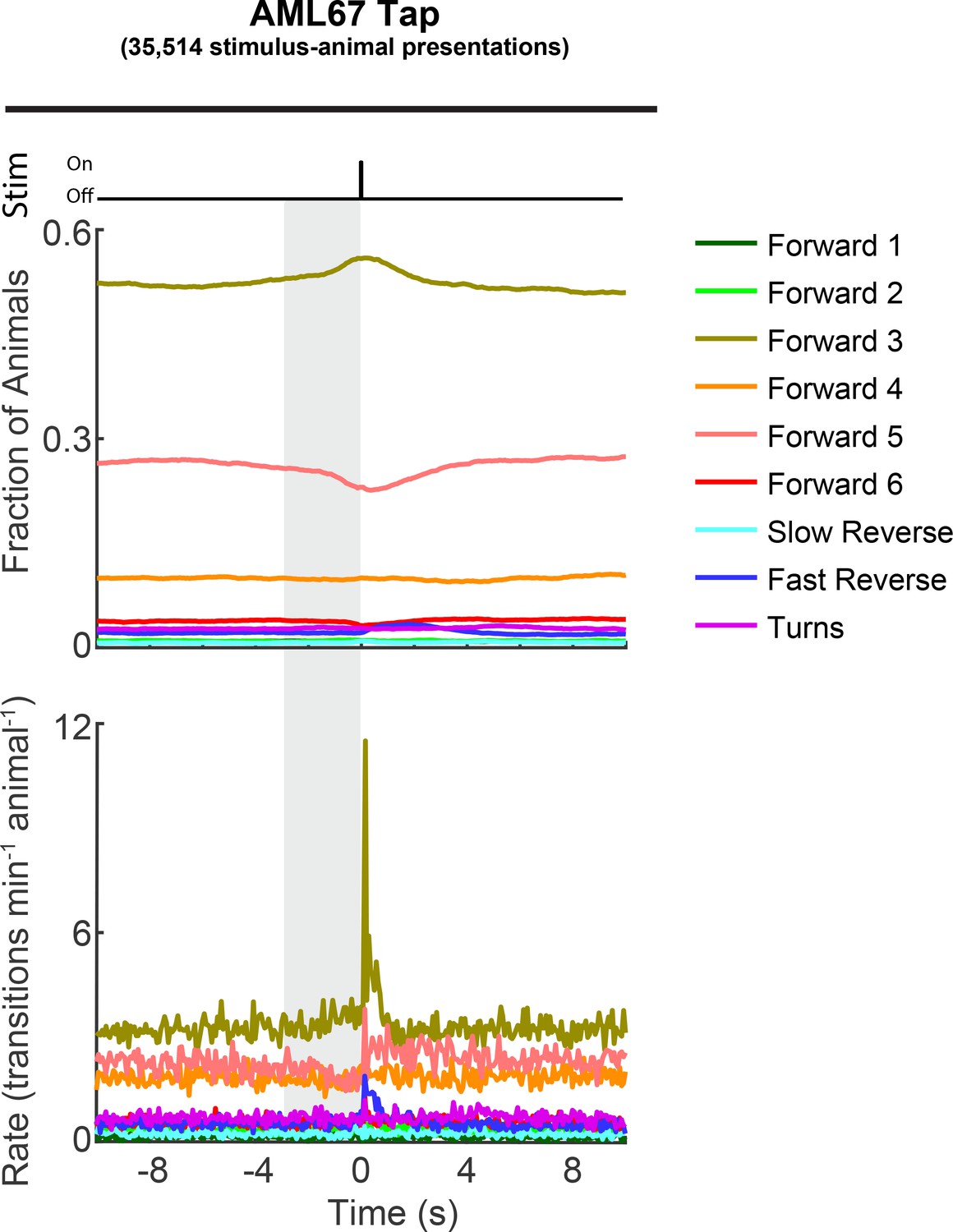
Tap sensitivity of transgenic animals is reduced compared to that of wild-type animals.
Fractions of AML67 animals occupying each behavior state and transition rates into each behavior are shown in response to a mechanical tap stimulus. Recordings from both ATR+ and ATR– conditions are pooled together. AML67 animals show decreased responsiveness to tap stimulation compared to wild-type, presumably because exogenous mec-4 promoter sequences deplete the transcription of endogenous MEC-4.
Figure 3 with 5 supplements
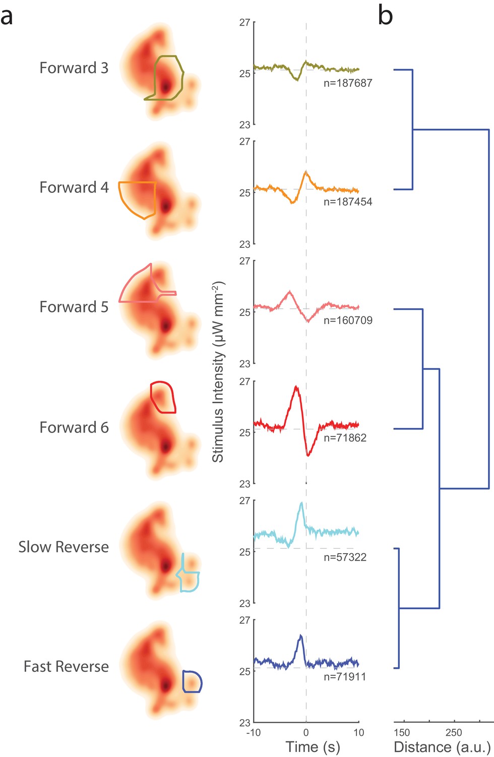
Transitions into behavior states are tuned to higher-order temporal features of the stimulus such as the derivative.
(a) Random noise time-varying light stimulus is delivered to a population of animals. Behavior-triggered averages (also referred to as kernels) are calculated for transitions into each behavior state from 1,784 animal-hours of recordings. Each behavior-triggered average describes features of the stimulus that correlate with that behavior transition. Only those behavior-triggered averages that pass a significance test in which they are compared to a shuffled stimuli are shown. The shape of the behavior-triggered average depends on the behavior. Note that some behaviors have Gaussian-like shapes, whereas others have biphasic shapes that act like derivatives. The numbers of observed transitions, , in each behavior are listed. (b) Similar behaviors have similar behavior-triggered averages. Dendrogram showing hierarchical clustering of the euclidian distance of the scaled behavior-triggered averages. The two reversal states, for example, form a cluster.
Figure 3—figure supplement 1
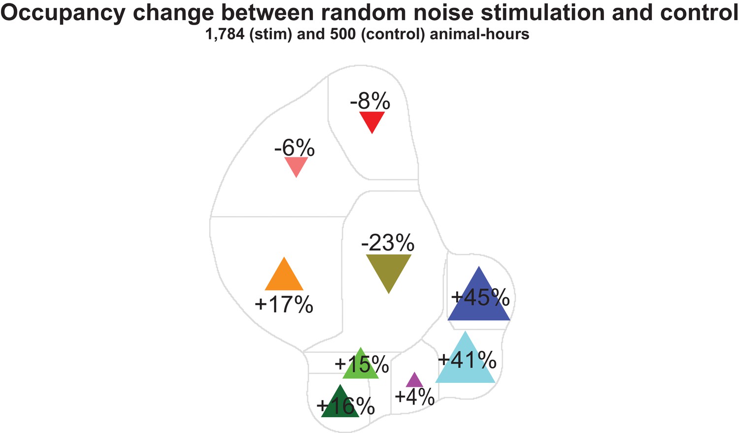
Change in behavioral occupancy evoked by random noise stimulation.
The change in occupancy during random noise optogenetic light stimulation (1,784 animal hours) compared to no-retinal (ATR–) control (500 animal-hours). Baseline occupancy during no-retinal control is shown in Figure 1—figure supplement 2d.
Figure 3—figure supplement 2
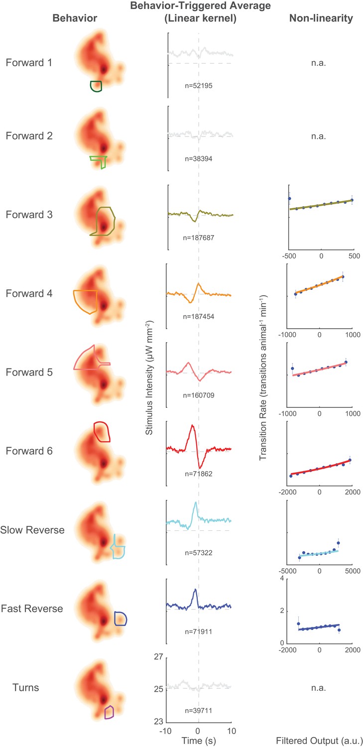
Behavior-triggered averages and non-linearities for all behaviors.
Behavior-triggered averages and associated non-linearities for transitions into all nine behavior states. Those behavior-triggered averages that fail to pass a shuffled significance threshold are shown in light gray. Non-linearities are only calculated for behaviors whose behavior-triggered averages pass our shuffled significance test. Note that the observed non-linearites (circles) are mostly well-approximated by a line (fitted line shown), consistent with the observation in Figure 2c that the animal responds roughly linearly in our stimulus regime.
Figure 3—figure supplement 3
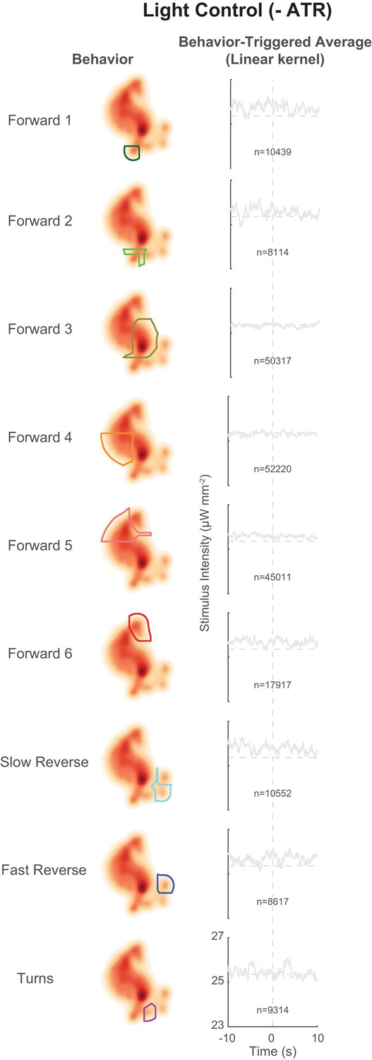
Behavior-triggered averages for control animals grown without ATR.
Behavior-triggered averages are shown for transitions into all nine behavior states for control animals grown without the required cofactor all-trans retinal (ATR–). As expected, none of the kernels pass a shuffled significance threshold. Consequently non-linearities were not calculated.
Figure 3—figure supplement 4
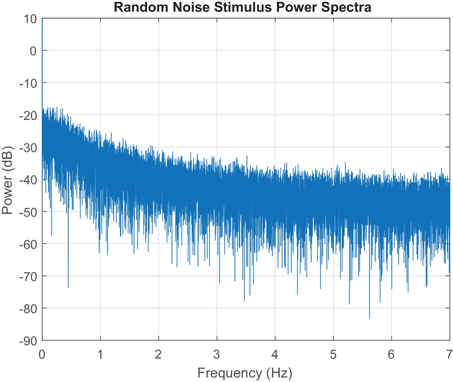
Power spectra of a single instantiation of the random noise stimulus.
The MATLAB periodogram function is used to generate the power spectra of the random noise stimulus for a 30 min experiment.
Figure 3—figure supplement 5
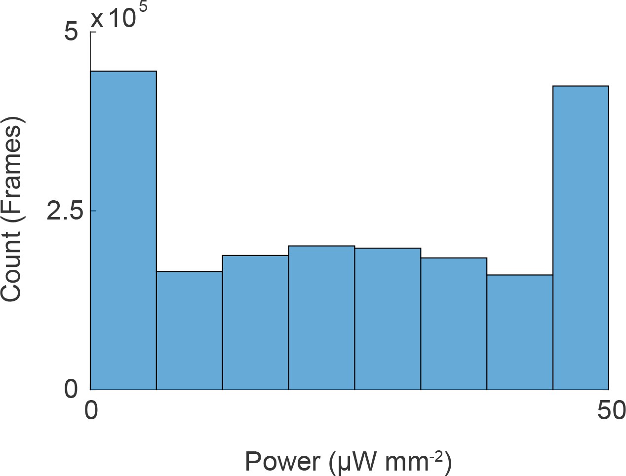
Light-intensity histogram for random noise stimulus.
A histogram of the light intensity at each time point for all random noise stimulus experiments.
Figure 4 with 2 supplements
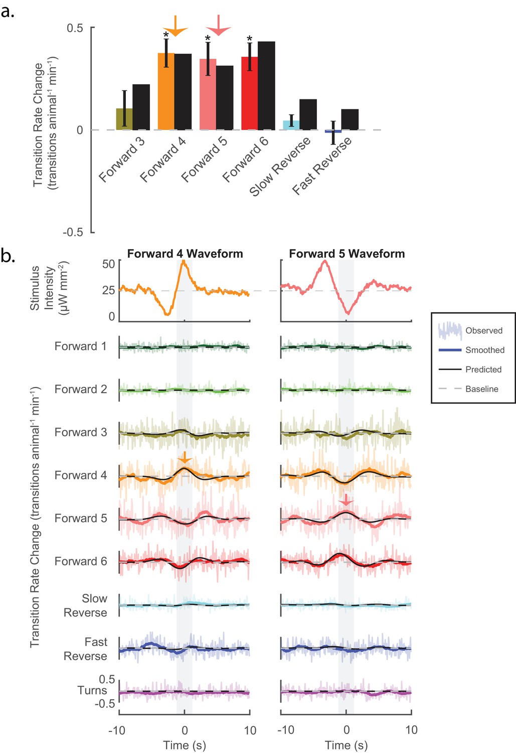
Stimuli can be tailored to elicit specific behavioral responses, and the LN model predicts such responses.
(a) Animals are presented with stimuli shaped like the kernels in Figure 3. Predicted (black bar) and observed (color bar) changes in transition rate are shown for transitions into each kernel-shaped stimulus’ corresponding behavior. For example, a 'Forward 3'-shaped stimulus increases transitions into 'Forward 3' (mustard bar). For five of the six behaviors, stimulation evoked increased transitions into their corresponding behaviors, as predicted. Transition rate changes are measured with respect to baseline (see 'Materials and methods'). Significance was estimated via a t-test and error bars show the standard error of the mean. The number of stimulus-animal presentations, from left to right, were 14,238, 13,612, 14,699, 14,424, 14,194 and 13,708. Of these, the number of timely transitions observed were 14,00, 1,428, 1,692, 944, 191 and 513. The p-values were 2.2e–1, 5.6e–6, 1e–4, 3.4e–5, 7.5e–2, 9.5e–1. (b) The LN model predicts details of the animal’s behavioral response. For each point in time, the LN model predicts the change from baseline of transition rates for all nine behaviors in response to a stimulus. Detailed responses to 'Forward 4'- and 'Forward 5'-kernel-shaped stimuli are shown (see Figure 4—figure supplement 1 for the rest). Raw transitions rates (light colored shading), smoothed transition rates (colored line) and LN prediction (solid black line) are shown. For stimuli that are shaped like 'Forward 4', the LN model correctly predicts not only that transitions into 'Forward 4' increase but also that transitions into 'Forward 5' and '6' decrease. Light gray shading indicates the 2 s time window used to calculate transition rates for the transitions shown in (A) (orange and pink arrows). Of 13,612 and 14,699 presentations for 'Forward 4'- and '5'-kernel shaped stimuli, respectively, the following number of transitions were observed in the 20 s window: by row for 'Forward 4'-shaped 1,265, 1,330, 12,312, 11,962, 13,436, 6,861, 1,735, 4,934 and 2,864, and for 'Forward 5'-shaped 1,198, 1,437, 13,657, 13,538, 14,656, 7,295, 1,673, 5,506 and 3,118.
Figure 4—figure supplement 1
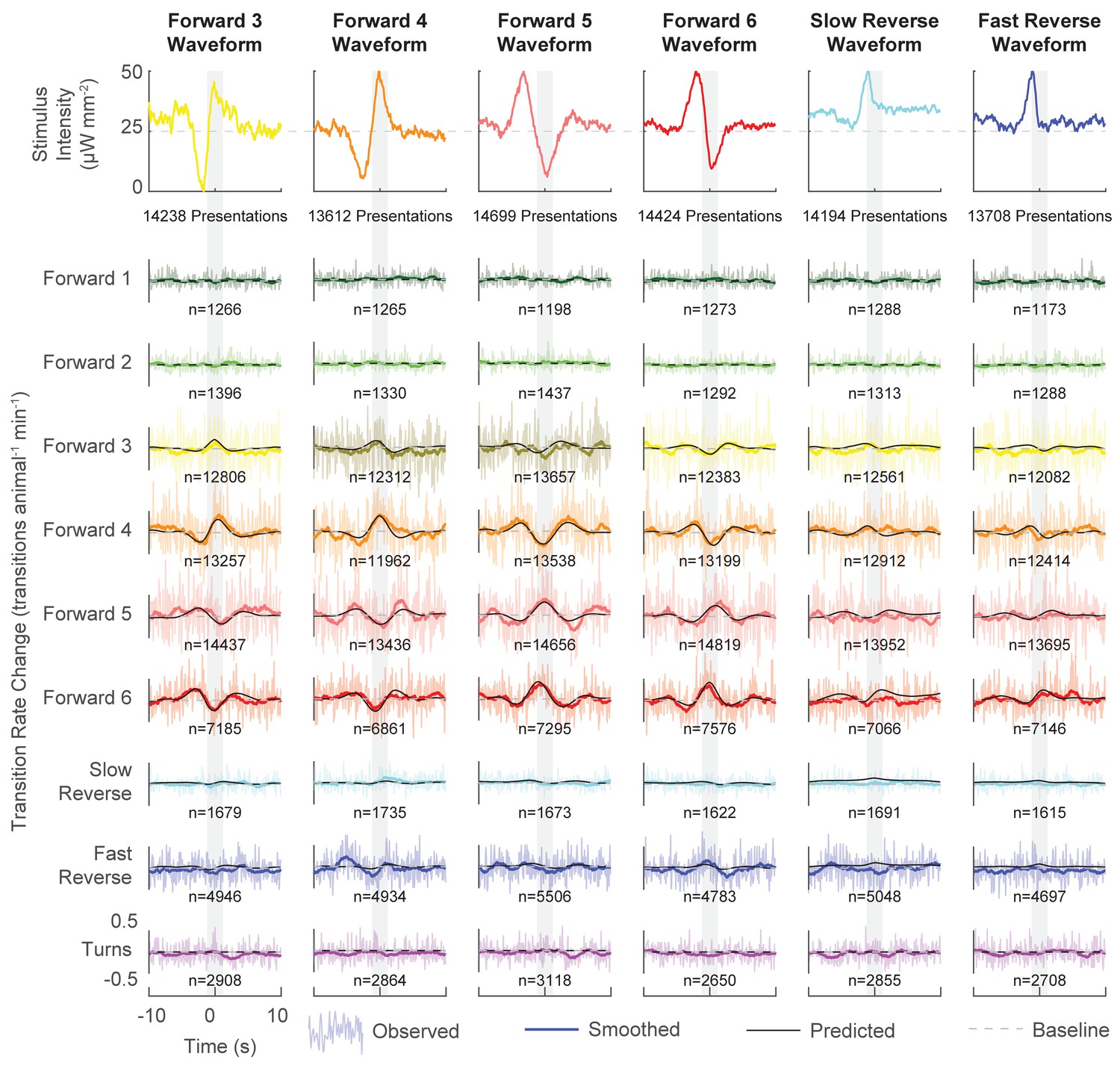
Behavioral responses to all kernel-shaped stimuli.
The LN model predicts the transition rate change from baseline for the nine behaviors in response to six stimuli constructed from statistically significant behavior-triggered averages. refers to the number of transitions of the corresponding behavior observed during the 20 s window. Presentation numbers refer to stimulus-animal presentations. The 'Forward 4' and 'Forward 5' columns are the same as those in Figure 4b.
Figure 4—figure supplement 2
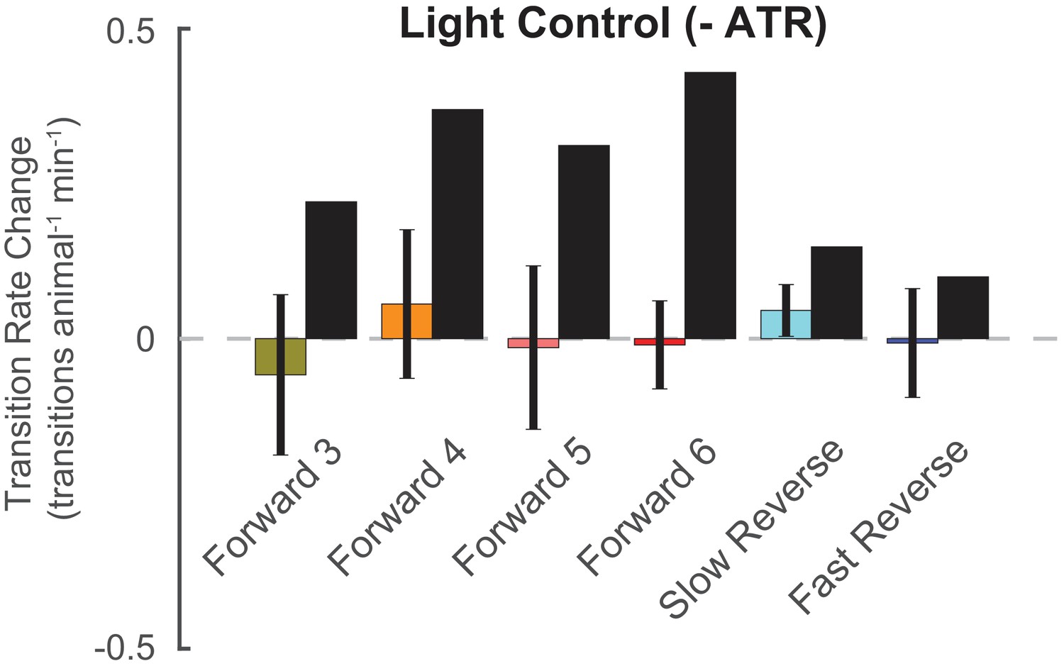
Control animals grown without ATR do not respond to kernel-shaped stimuli.
Kernel-shaped stimuli are delivered to AML67 control animals grown without the required co-factor ATR. The change in transition rate into the kernel-shaped stimuli’s corresponding behavior is shown, as in Figure 4a. Control animals do not exhibit a significant increase in transitions into the expected behavior states. Error bars show standard error of the mean. Black bars show LN predictions for light-sensitive animals. The number of stimulus-animal presentations, from left to right, were 3,474, 3,880, 3,988, 3,639, 4,351, and 3534. Of these, the number of timely transitions were 355, 225, 396, 162, 68, and 95. The p-values from a t-test were 0.63, 0.97, 0.92, 0.87, 0.33, and 0.68.
Figure 5 with 1 supplement
Novel stimuli can be constructed to enrich specific mechanosensory responses.
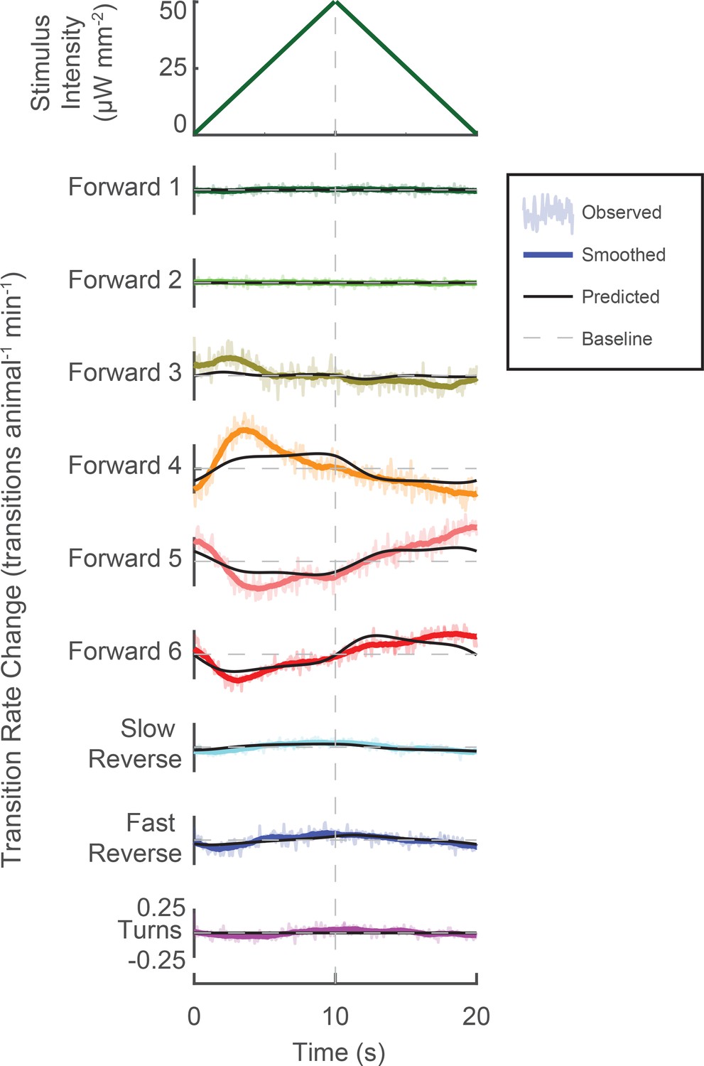
A novel triangle-wave optogenetic light stimulus was repeatedly presented to animals. Change in transition rates are shown for transitions into each behavior (raw, light color shaded; smoothed, solid color line). Changes to transition rate as predicted by the LN model are also shown (black line). Increasing light intensity increases transitions into 'Forward 3'and 'Forward 4', while decreasing light intensity increases transitions into 'Forward 5' and 'Forward 6'. Transitions into 'Slow Reverse' and 'Fast Reverse' are highest during greatest stimulus intensity. The LN model predicts these trends (though not all the details) even though the LN model was fitted using the random noise experiments and therefore was not exposed to this particular stimulus. In response to the 340,757 animal-stimulus presentations, the following number of transitions were observed (by row, from top to bottom): 33,315, 31,243, 298,400, 343,474, 327,509, 160,332, 43,909, 106,743, and 57,439.
Figure 5—figure supplement 1
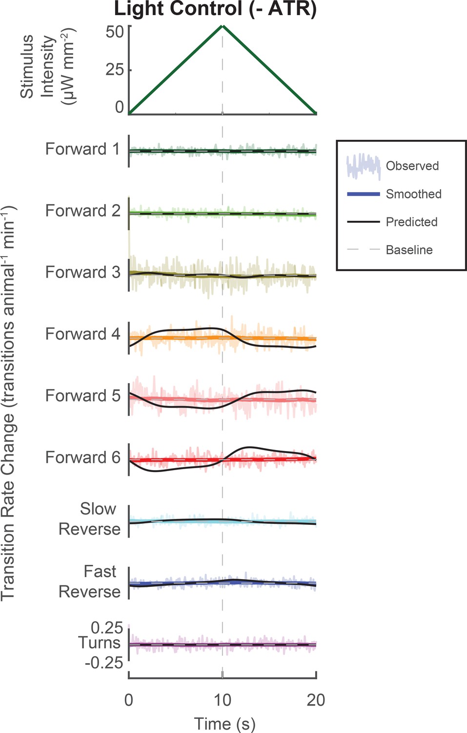
Control animals grown without ATR do not respond to triangle wave.
A novel triangle-wave optogenetic light stimulus, such as that in Figure 5, was repeatedly presented to control animals grown without the required co-factor retinal. Control animals do not respond to the stimulus. The observed response is shown as well as the LN predicted response. In reposnse to 142,461 animal-stimulus presentations, the following number of transitions were observed (by row, from top to bottom): 14,575, 15,886, 146,149, 82,216, 131,060, 42,080, 16,871, 18,581, and 28,318.
Figure 6 with 2 supplements
Behavior transitions that involve slowing down and speeding up have stereotyped tuning.
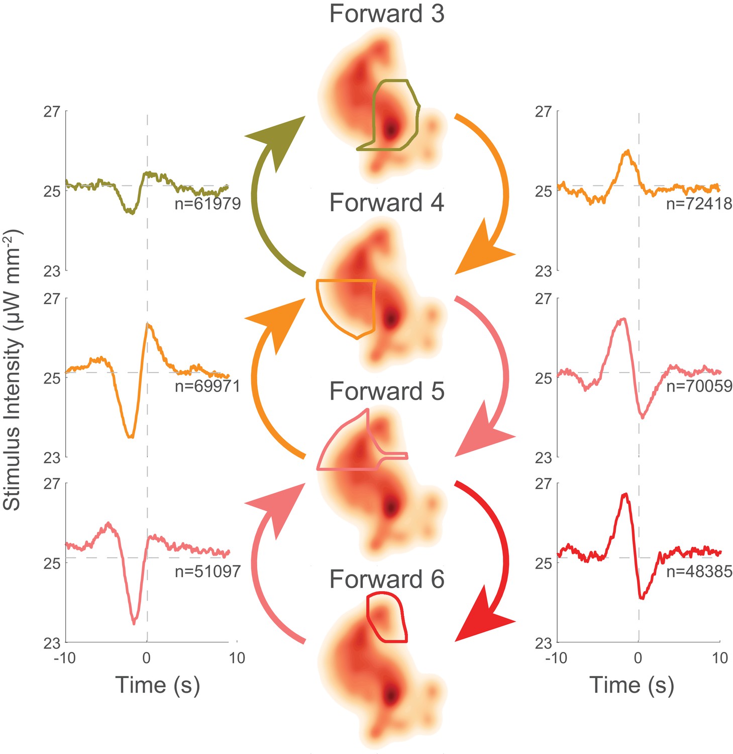
Selected context-dependent kernels are shown for transitions amongst forward locomotory states, where higher numbered states have higher velocities. Kernels for slowing transitions (left column) are all similar, whereas kernels for speeding up transitions (right column) are also similar. Slowing and speeding-up kernels resemble horizontal reflections of one another.
Figure 6—figure supplement 1
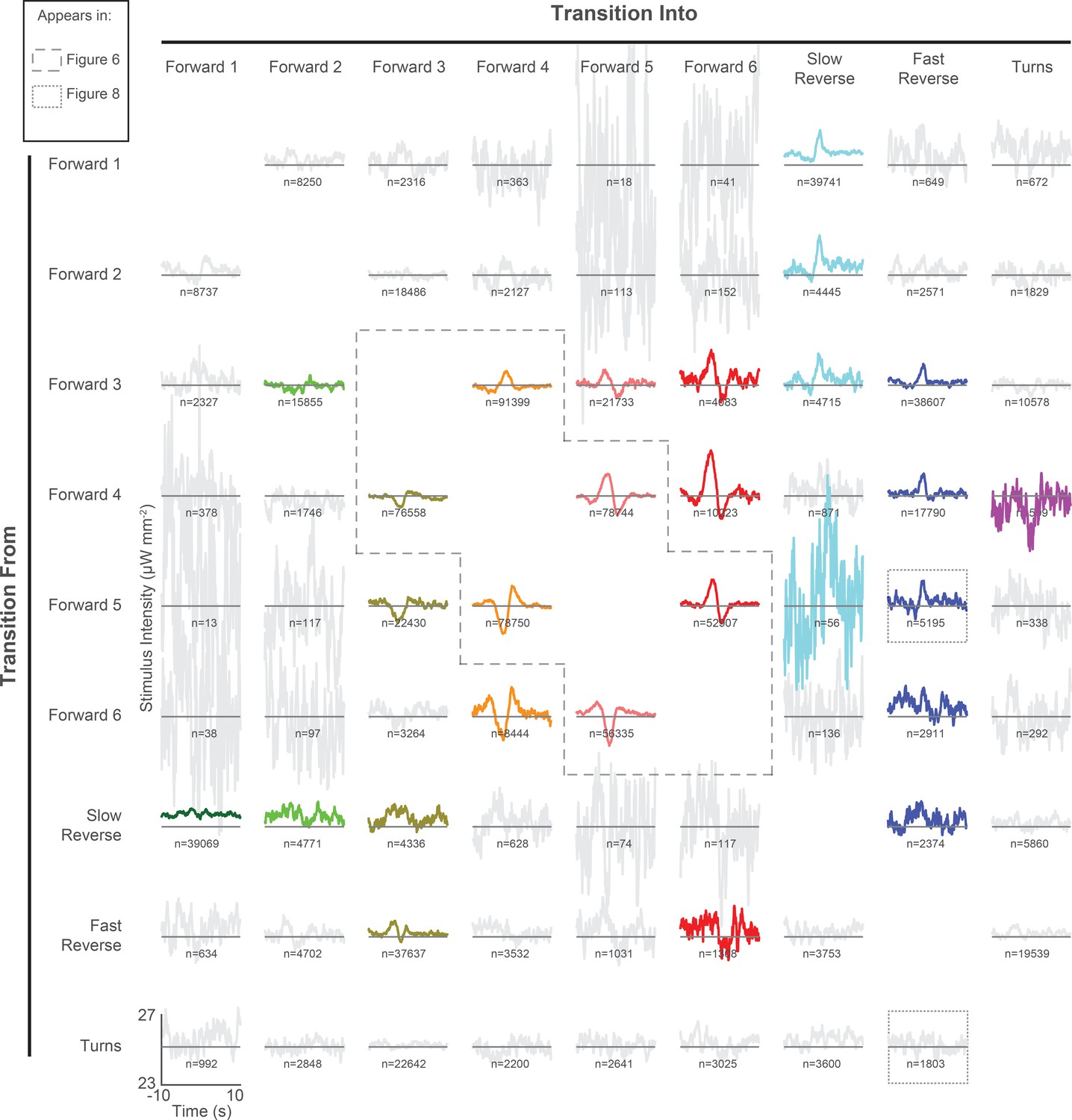
All 72 pairwise context-dependent behavior-triggered averages.
Pairwise behavior-triggered averages (also referred to as kernels) are shown for transitions from one specified behavior to another. Kernels are calculated from 1,784 animal-hours of continuous random noise stimulation (same as in Figure 3). For transitions into a given behavior (column), the kernel waveforms differ depending on the behavior that the animal originated in (rows). This suggests that the animal’s behavioral response to stimulus depends on the animal’s current behavior state. For each kernel, the vertical axis spans 23 to 27 μW mm–2 and the horizontal axis spans −10 to 10 s. indicates the number of transitions observed. Kernels that fail to pass a shuffled significance threshold are grayed out (see 'Materials and methods').
Figure 6—figure supplement 2
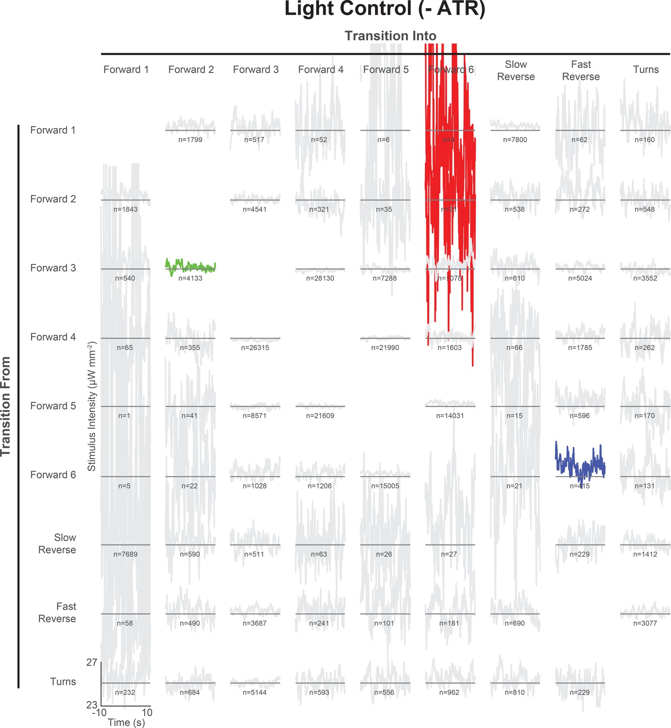
All 72 pairwise context-dependent behavior-triggered averages for control animals grown without ATR.
Pairwise behavior-triggered averages (also referred to as kernels) are shown for transitions from one specified behavior to another for control animals. For each kernel, the vertical axis spans 23 to 27 μW mm–2 and the horizontal axis spans −10 to 10 s. indicates the number of transitions observed. Kernels that fail to pass a shuffled significance threshold are grayed out (see 'Materials and methods').
Figure 7
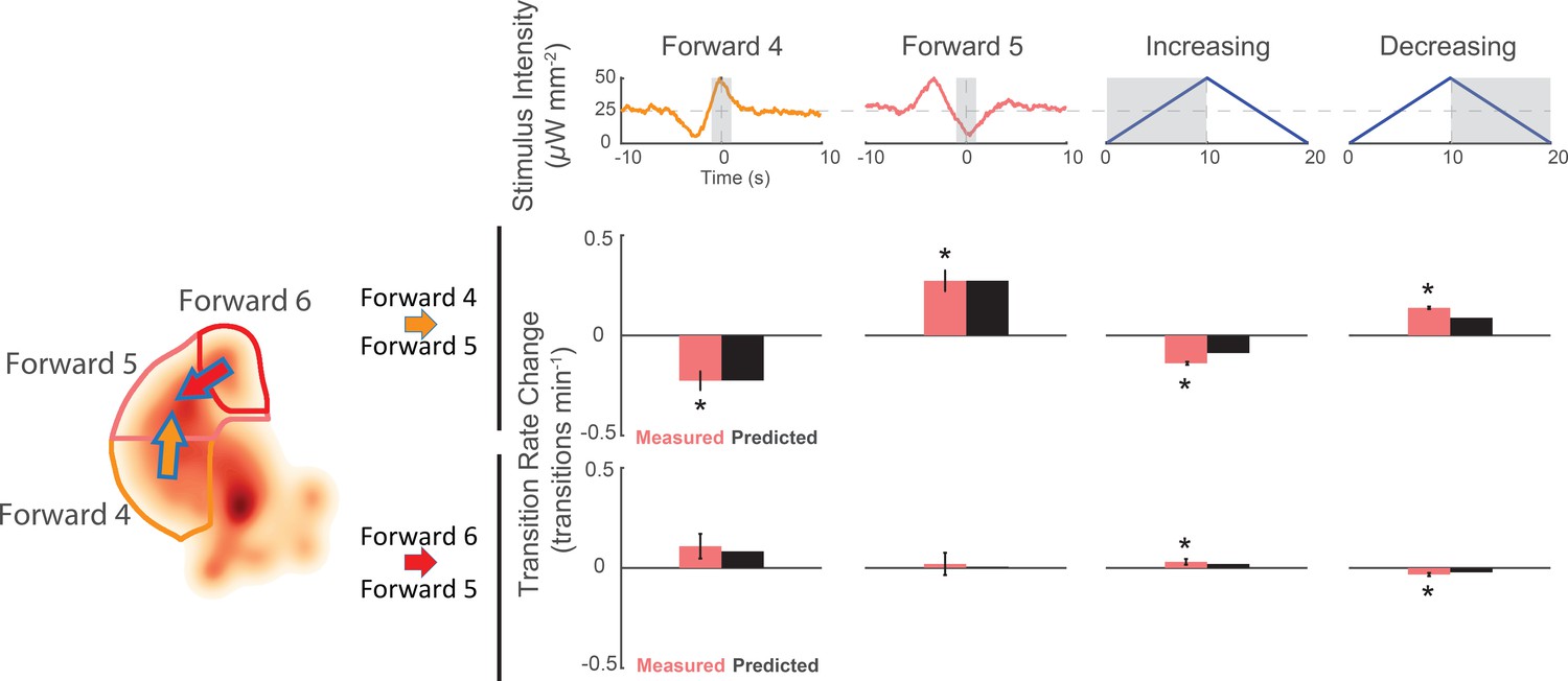
Animals respond to the same stimuli differently depending on their current behavior state.
The change in transition rate from baseline is shown for transitions into 'Forward 5' from either 'Forward 4 '(middle row) or 'Forward 6' (bottom row) in response to four different stimuli (columns). Observed transition rates (colored bars) are compared to LN model predictions (black bars). The stimulus affects the rate of transitions into 'Forward 5' differently depending on whether the animal was in 'Forward 4' or 'Forward 6' at the time of stimulus. For example, consistent with the animal responding to a slowing-down signal, the 'Forward 4'-shaped stimulus decreases 'Forward 4''Forward 5' transitions, but increases 'Forward 6''Forward 5' transitions. A star indicates a significant change in transition rate from baseline. Gray shaded regions indicate the time windows over which the transition rate is calculated. Baseline is defined slightly differently for the kernel-shaped stimuli compared to the triangle waves (see 'Materials and methods'). Of 13,612 and 14,699 stimulus-animal presentations for 'Forward 4' and 'Forward 5' kernel-shaped stimuli, and 340,757 stimulus-animal presentations for the triangle wave, the following number of transitions were observed: 26, 24, 2,604 and 2,634 for 'Forward 4''Forward 5' (top row) and 6, 7, 713 and 791 for 'Forward 6''Forward 5' (bottom row). A t-test was used to test for signifiant changes from baseline and the following p-values were observed: 5.5e–5, 6.9e–6, 1.8e–19 and 5.1e–48 for 'Forward 4'Forward 5' (top row) and 6.3e–2, 8.7e–1, 3.9e–2 and 6.7e–5 for 'Forward 6''Forward 5' (bottom row). Error bars show the standard error of the mean.
Figure 8 with 2 supplements
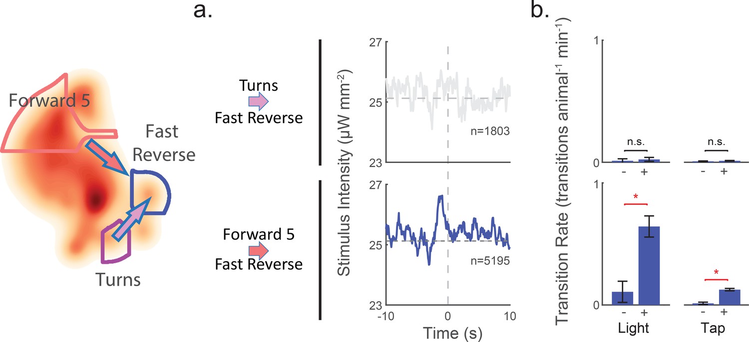
Attention to mechanosensory signals depends on behavior.
When the animal is in the 'Turn' state, it ignores mechanosensory stimuli. (a) Kernels are shown for two context-dependent transitions into 'Fast Reverse'. Transitions into 'Fast Reverse' originating from 'Forward 5' are correlated with stimulus and have a significant kernel, whereas those originating from 'Turn' are not correlated with stimulus and fail our shuffled significance threshold (see methods'). The kernels shown are same as those in Figure 6—figure supplement 1. (b) Transition rate in response to light and tap are shown. Animals in the 'Turn' state show no significant change in transition rates in response to light or tap, whereas animals in other states, such as 'Forward 5', do show a response. The 2 s post-stimulus mean transition rate into 'Fast Reverse' is shown in response to a 1 s light stimulation (+), mechanical tap (+) or a mock control (–). A star indicates significance, calculated using an E-test (see 'Materials and methods'). Error bars show the standard error of the mean. 2,487 and 37,000 stimulus-animal presentations were analyzed for light (+) and tap (+) respectively, and 2,427 and 40,012 mock controls(–) for light and tap. The following number of transitions were observed: 1, 2, 11 and 15 for 'Turns''Fast Reverse' (top row) and 9, 55, 18 and 160 for 'Forward 5''Fast Reverse' (bottom row). P-values for the E-test are 0.68 and 0.34 for 'Turn''Fast Reverse' (top row) and 1.96e-9 and 0 for 'Forward 5''Fast Reverse'(bottom row).
-
Figure 8—source data 1
P-values for transition rates in response to a light pulse for all pairwise transitions.
P-values are listed for the multiple hypothesis corrected E-tests performed in Figure 8—figure supplement 1. Row specifies ‘transition from’ and column specifies ‘transition into’.
- https://doi.org/10.7554/eLife.36419.032
-
Figure 8—source data 2
P-values for transition rates in response to a tap for all pairwise transitions.
P-values are listed for the multiple hypothesis corrected E-tests performed in Figure 8—figure supplement 2. Row specifies ‘transition from’ and column specifies ‘transition into’.
- https://doi.org/10.7554/eLife.36419.033
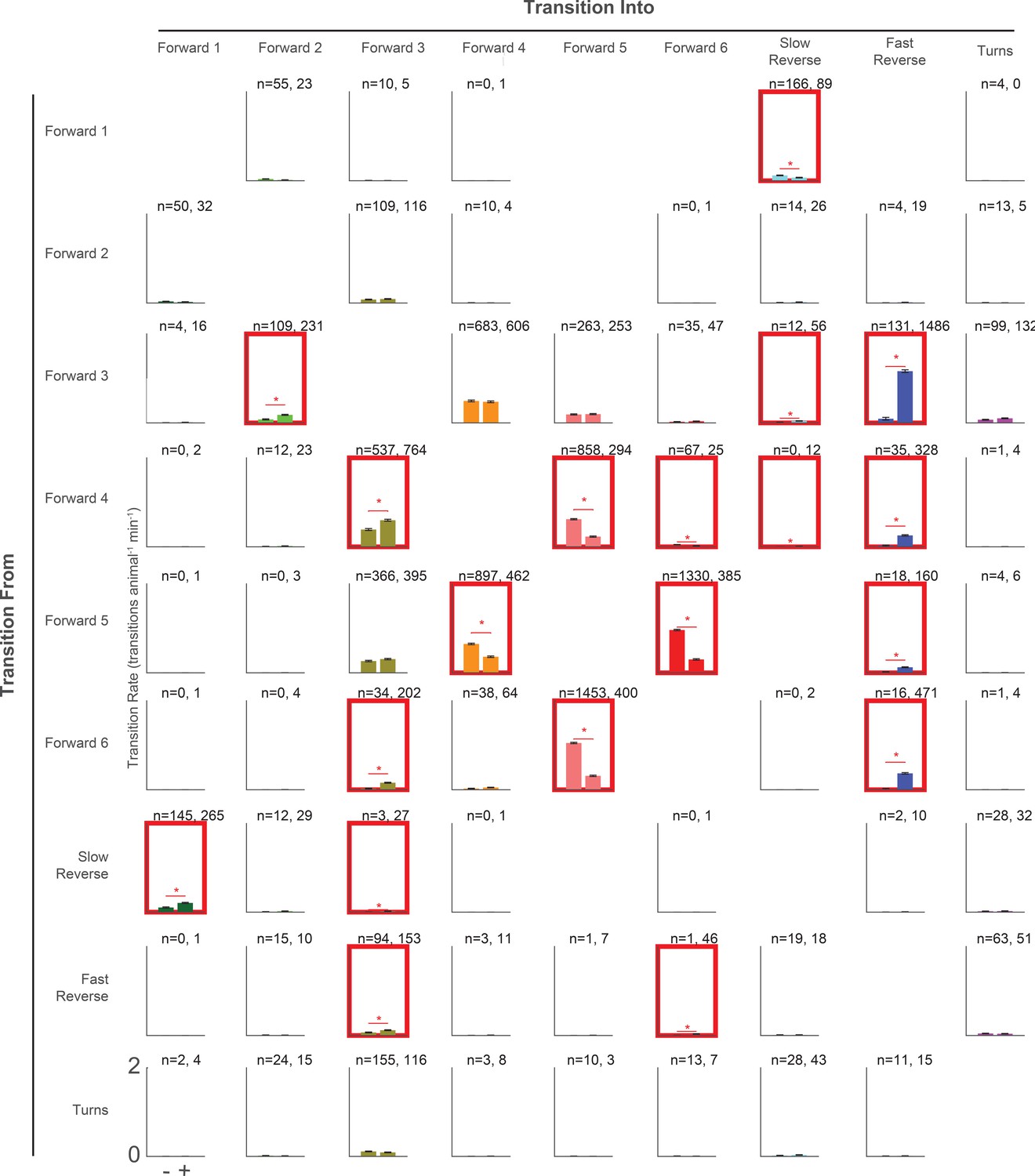
Figure 8—figure supplement 1

Transition rates in response to a light pulse for all pairwise transitions.
Transition rate is shown for all observed pairwise transitions in response to a 1 s light pulse (+, right bar, 2,487 stimulus-animal presentations) and mock control (–, left bar, 2,427 stimulus-animal presentations). The number of observed transitions for each bar is listed. No bars are shown for pairwise transitions that were not observed. The red boxes and stars indicate significance, calculated by a multiple hypothesis corrected E-test (see (Materials and methods'). P-values are listed in Figure 8—source data 1. Note that the axis range is 0 to 2 transitions animal–1 min–1 for all cases except for 'Forward 3''Fast Reverse', where it is 0 to 6 transitions animal–1 min–1.
Figure 8—figure supplement 2
Transition rates in response to a tap for all pairwise transitions.
Transition rate is shown for all observed pairwise transitions in response to tap (+, right bar, 37,000 stimulus-animal presentations) and mock control (–, left bar, 40,012 stimulus-animal presentations). The number of observed transitions for each bar is listed. No bars are shown for pairwise transitions that were not observed. Red boxes and stars indicate significance, calculated by a multiple hypothesis corrected E-test (see 'Materials and methods'). P-values are listed in Figure 8—source data 2. The axis range is always 0 to 2 transitions animal–1 min–1.
Tables
Table 1
Forward and reverse primer sequences used to generate pAL::pmec-4::Chrimson::SL2::mCherry::unc-54.
https://doi.org/10.7554/eLife.36419.034| Primer | Sequence |
|---|---|
| mec-4_fwd | AAGCTTCAATACAAGCTC |
| mec-4_rev | TAACTTGATAGCGATAAAAAAAATAG |
| CHRIMSON_fwd | ATGGCTGAGCTTATTTCATC |
| CHRIMSON_rev | AACAGTATCTTCATCTTCC |
| SL2_fwd | GGTACCGCTGTCTCATCC |
| SL2_rev | GATGCGTTGAAGCAGTTTC |
| mCherry_fwd | ATGGTCTCAAAGGGTGAAG |
| mCherry_rev | TTATACAATTCATCCATGCC |
| U54_fwd | GCGCCGGTCGCTACCATTAC |
| U54_rev | AAGGGCCCGTACGGCCGA |
Table 2
Summary of experimental conditions.
Each experimental series consisted of recordings of multiple plates usually spread across multiple days, as indicated. Recordings were all 30 mins in duration for each plate. Note that two methods were used to tally the number of stimulus-animal presentations (see 'Materials and methods'). Here, a stimulus presentation is counted even if the track was interrupted mid-presentation.
| Experiment series | Strain | Stim | ATR | Number of plates | Number of days | Interstimulus interval (s) | Stimulus duration (s) | Total animal- stimulus presentations | Cumulative Recording Length (animal-hours) | Animals per frame (Mean ± Stdev) | Figures |
|---|---|---|---|---|---|---|---|---|---|---|---|
| Random noise | AML67 | Light | + | 58 | 3 | n/a | n/a | n/a | 1,784 | 62 ± 34 | Figure 1, Figure 1—figure supplement 2, Figure 1—video 1, Figure 1—video 2, Figure 1—video 3, Figure 3, Figure 3—figure supplement 1, Figure 3—figure supplement 2, Figure 3—figure supplement 4, Figure 3—figure supplement 5, Figure 6, Figure 6—figure supplement 1, Figure 8 |
| − | 20 | 3 | n/a | n/a | n/a | 500 | 50 ± 23 | Figure 1, Figure 1—figure supplement 2, Figure 1—video 2, Figure 3—figure supplement 1, Figure 3—figure supplement 3, Figure 3—figure supplement 5, Figure 6—figure supplement 2 | |||
| Triangle wave | AML67 | Light | + | 62 | 3 | 0 | 20 | 340,757 | 1,912 | 62 ± 42 | Figure 5, Figure 7 |
| − | 20 | 3 | 0 | 20 | 142,461 | 800 | 80 ± 55 | Figure 5—figure supplement 1 | |||
| Kernel- shaped Stimuli | AML67 | Light | + | 44 | 3 | 40 | 20 | 84,875 | 1,453 | 66 ± 40 | Figure 4, Figure 4—figure supplement 1, Figure 7 |
| − | 12 | 3 | 40 | 20 | 22,866 | 392 | 65 ± 33 | Figure 4—figure supplement 1 | |||
| Light pulse | AML67 | Light | + | 12 | 1 | 59 | 1 | 15,128 | 260 | 43 ± 24 | Figure 2, Figure 8 |
| − | 6 | 1 | 59 | 1 | 8107 | 139 | 46 ± 18 | Figure 2—figure supplement 3 | |||
| Plate tap | AML67 | Tap | + | 7 | 2 | 60 | Impulse | 21,117 | 366 | 105 ± 60 | Figure 2—figure supplement 4 |
| − | 8 | 2 | 60 | Impulse | 14,646 | 254 | 64 ± 46 | ||||
| N2 | Tap | − | 22 | 3 | 60 | Impulse | 40,409 | 695 | 63 ± 25 | Figure 2, Figure 8, Figure 8—figure supplement 2 | |
| Total | 271 | 8,554 | 63 ± 40 |
Additional files
-
Transparent reporting form
- https://doi.org/10.7554/eLife.36419.036
Download links
A two-part list of links to download the article, or parts of the article, in various formats.
Downloads (link to download the article as PDF)
Open citations (links to open the citations from this article in various online reference manager services)
Cite this article (links to download the citations from this article in formats compatible with various reference manager tools)
Temporal processing and context dependency in Caenorhabditis elegans response to mechanosensation
eLife 7:e36419.
https://doi.org/10.7554/eLife.36419


