Figures and data in Learning recurrent dynamics in spiking networks | eLife

Figures
Additional files

7 figures and 1 additional file

Figures

Figure 1 with 2 supplements

Download asset Open asset

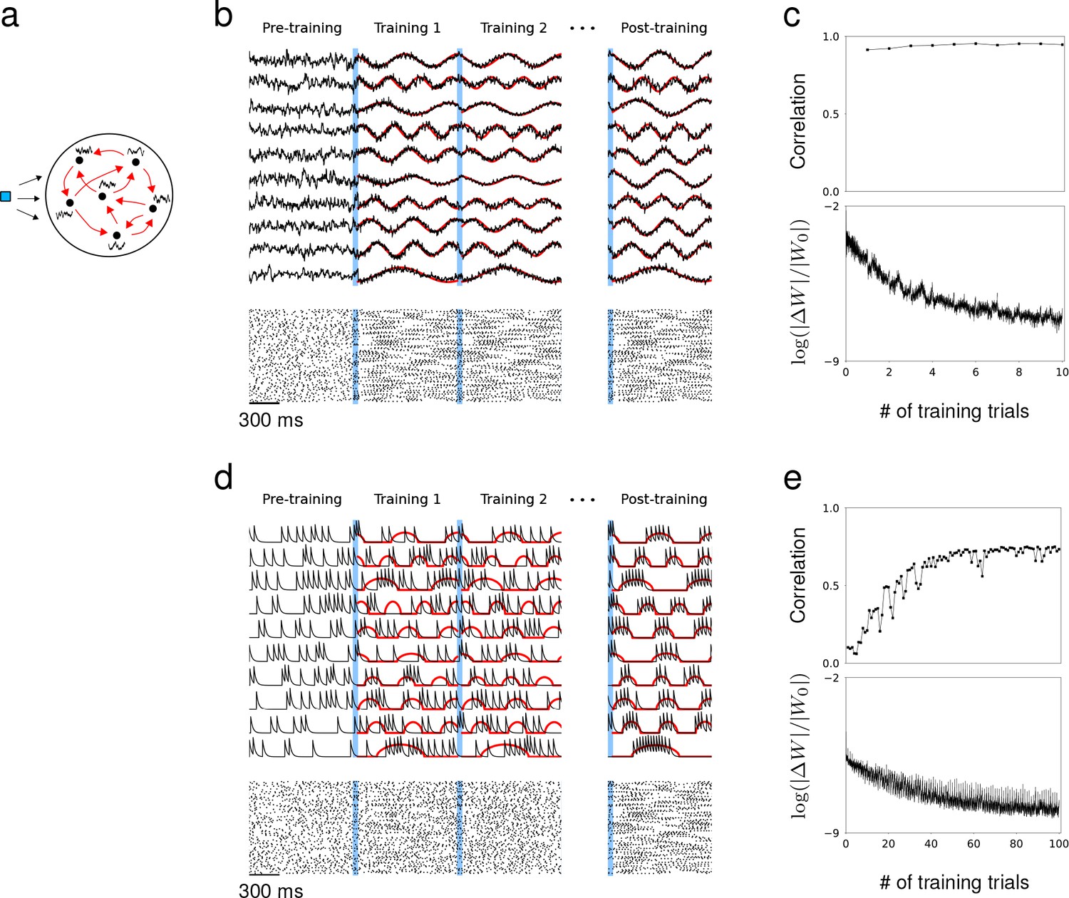
Synaptic drive and spiking rate of neurons in a recurrent network can learn complex patterns.

(a) Schematic of network training. Blue square represents the external stimulus that elicits the desired response. Black curves represent target output for each neuron. Red arrows represent recurrent connectivity that is trained to produce desired target patterns. (b) Synaptic drive of 10 sample neurons before, during and after training. Pre-training is followed by multiple training trials. An external stimulus (blue) is applied prior to training for 100 ms. Synaptic drive (black) is trained to follow the target (red). If the training is successful, the same external stimulus can elicit the desired response. Bottom shows the spike rater of 100 neurons. (c) Top, The Pearson correlation between the actual synaptic drive and the target output during training trials. Bottom, The matrix (Fresenius) norm of changes in recurrent connectivity normalized to initial connectivity during training. (d) Filtered spike train of 10 neurons before, during and after training. As in (b), external stimulus (blue) is applied immediately before training trials. Filtered spike train (black) learns to follow the target spiking rate (red) with large errors during the early trials. Applying the stimulus to a successfully trained network elicits the desired spiking rate patterns in every neuron. (e) Top, Same as in (c) but measures the correlation between filtered spike trains and target outputs. Bottom, Same as in (c).

https://doi.org/10.7554/eLife.37124.002

Figure 1—figure supplement 1

Download asset Open asset

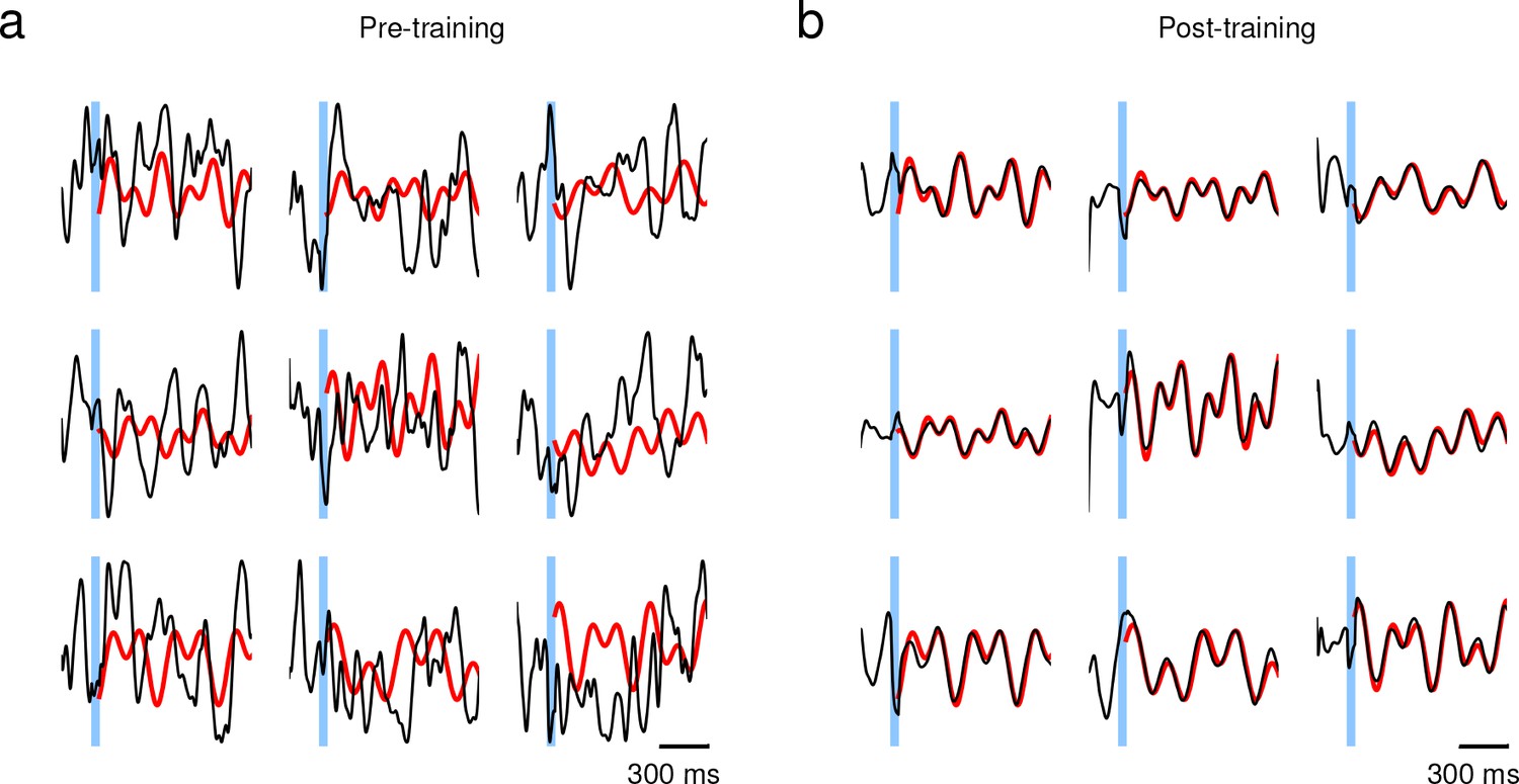
Learning arbitrarily complex target patterns in a network of rate-based neurons.

The network dynamics obey $τ {\dot{x}}_{i} = - x_{i} + \sum_{j = 1}^{N} W_{i j} r_{j} + I_{i}$ where $r_{j} = t a n h (x_{j})$ . The synaptic current $x_{i}$ to every neuron in the network was trained to follow complex periodic functions $f (t) = A s i n (2 π (t - T_{0}) / T_{1}) s i n (2 π (t - T_{0}) / T_{2})$ where the initial phase $T_{0}$ and frequencies $T_{1}, T_{2}$ were selected randomly. The elements of initial connectivity matrix $W_{i j}$ were drawn from a Gaussian distribution with mean zero and standard deviation $σ / \sqrt{N p}$ where $σ = 2$ was strong enough to induce chaotic dynamics; Network size $N = 500$ , connection probability between neurons $p = 0.3$ , and time constant $τ = 10$ ms. External input $I_{i}$ with constant random amplitude was applied to each neuron for 50 ms (blue) and was set to zero elsewhere. (a) Before training, the network is in chaotic regime and the synaptic current (black) of individual neurons fluctuates irregularly. (b) After learning to follow the target trajectories (red), the synaptic current tracks the target pattern closely in response to the external stimulus.

https://doi.org/10.7554/eLife.37124.003

Figure 1—figure supplement 2

Download asset Open asset

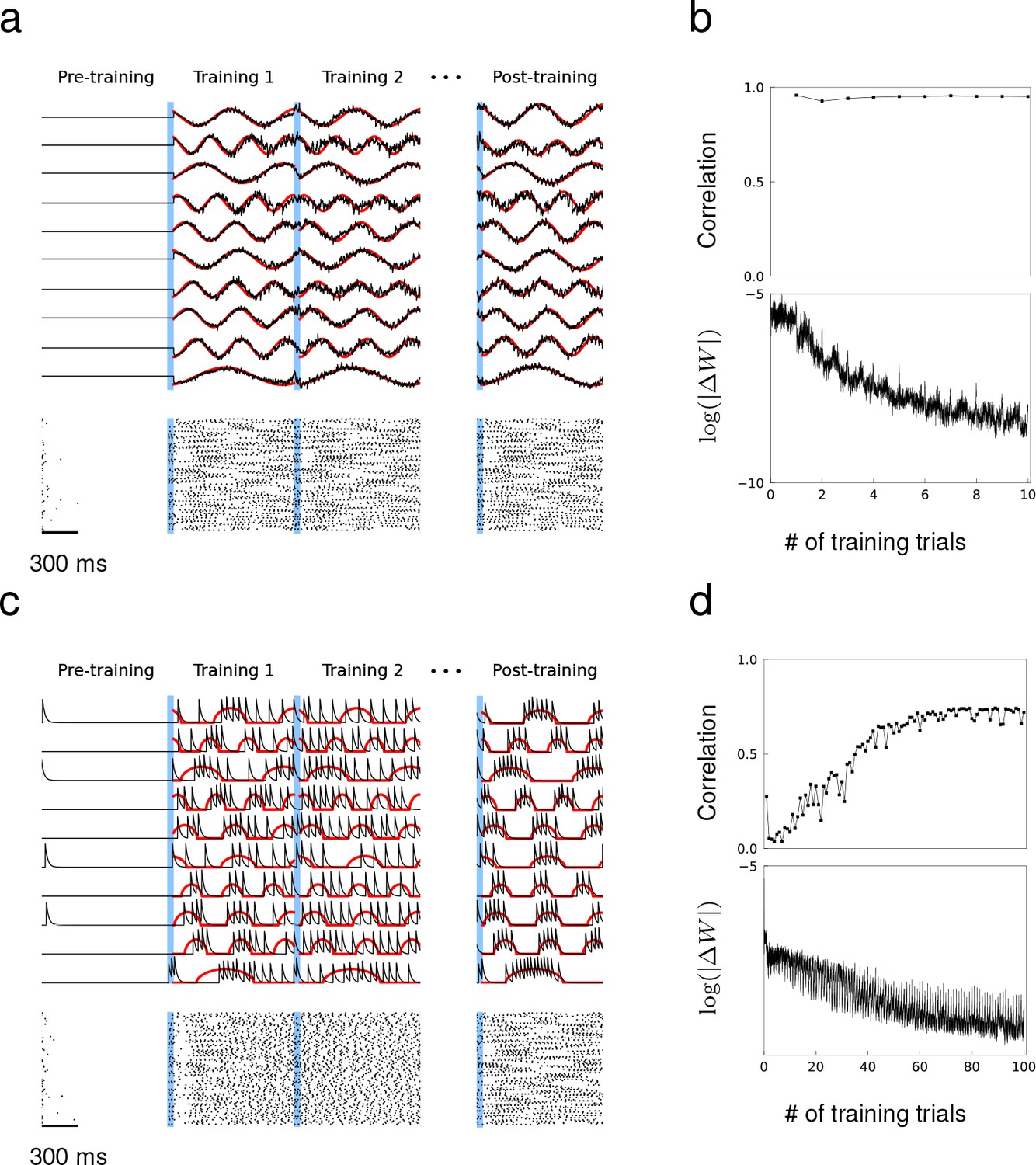
Training a network that has no initial connections.

The coupling strength of the initial recurrent connectivity is zero, and, prior to training, no synaptic or spiking activity appears beyond the first few hundred milliseconds. (a) Training synaptic drive patterns using the RLS algorithm. Black curves show the actual synaptic drive of 10 neurons and red curves show the target outputs. Blue shows the 100 ms external stimulus. (b) Correlation between synaptic drive and target function (top) and the Frobenius norm of changes in recurrent connectivity normalized to initial connectivity during training (botom). (c and d) Same as in (a) and (b), but spiking rate patterns are trained.

https://doi.org/10.7554/eLife.37124.004

Figure 2

Download asset Open asset

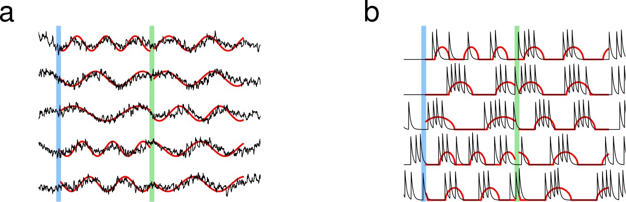
Learning multiple target patterns.

(a) The synaptic drive of neurons learns two different target outputs. Blue stimulus evokes the first set of target outputs (red) and the green stimulus evokes the second set of target outputs (red). (b) The spiking rate of individual neurons learns two different target outputs.

https://doi.org/10.7554/eLife.37124.005

Figure 3 with 3 supplements

Download asset Open asset

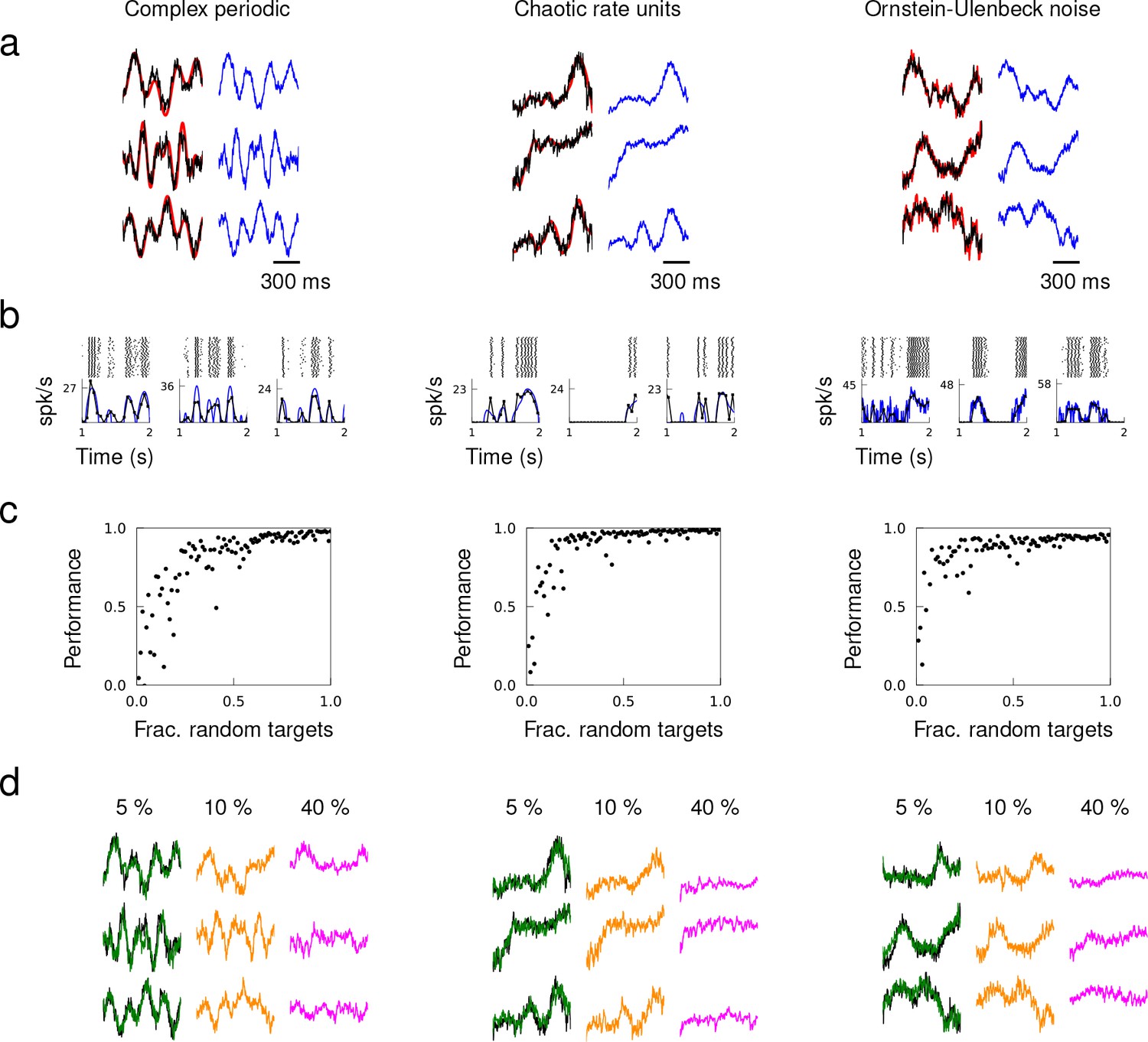
Quasi-static and heterogeneous patterns can be learned.

Example target patterns include complex periodic functions (product of sines with random frequencies), chaotic rate units (obtained from a random network of rate units), and OU noise (obtained by low-pass filtering white noise with time constant 100 ms). (a) Target patterns (red) overlaid with actual synaptic drive (black) of a trained network. Quasi-static prediction (Equation 1) of synaptic drive (blue). (b) Spike trains of trained neurons elicited multiple trials, trial-averaged spiking rate calculated by the average number of spikes in 50 ms time bins (black), and predicted spiking rate (blue). (c) Performance of trained network as a function of the fraction of randomly selected targets. (d) Network response from a trained network after removing all the synaptic connections from 5%, 10% and 40% of randomly selected neurons in the network.

https://doi.org/10.7554/eLife.37124.006

Figure 3—figure supplement 1

Download asset Open asset

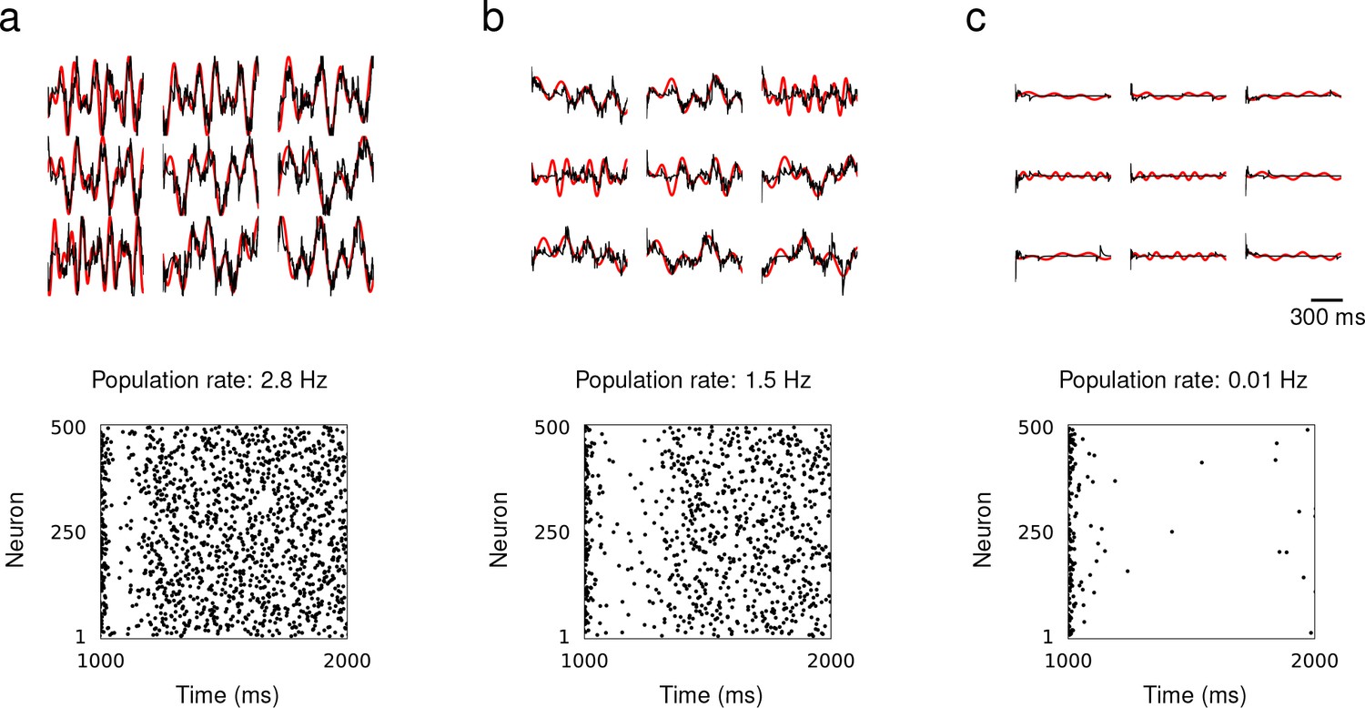
Learning target patterns with low-population spiking rate.

The synaptic drive of networks consisting of 500 neurons were trained to learn complex periodic functions $f (t) = A s i n (2 π (t - T_{0}) / T_{1}) s i n (2 π (t - T_{0}) / T_{2})$ where the initial phase $T_{0}$ and frequencies $T_{1}, T_{2}$ were selected randomly from [500 ms, 1000 ms]. (a) The amplitude $A = 0.1$ , resulting in population spiking rate 2.8 Hz in trained window. (b) The amplitude $A = 0.05$ , resulting in population spiking rate 1.5 Hz in trained window. (c) The amplitude $A = 0.01$ , resulting in population spiking rate 0.01 Hz in trained window and learning fails.

https://doi.org/10.7554/eLife.37124.007

Figure 3—figure supplement 2

Download asset Open asset

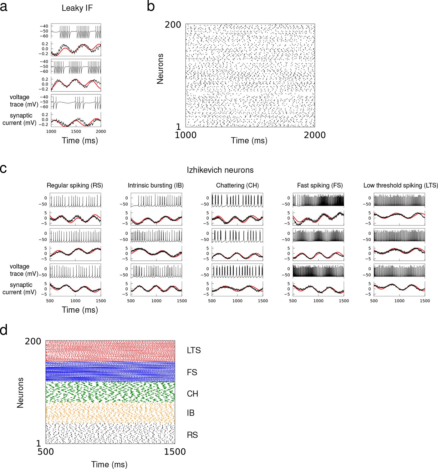
Learning recurrent dynamics with leaky integrate-and-fire and Izhikevich neuron models.

Synaptic drive of a network of spiking neurons were trained to follow 1000 ms long targets $f (t) = A s i n (2 π (t - T_{0}) / T_{1}) s i n (2 π (t - T_{0}) / T_{2})$ where $T_{0}, T_{1}$ and $T_{2}$ were selected uniformly from the interval [500 ms, 1000 ms]. (a) Network consisted of $N = 200$ leaky integrate-and-fire neuron models, whose membrane potential obeys ${\dot{v}}_{i} = - (v_{i} - I_{i}) / τ + u_{i}$ with a time constant $τ = 10$ ms; the neuron spikes when $v_{i}$ exceeds spike threshold $v_{t h r} = - 50$ mV then $v_{i}$ is reset to $v_{r e s} = - 65$ mV. Red curves show the target pattern and black curves show the voltage trace and synaptic drive of a trained network. (b) Spike rastergram of a trained leaky integrate-and-fire neuron network generating the synaptic drive patterns. (c) Network consisted of $N = 200$ Izhikevich neurons, whose dynamics are described by two equations ${\dot{v}}_{i} = 0.04 v_{i}^{2} + 5 v_{i} + 140 - w_{i} + I_{i} + u_{i}$ and ${\dot{w}}_{i} = a (b v_{i} - w_{i})$ ; the neuron spikes when $v_{i}$ exceeds 30 mV, then $v_{i}$ is reset to $c$ and $w_{i}$ is reset to $w_{i} + d$ . Neuron parameters $a, b, c$ and $d$ were selected as in the original study (Izhikevich, 2003) so that there were equal numbers of regular spiking, intrinsic bursting, chattering, fast spiking and low threshold spiking neurons. Synaptic current $u_{i}$ is modeled as in Equations 6 for all neuron models with synaptic decay time $τ_{s} = 30$ ms. Red curves show the target patterns and black curves show the voltage trace and synaptic drive of a trained network. (d) Spike rastergram of a trained Izhikevich neuron network showing the trained response of different cell types.

https://doi.org/10.7554/eLife.37124.008

Figure 3—figure supplement 3

Download asset Open asset

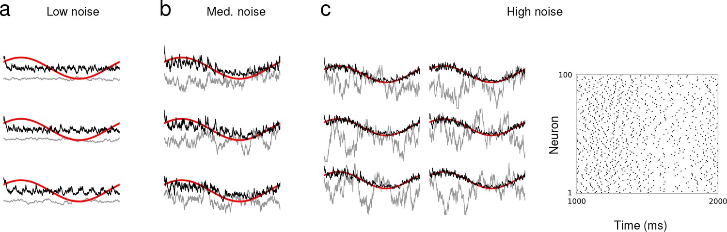
Synaptic drive of a network of neurons is trained to learn an identical sine wave while external noise generated independently from OU process is injected to individual neurons.

The same external noise (gray curves) is applied repeatedly during and after training. (a)-(b) The amplitude of external noise is varied from (a) low, (b) medium to (c) high. The target sine wave is shown in red and the synaptic drive of neurons are shown in black. The raster plot in (c) shows the ensemble of spike trains of a successfully trained network with strong external noise.

https://doi.org/10.7554/eLife.37124.009

Figure 4

Download asset Open asset

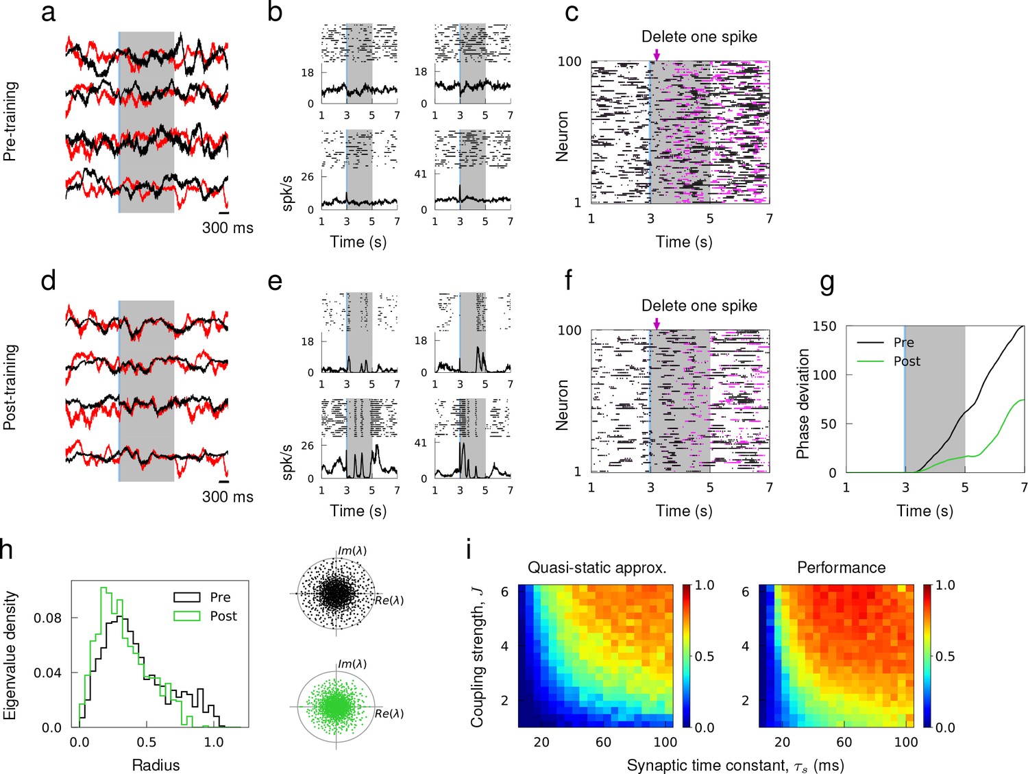
Learning innate activity in a network of excitatory and inhibitory neurons that respects Dale’s Law.

(a) Synaptic drive of sample neurons starting at random initial conditions in response to external stimulus prior to training. (b) Spike raster of sample neurons evoked by the same stimulus over multiple trials with random initial conditions. (c) Single spike perturbation of an untrained network. (d)-(f) Synaptic drive, multi-trial spiking response and single spike perturbation in a trained network. (g) The average phase deviation of theta neurons due to single spike perturbation. (h) Left, distribution of eigenvalues of the recurrent connectivity before and after training as a function their absolution values. Right, Eigenvalue spectrum of the recurrent connectivity; gray circle has unit radius. (i) The accuracy of quasi-static approximation in untrained networks and the performance of trained networks as a function of coupling strength J and synaptic time constant τ_s. Color bar shows the Pearson correlation between predicted and actual synaptic drive in untrained networks (left) and innate and actual synaptic drive in trained networks (right).

https://doi.org/10.7554/eLife.37124.010

Figure 5

Download asset Open asset

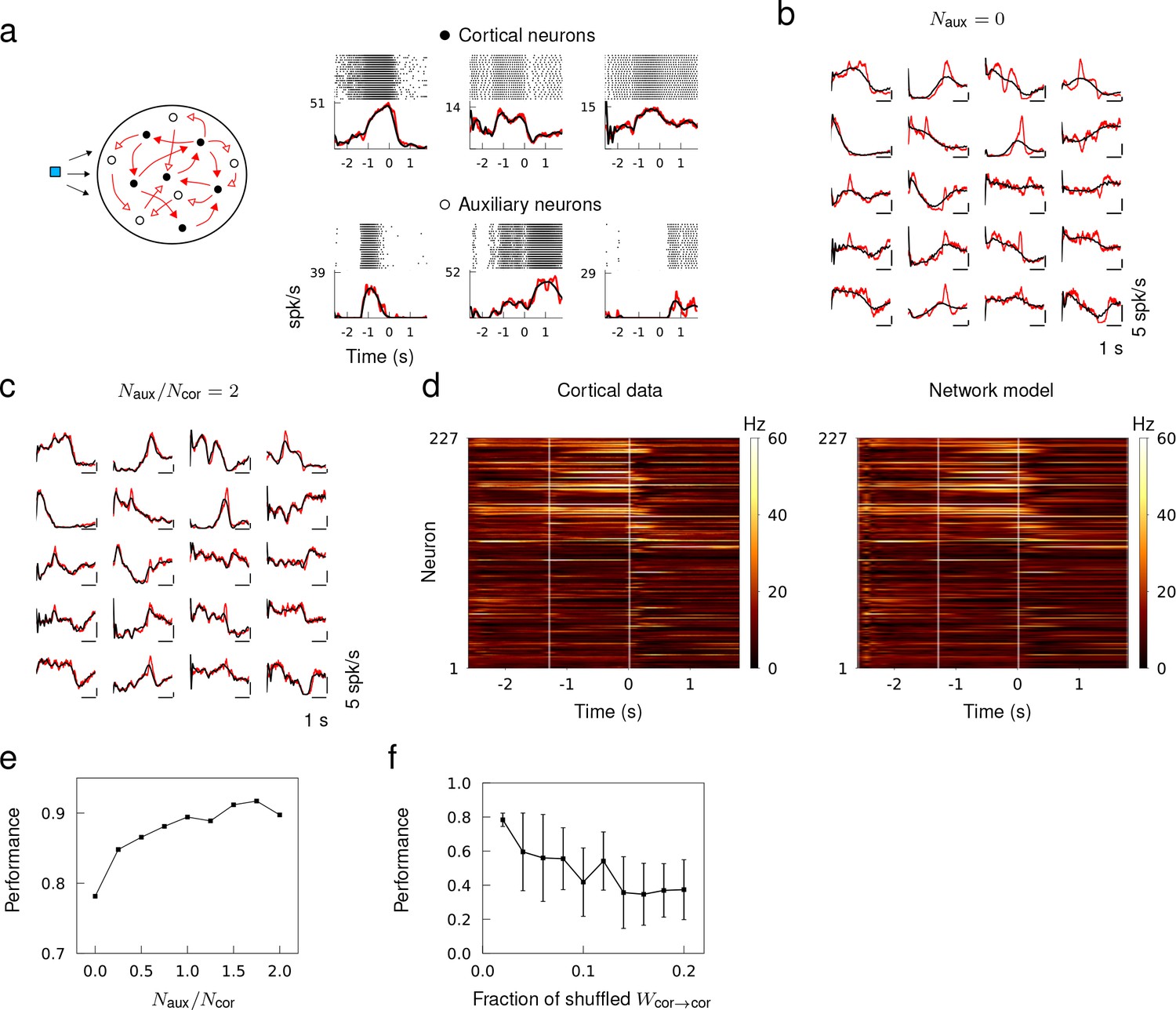
Generating in vivo spiking activity in a subnetwork of a recurrent network.

(a) Network schematic showing cortical (black) and auxiliary (white) neuron models trained to follow the spiking rate patterns of cortical neurons and target patterns derived from OU noise, respectively. Multi-trial spike sequences of sample cortical and auxiliary neurons in a successfully trained network. (b) Trial-averaged spiking rate of cortical neurons (red) and neuron models (black) when no auxiliary neurons are included. (c) Trial-averaged spiking rate of cortical and auxiliary neuron models when $N_{aux} = N_{aux} = 2$ . (c) Spiking rate of all the cortical neurons from the data (left) and the recurrent network model (right) trained with $N_{aux} = N_{cor} = 2$ . (e) The fit to cortical dynamics improves as the number of auxiliary neurons increases. (f) Random shuffling of synaptic connections between cortical neuron models degrades the fit to cortical data. Error bars show the standard deviation of results from 10 trials.

https://doi.org/10.7554/eLife.37124.011

Figure 6

Download asset Open asset

Sampling and tracking errors.

Synaptic drive was trained to learn 1 s long trajectories generated from OU noise with decay time $τ_{c}$ . (a) Performance of networks of size $N = 500$ as a function of synaptic decay time $τ_{s}$ and target decay time $τ_{c}$ . (b) Examples of trained networks whose responses show sampling error, tracking error, and successful learning. The target trajectories are identical and $τ_{c} = 100$ ms. (c) Inverted ‘U’-shaped curve as a function of synaptic decay time. Error bars show the s.d. of five trained networks of size $N = 500$ . (d) Inverted ‘U’-shaped curve for networks of sizes $N = 500$ and $1000$ for $τ_{c} = 100$ ms. (e) Network performance shown as a function of $τ_{s} / τ_{c}$ where the range of $τ_{s}$ is from 30 ms to 500 ms and the range of $τ_{c}$ is from 1ms to 500ms and $N = 1000$ . (f) Network performance shown as a function of $1 / \sqrt{N τ_{s}}$ where the range of $τ_{s}$ is from 1 ms to 30 ms, the range of $N$ is from 500 to 1000 and $τ_{c} = 100$ ms.

https://doi.org/10.7554/eLife.37124.012

Figure 7

Download asset Open asset

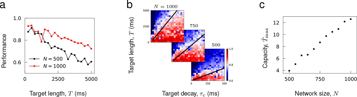
Capacity as a function of network size.

(a) Performance of trained networks as a function of target length $T$ for networks of size $N = 500$ and $1000$ . Target patterns were generated from OU noise with decay time $τ_{c} = 100$ ms. (b) Networks of fixed sizes trained on a range of target length and correlations. Color bar shows the Pearson correlation between target and actual synaptic drive. The black lines show the function $T_{m a x} = {\tilde{T}}_{m a x} τ_{c}$ where ${\tilde{T}}_{m a x}$ was fitted to minimize the least square error between the linear function and maximal target length $T_{m a x}$ that can be successfully learned at each $τ_{c}$ . (c) Learning capacity ${\tilde{T}}_{m a x}$ shown as a function of network size.

https://doi.org/10.7554/eLife.37124.013

Additional files

Transparent reporting form: https://doi.org/10.7554/eLife.37124.014
Download elife-37124-transrepform-v2.pdf

Download links

A two-part list of links to download the article, or parts of the article, in various formats.

Downloads (link to download the article as PDF)

Open citations (links to open the citations from this article in various online reference manager services)

Mendeley

Cite this article (links to download the citations from this article in formats compatible with various reference manager tools)

Christopher M Kim
Carson C Chow

(2018)

Learning recurrent dynamics in spiking networks

eLife 7:e37124.

https://doi.org/10.7554/eLife.37124

Sign up for email alerts

Privacy notice