Theoretical tool bridging cell polarities with development of robust morphologies
- University of Copenhagen, Denmark
Figures
Figure 1 with 1 supplement
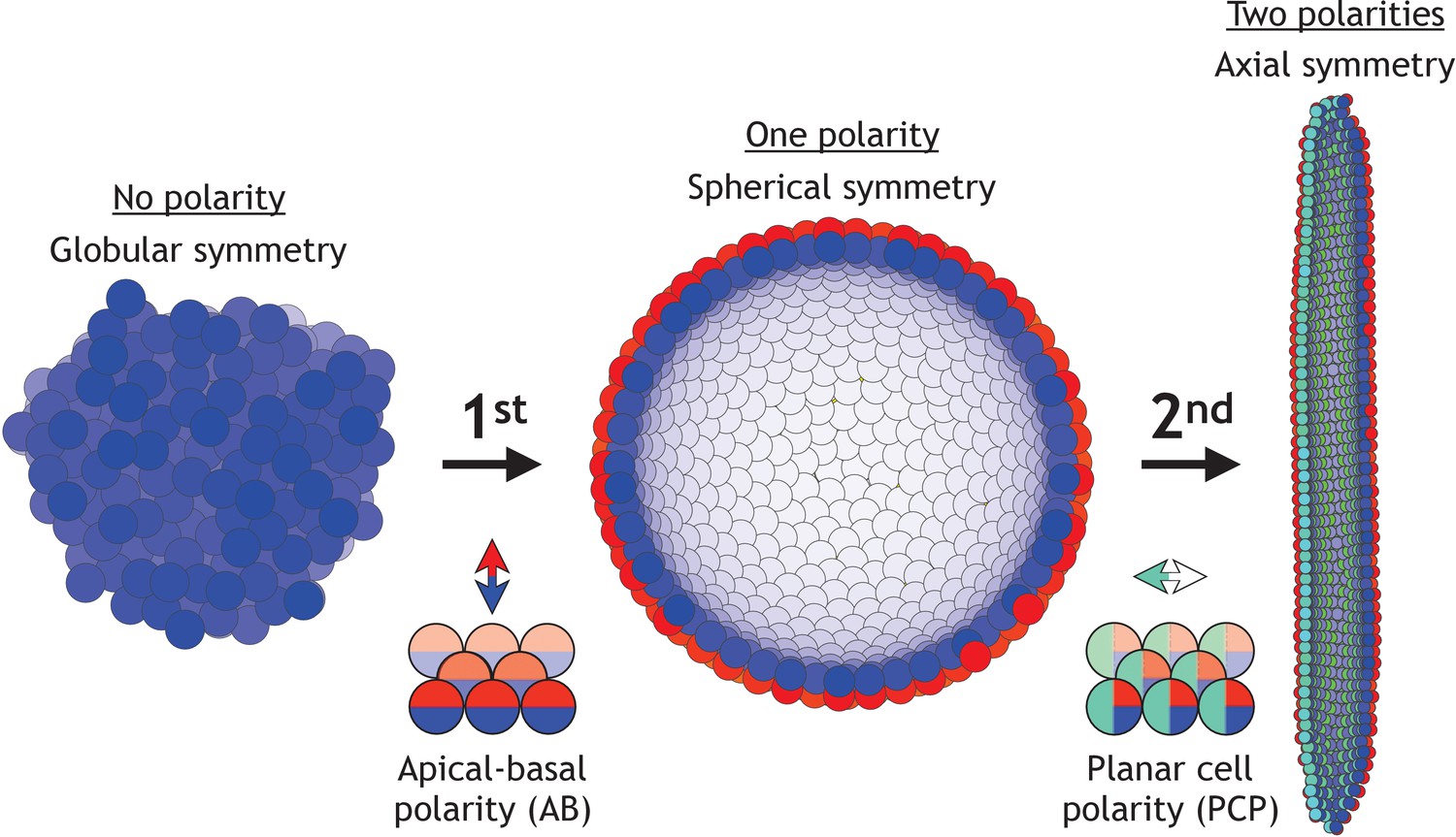
Two symmetry-breaking events, gain of apical-basal (AB) polarity and planar cell polarity (PCP), on cellular level coincide with the appearance of a rich set of morphologies.
Starting from an aggregate of non-polarized cells (globular symmetry), individual cells can gain AB polarity and form one or multiple lumens (spherical symmetry). Additional, gain of PCP allows for tube formation (axial symmetry). Complex morphologies can be formed by combining cells with none, one, or two polarities. In Figure 1—figure supplement 1, we schematically illustrate how existing models capture different elements of development.
Figure 1—figure supplement 1
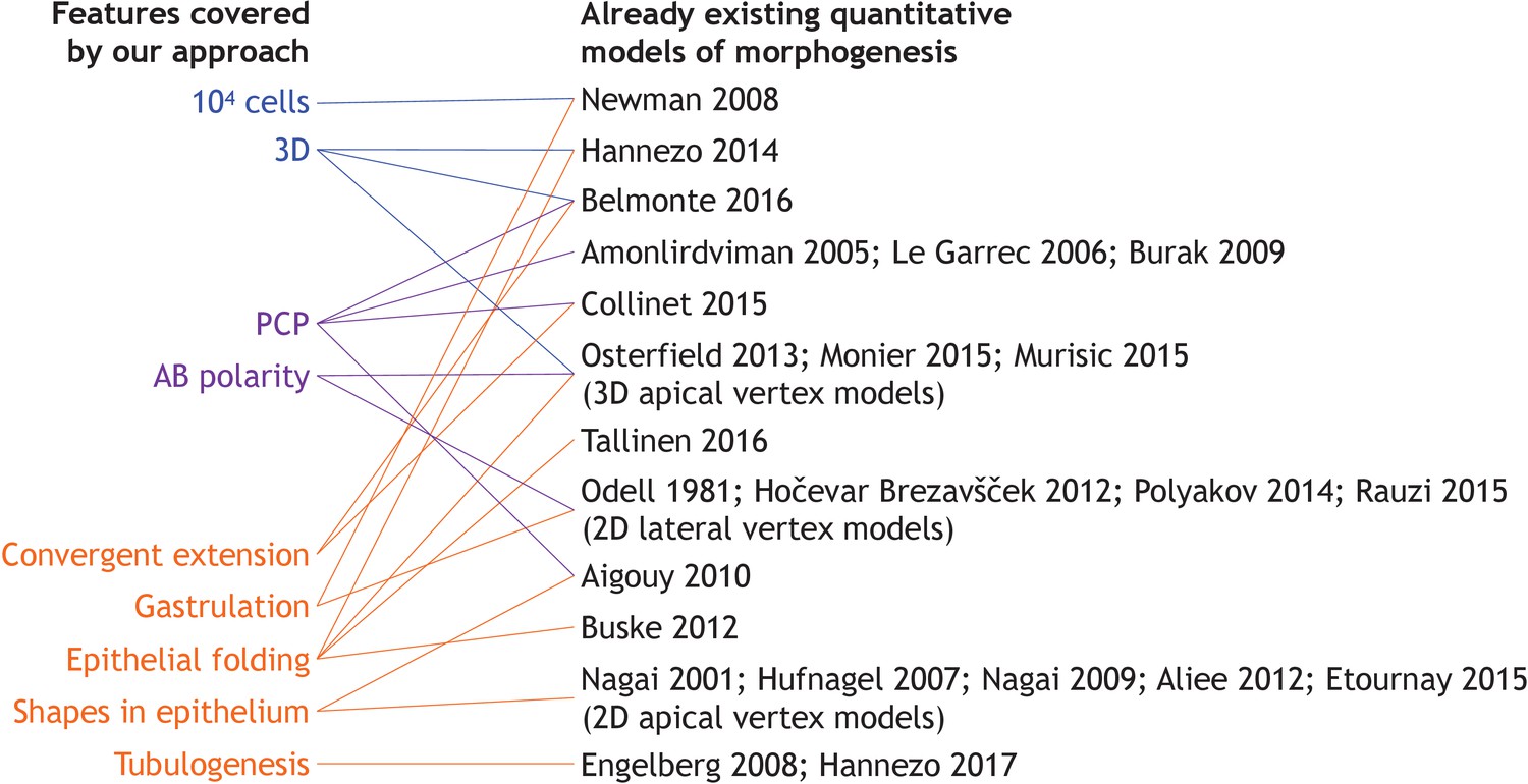
Overview of the existing literature on models addressing specific developmental events discussed in our work.
For more references on vertex models see Alt et al. (2017).
Figure 2 with 4 supplements
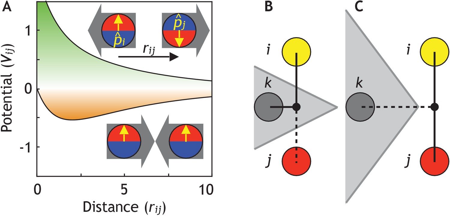
Cells are modeled as interacting particles with a polarity-dependent potential.
(A) Potential between two interacting cells with apical-basal polarity (see Equation 6). Cells repulse when polarities are antiparallel (top/green part) and attract when they are parallel (orange/bottom part). (B–C) Two cells interact only if no other cells block the line of sight between them. (B) Cell i and j do not interact if ij’s midpoint (black dot) is inside of the Voronoi diagram for cell k (shaded in grey). (C) Cell i and j interact because cell k is further away than the distance ij/2 and ij’s midpoint therefore lie outside of cell k’s Voronoi diagram. In the related Figure 2—figure supplement 1A–D, we test the sensitivity of our model to the details of the potential and neighborhood assignments. In Figure 2—figure supplement 2, we relate changes in cell shapes to the model components, and in Figure 2—figure supplement 3 (Figure 2—video 1), we illustrate how altering polarity affects the dynamics of the systems with two and six cells.
Figure 2—figure supplement 1

Dependence on the shape of the physical potential, the interaction partners, and noise.
(A) Applying the neighborhood function shown in Figure 2, but changing the shape of the potential to the short-range potential written in Equation 2, the system unfolds and reaches a stable state (η = 10−4). (B) Full Voronoi interactions with a cut-off does also lead to a stable state, although a few cells might lose interaction with the majority of cells (cut-off at three shown). (C) However, a simple cut-off (and no Voronoi) does not result in stable morphologies but broken sheets on top of each other (cut-off at 2.5 shown). (D) The same happens, when all cells always interact with their six nearest neighbors. (E) With changed initial conditions compared to Figure 3, the system reaches a different stable state with low noise (η = 10−4). (F) However, this is comparable to the state obtained under high noise (η = 10−1). (G) Increasing the noise in (E) at time log(t) = 4 from η = 10−4 to η = 10−1, it results in fewer permutations than having high noise during the entire simulation which is shown in (F). The lower-case letters in (E–G) point at macroscopic features (a–h on one side in blue and r–u on the other side in red). The initial positions and polarities are identical for all seven simulations.
Figure 2—figure supplement 2
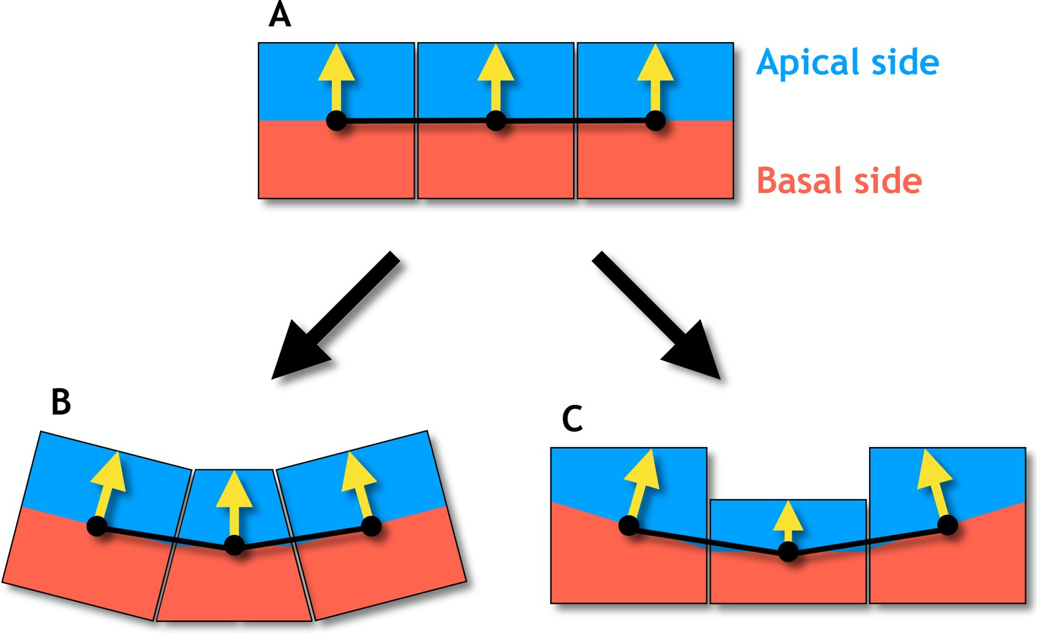
Changes in cell shapes may reorient apical-basal (AB) polarity.
(A) In an epithelial sheet AB polarity (yellow arrows) points perpendicular to the sheet. (B) Regulated changes in planar cell polarity can reorient the AB polarities in neighboring cells by apical constriction (narrowing of the apical side) giving rise to a central bottle cell. (C) If the AB polarity is shortened, the neighboring cells will reorient in a similar way. These results are obtained under the assumption that the AB polarity tends to orient perpendicular to the distance vectors (black lines) connecting cells’ centers of masses (black dots) which are central to the model presented.
Figure 2—figure supplement 3
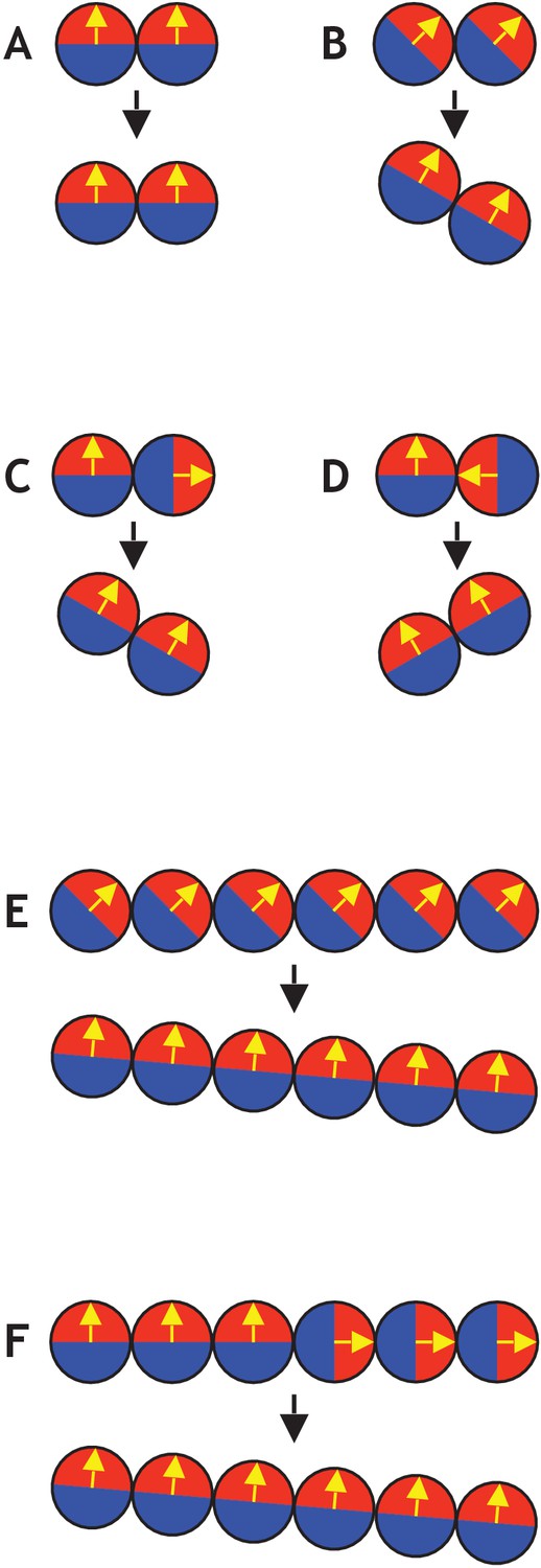
Examples of simple systems consisting of only two or six cells (see also Figure 2—video 1).
(A) Two cells initially aligned do not result in any movement. (B) If both cells’ polarities are 45 degrees to the plane, the axis of position becomes tilted by 30 degrees. (C) If one cell points away from another in a two-cell system, it tilts the axis of position. (D) Similar to (C), if one cell points towards another, it tilts in the other direction. (E) Similar to (B), but with six cells instead of two. In this case, the final axis of position is only tilted by five degrees compared to the initial axis. (F) Similar to (C) and (E), with three cells pointing up and three cells pointing to the right. This also gives a final axis of position that is tilted by five degrees compared to the initial axis.
Figure 2—video 1
Dynamics for two and six interacting cells.
(A) No movement occurs if the polarities are perfectly aligned and the distance between the cells is at steady state. (B) If both cells initially have their polarities 45 degrees to the axis of position, then both cells rotate slightly, and at the final stage the axis of position has been rotated by 30 degrees. (C) Initializing one cell with polarity up and another cell with polarity to the right results in substantial rotation of the latter cell and less rotation of the first cell. Finally, the cells reach steady state positioning each other on a tilted axis. (D) Opposite (C). One cell has polarity up while another cell points left. This results in an axis that is tilted to the left. (E) Similar to (B), but with six cells having their polarities initially 45 degrees to the axis of position. In this case, the outermost cells move the most and rotate slower than the four inner cells. Finally, resulting in an only slightly tilted plane. (F) Similar to (C) and (E). On the left three cells point initially up while on the right three cells point initially to the right. In this case, the three cells on the left almost do not rotate and move at all while the three cells on the right rotate and move substantially. In all panels, there is no noise, η = 0, and dt = 0.1 (see also Figure 2—figure supplement 3).
Figure 3 with 3 supplements

Development of 8000 cells from a compact aggregate starting at time 0.
(A) Cells are assigned random apical-basal polarity directions and attract each other through polar interactions (see Equation 6). (A–D) Cross-section of the system at different time points with red and blue marking two opposite sides of the polar cells. Cells closest to the viewer are marked red/blue, whereas cells furthest away are yellow/white. (E) Full system at the time point shown in (D). (F) Development of the number of neighbors per cell (red) and the energy per cell (blue), as defined by the potential between neighbor cells in Figure 2. Dark colors show the mean over all cells while light-shaded regions show the cell–cell variations. The yellow dot marks the energy for a hollow sphere with the same number of cells. See Figure 3—video 1 for full time series. In Figure 2—figure supplement 1E–G and Figure 3—figure supplement 1, we study how the final morphology depends on noise. In Figure 3—figure supplement 2, we show how the outer surface self-seals, and that the shape is maintained when cells divide.
Figure 3—figure supplement 1
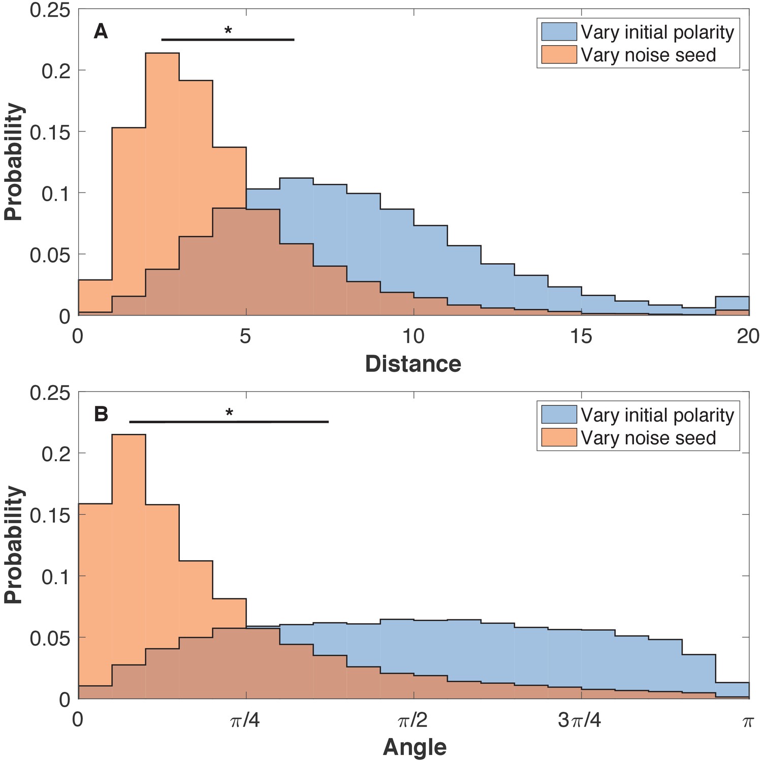
The final shapes are more sensitive to initial polarities than to noise.
(A) The pairwise distance between cells for three systems with identical initial polarities but different noise and three systems with identical noise but different initial polarities. (B) For the same set of aggregates, the angle between the pairwise polarities is calculated. The initial positions are the same for all systems. Each system has 8000 cells. Cells are pairs if they were initiated with identical position. Here, the noise level is η = 10−4. Two-sample Kolmogorov-Smirnov tests showed p < 0.001 statistical significance (marked by *). Comparing noise levels give similar results as comparing noise seed. The initial polarities are random like in Figure 3.
Figure 3—figure supplement 2
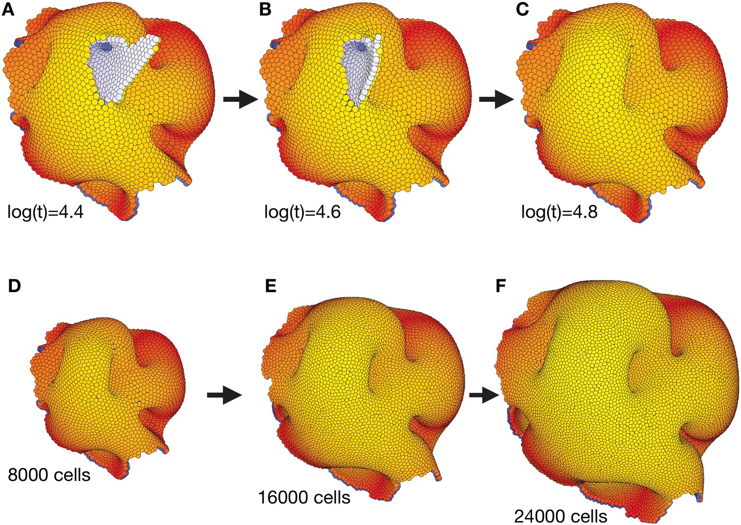
The complex morphology in Figure 3 self-seals and is robust to overall system growth.
(A–C) Self-sealing properties of polarized cell surfaces when close to a final stable state in Figure 3. While the internal morphology remains the same from time log(t) = 3.6 (Figure 3C–D and Figure 3—video 1), some of the outer surfaces subsequently reorganize to form a less disrupted torus-like structure with multiple handles. (D–F) The final structure in (C) (and Figure 3D–E together with the end of Figure 3—video 1) is robust to cell divisions. For every 10th time step, we select a cell by random, and let it divide in an arbitrary direction. We see that the overall shape of the structure is maintained, and that it expands equally in all directions.
Figure 3—video 1
An aggregate of 8000 cells with initial random polarities unfolds into a stable complex morphology.
During the simulation, the polarities and positions are updated dynamically with equal speed and noise (dt = 0.1 and η = 10−3). There is no planar cell polarity (λ1 = 1 and λ2 = λ3 = 0). (A) The entire system unfolds, and we notice that the outer surface reaches equilibrium state later than the internal morphology (see also Figure 3—figure supplement 2). (B) Cross-section of the system at y = 0. (C) Same as (B) but viewed from an angle slightly above and from a side. The color scheme is as described in Figure 3.
Figure 4 with 1 supplement
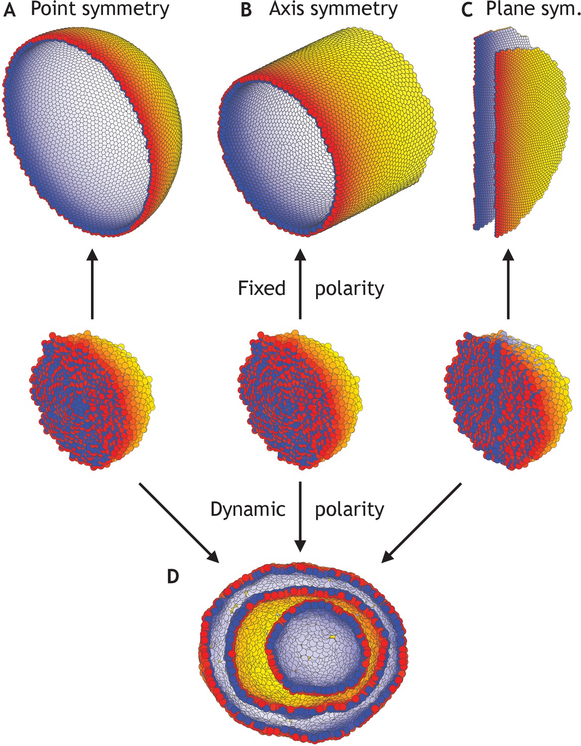
Different morphologies can be obtained by varying boundary conditions (Figure 4—video 1).
(A) A hollow sphere emerges if polarities are fixed and initially point radially out from the center of mass. (B) A hollow tube is obtained if polarities point radially out from a central axis. (C) Two flat planes pointing in opposite directions are obtained if polarities point away from a central plane. (D) For all three initial conditions (A–C), if the polarities are allowed to change dynamically and the noise is high (η = 100 compared to η = 10−1 in A–C), the resulting shape consists of three nested ‘Russian doll’-like hollow spheres that will never merge due to opposing polarities. In contrast to the random initial condition in Figure 3, the initial conditions in (D) are symmetric.
Figure 4—video 1
Dynamics when the polarities have restricted orientations.
In all three simulations, an aggregate consisting of 8000 cells develops into three simple morphologies due to polarities being fixed in different directions. (A) One big lumen forms when the polarities are restricted to point radially out from the center-of-mass. At an early stage, a small lumen forms around the center-of-mass. Later the shell transiently consists of multiple cell layers. However, in the end, these layers merge into a single cell layer (Figure 4A). (B) A tube emerges when the polarities are restricted to point away from a central axis. Similar to (A) a small tube appears at an early stage deep inside the aggregate, and transiently it contains multiple cell layers (Figure 4B). (C) Finally, two opposing planes form when the polarities are restricted to orient away from a central plane. This develops in a similar way as (A) and (B) without rotating any cells (Figure 4C). Throughout all three simulations, dt = 0.1 and the noise parameter η = 0.1.
Figure 5 with 2 supplements
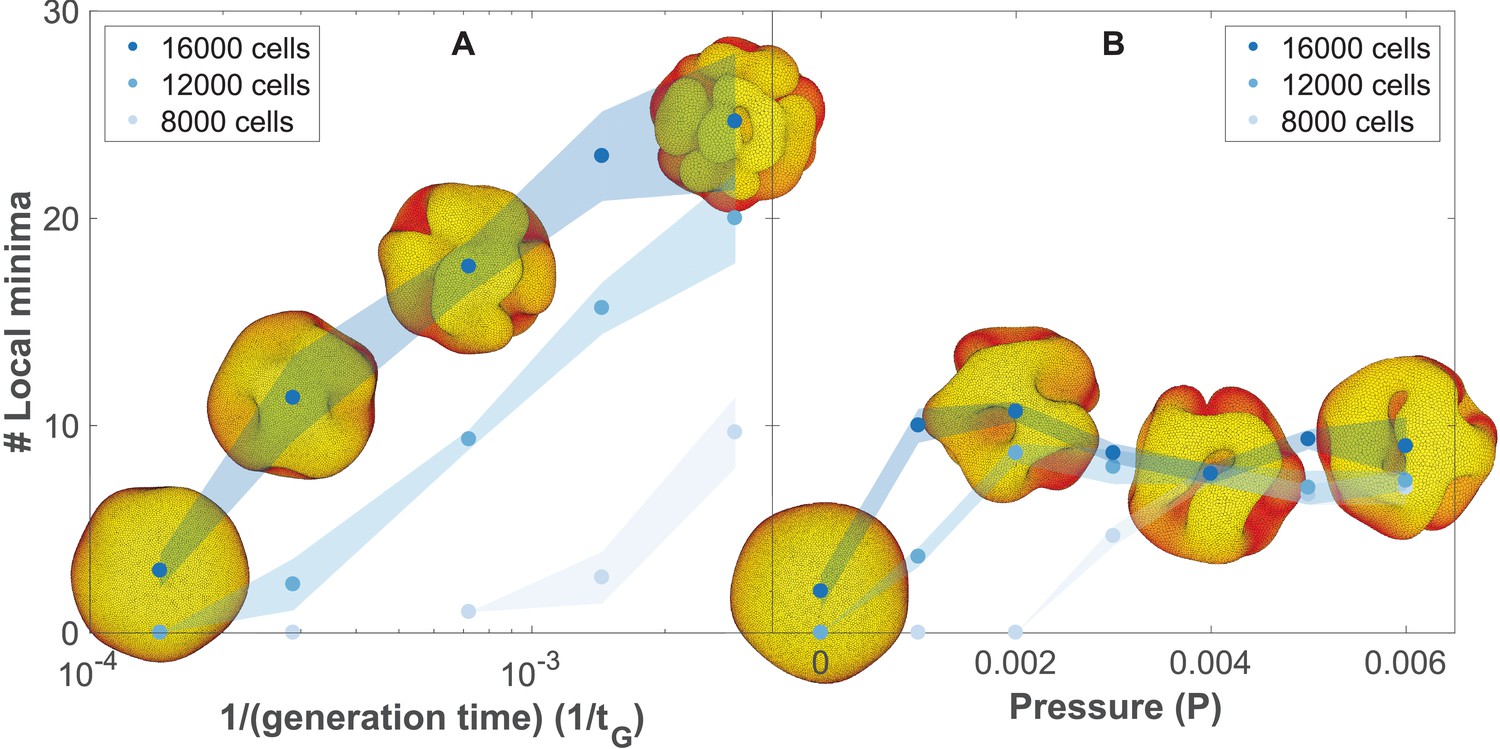
The number of complex folds in a growing organoid depends on the generation time and the pressure from the surrounding medium (Figure 5—video 1).
(A) Number of local minima as a function of 1/(generation time), tG−1. In silico organoids grow from 200 cells up to 8000, 12,000, or 16,000 cells with different generation times and no outer pressure. (B) Number of local minima as a function of pressure, P. In silico organoids grow to the same size with the same 1/(generation time), tG−1 = 1.4⋅10−4 but different outer pressure. The images illustrate the 16,000 cells stage. Blue dots mark the average, while light shaded regions show the SEM based on triplicates. See also Figure 5—figure supplement 1 for additional measurements on the differences between rapid growth and pressure.
Figure 5—figure supplement 1

Organoids grown under external pressure have deeper and longer folds compared to organoids grown with rapid cell proliferation.
To quantify the folds, we fill the surface of the organoids with 'water' until halfway between the maximum and minimum radius of the system. Then we measure the relative depth and circumference of these ‘lakes’. (A–C) Deepest point of the ‘lakes’ (folds) relative to the water level. The probability of having a lake at a given depth is normalized to the number of ‘lakes’. (D–F) Length of the ‘lakes’ relative to the entire circumference at this same level. Length of a lake is defined from the angle between the two cells at lake shore that are the furthest away from each other. Pressure and 1/(generation time) increase from upper to lower panels. Two-sample Kolmogorov-Smirnov tests showed p < 0.001 statistical significance (marked by *). The shown histograms are for the 16,000 cell stage, which compares to the dark blue line in Figure 5.
Figure 5—video 1
In silico organoids grown from 200 up to 16,000 cells.
(A) Increasingly many near-surface folds emerge when the organoid is grown with rapid cell proliferation (tG−1 = 7⋅10−3, p = 0, Figure 5A). (B) Number of deep folds saturates when the organoid is grown slowly under resistance from matrigel (tG−1 = 1.4⋅10−4, p = 0.006, Figure 5B). Videos at the top illustrate the entire system, while the those at the bottom shows a cross-section of the system. Throughout, all organoid simulations in Figure 5 including the ones shown in this video, η = 10−4 and dt is the minimum of 0.2 and one fifth of the time to the next consecutive division in the system.
Figure 6 with 4 supplements
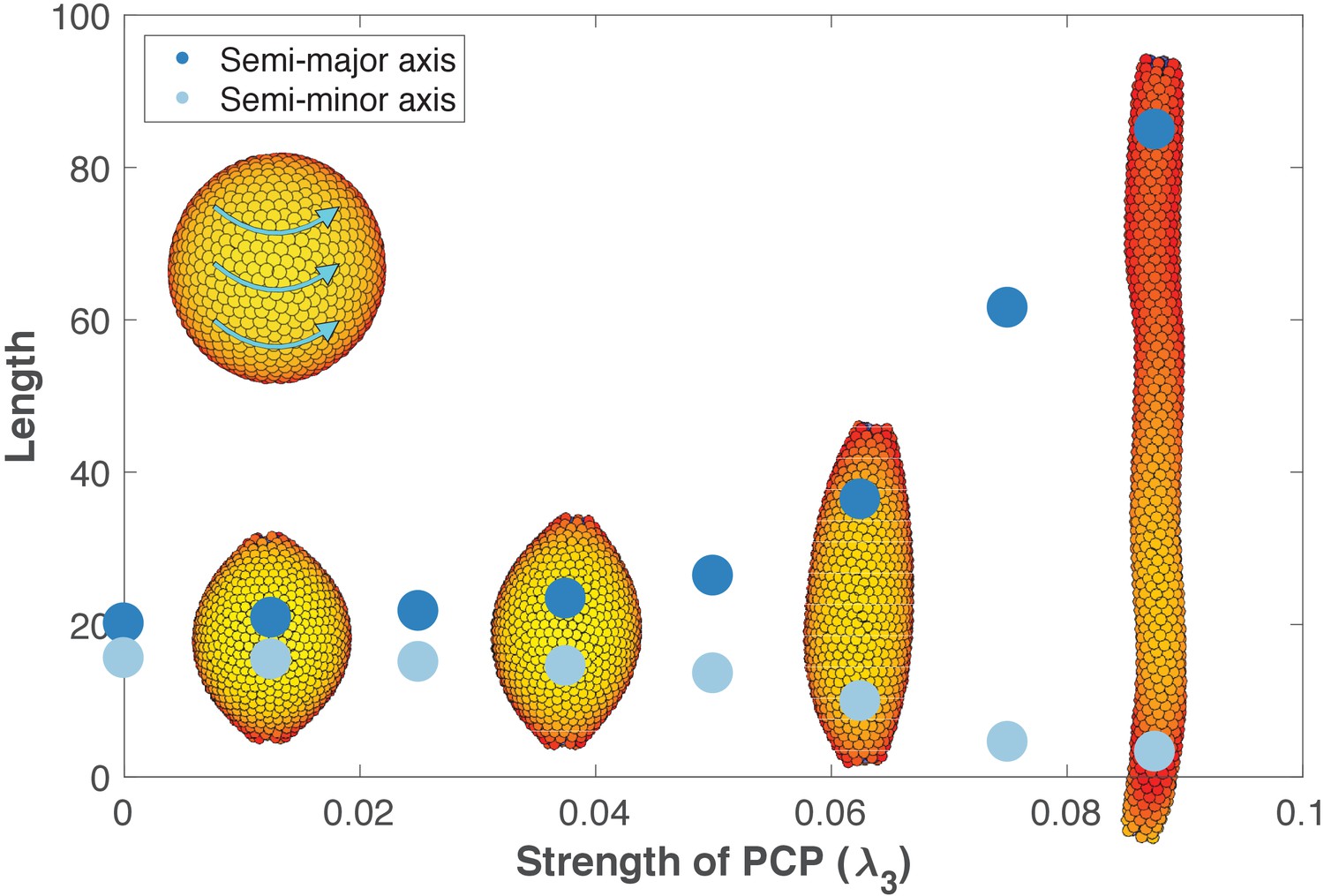
The length and width of tubes are set by the strength of planar cell polarity (PCP, λ3).
For each value of λ3, we initialize 1000 cells on a hollow sphere with PCP whirling around an internal axis (PCP orientation marked by cyan arrows in the top-left inset). Semi-major axis (dark blue) and semi-minor axis (light blue) are measured at the final stage (Materials and methods). Images show the final state. Throughout the figure, λ2 = 0.5 and λ1 = 1 - λ2 - λ3. The animated evolution from sphere to tube is shown in Figure 6—video 1. See also Figure 6—figure supplement 1 where we show that tubes also form when we disable the direct influence of PCP on apical-basal polarity, and Figure 6—figure supplement 2 where we vary the degree of PCP along the axis of the tube. In Figure 6—figure supplement 3, we show that cell intercalations result in experimentally reported T1 neighbor exchanges during convergent extension.
Figure 6—figure supplement 1
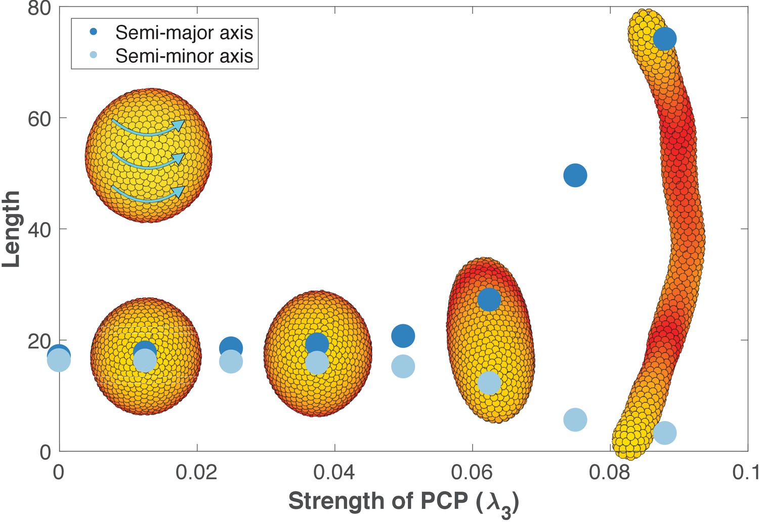
Removing the influence of planar cell polarity (PCP) on apical-basal (AB) polarity.
This figure is identical to Figure 6 with the only difference that now λ2 = 0 when updating AB polarity (λ2 = 0.5 when updating position and PCP as in Figure 6). The strength of PCP (λ3) is defined as shown along the x-axis. λ1 = 1 - λ2 - λ3 for updating position and PCP, and for updating AB polarity λ1 = 0.5 - λ3. This way λ1 and λ3 are the same for position, AB polarity, and PCP, and the only change is the value of λ2. The final tubes are slightly wider and shorter compared to Figure 6 since the tips become more rounded when PCP does not affect AB polarity. Throughout, all the simulations in this figure, dt = 0.2 and the noise parameter η = 5⋅10−5.
Figure 6—figure supplement 2
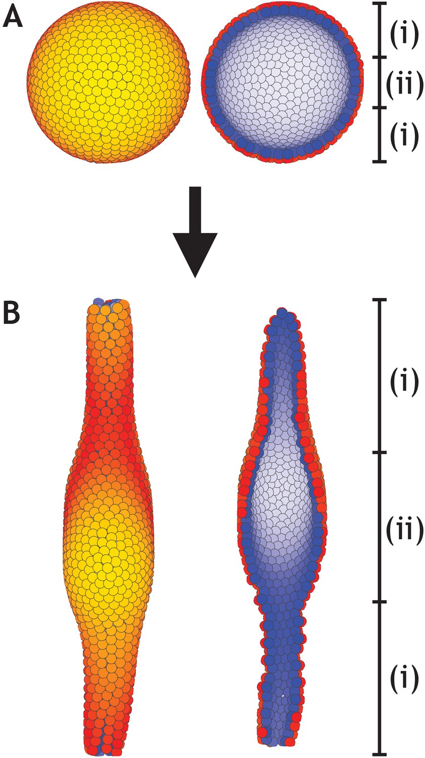
A lumen forms inside a developing tube in areas that lack planar cell polarity (PCP).
(A) Similar to Figure 6, a hollow sphere of cells is initialized. However, in this example only cells inside zone (i) have PCP while cells inside zone (ii) do not have PCP. (B) At the final stage, an elongated tube with a central lumen has formed. Images to the left show the entire system while images to the right show a cross-section. Cells inside zone (i) develop with λ1 = 0.41, λ2 = 0.5, and λ3 = 0.09 while cells inside zone (ii) develop with λ1 = 1, and λ2 = λ3 = 0. The central third of the 1000 cells in the system belong to zone (ii). Throughout, the simulation dt = 0.1 and η = 10−4.
Figure 6—figure supplement 3
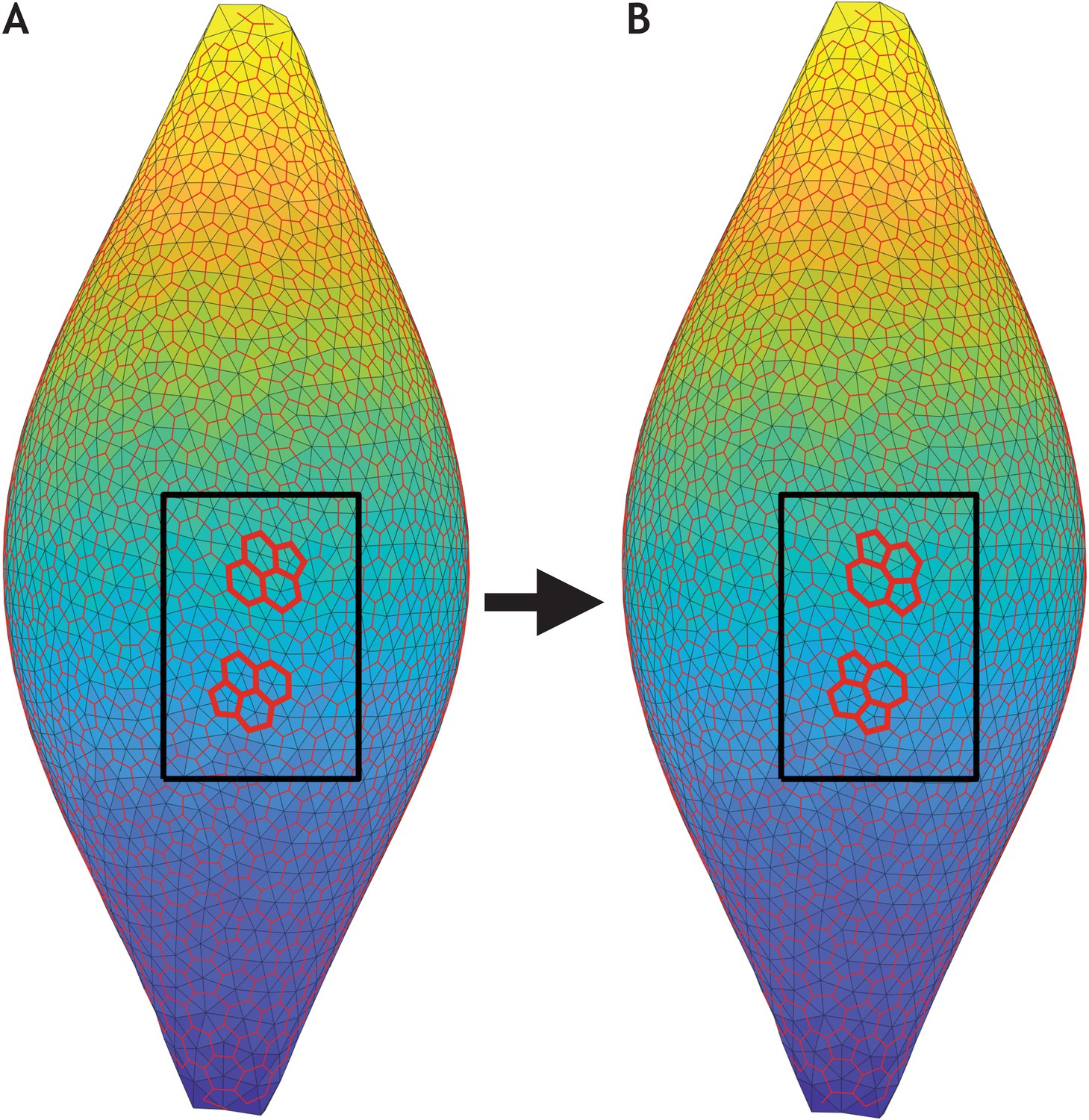
T1 exchanges occur during sphere–tube transition.
Two consecutive time frames of the most extreme scenario in Figure 6 (λ1 = 0.41, λ2 = 0.5, and λ3 = 0.09, see also Figure 6—video 1). (A) Snapshot of the entire system at time t = 1259.0. (B) Snapshot slightly later at time t = 1288.3. In both panels, the cell centers (light grey vertices) are triangulated (light grey edges). Triangle centers (red vertices) are calculated in order to get an approximate location of the cell borders (red edges). Inside the black box, two T1 exchanges (bold red lines) are highlighted.
Figure 6—video 1
Model of tubulogenesis.
Planar cell polarity (PCP) is tunred on in a spherical lumen consisting of 1000 cells with apical-basal polarity pointing radially out. In equilibrium, PCP will curl around an internal axis. Depending on the relative strength of the polarities the sphere will elongate and transform to a tube with a given length and width. This video illustrates the most extreme scenario in Figure 6 (λ1 = 0.41, λ2 = 0.5, and λ3 = 0.09). The left panel shows the entire system while the right panel shows a cross-section of the system. Throughout all simulations in Figure 6 including the one presented in this video, dt = 0.2 and η = 5⋅10−5. The color scheme is as described in Figure 3.
Figure 7 with 2 supplements
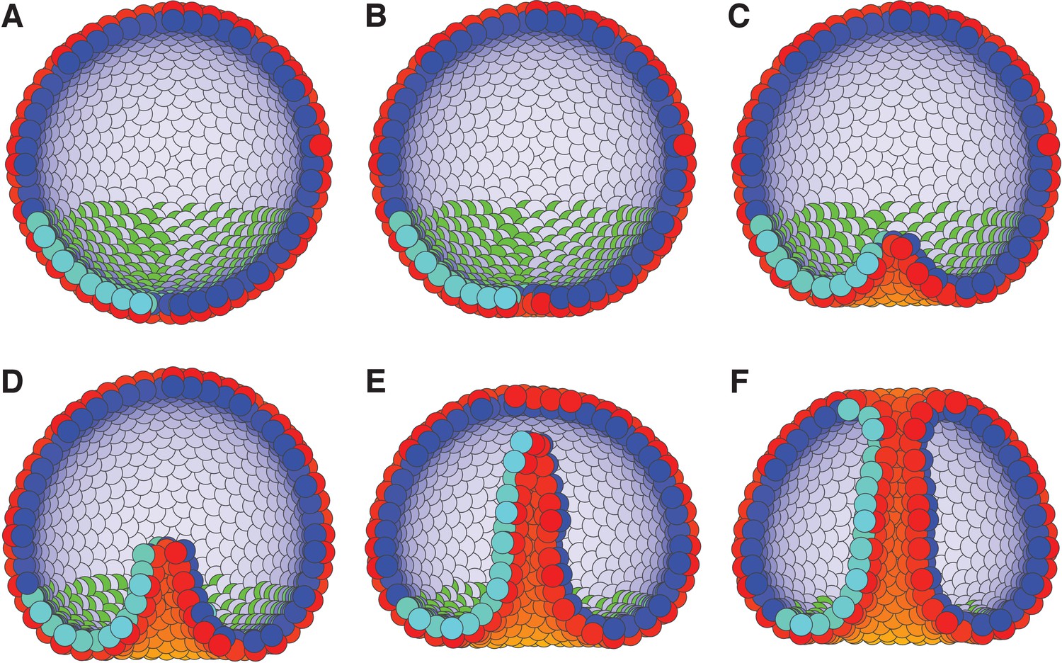
External constraints on apical-basal (AB) polarity and planar cell polarity (PCP) can initiate invagination and drive gastrulation in sea urchin.
(A) The lower third of the cells in a blastula with AB polarity (apical is blue–white, basal is red–orange) pointing radially out acquire PCP (cyan–green) in apical plane pointing around the anterior-posterior (top-bottom) axis (as in the inset to Figure 6). (B) Flattening of the blastula and (C) invagination occur due to external force reorienting AB polarity (Materials and methods). (D–E) Tube elongation is due to PCP-driven convergent extension and (F) merging with the top of the blastula happens when the tube approaches the top. Throughout the simulation, λ1 = 0.5, λ2 = 0.4, and λ3 = 0.1 for the lower cells while the top cells have λ1 = 1 and λ2 = λ3 = 0. For full time dynamics see Figure 7—video 1. In Figure 7—figure supplement 1, we consider alternative scenarios of sea urchin gastrulation and and neurulation.
Figure 7—figure supplement 1
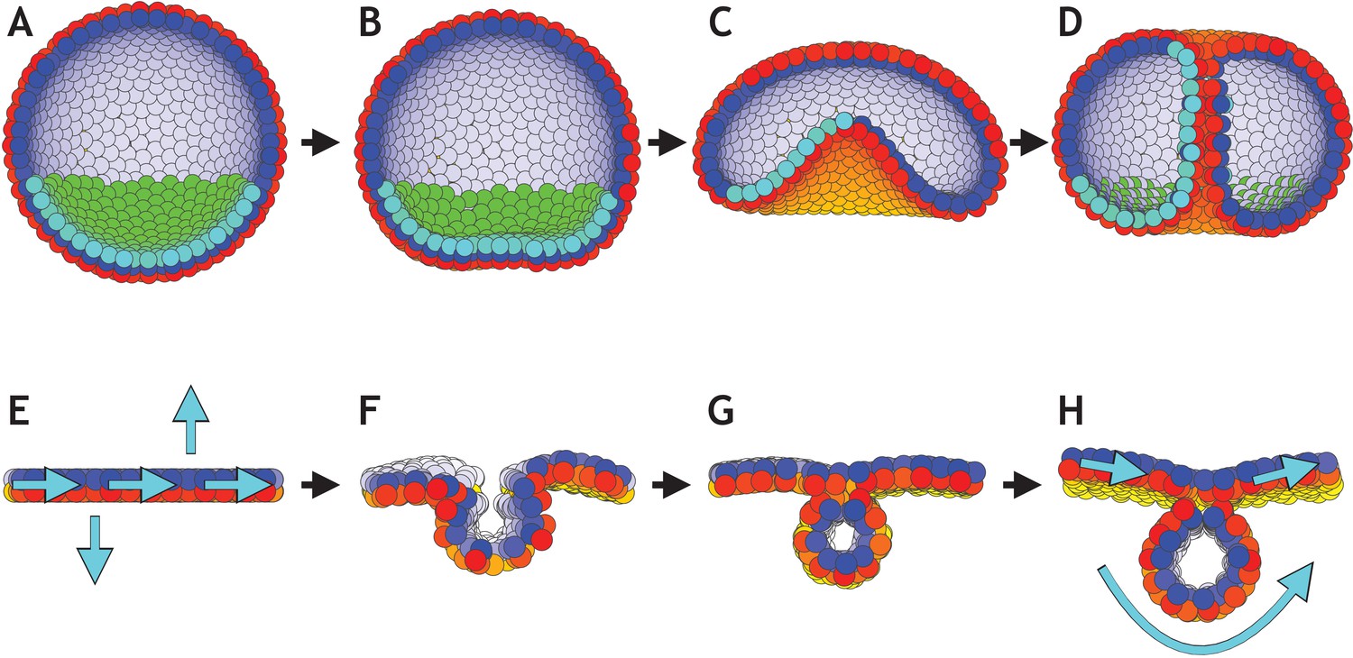
Directed changes in the direction of planar cell polarity (PCP) may drive invagination in gastrulation and neurulation.
(A–D) Gastrulation in sea urchin modeled without the apical constriction in Figure 7. (A) The lower third of the cells in the blastula acquire PCP (cyan–green) pointing opposite to the apical-basal (AB) polarity (red–yellow). (B) Flattening of the blastula and invagination occur if direction of PCP is maintained for some time. During this initial phase λ2 = 0.1, and there is no convergent extension (λ3 = 0). (C) In the final phase, we increase λ2 to 0.4 and turn on λ3 = 0.1. With this, we let PCP relax so it curls around the bottom, and allow it to change dynamically in time. (D) As a result, tube narrows and elongates, until it finally connects and merges with the top. (E–H) Initial conditions on PCP enable neural plate bending and neural tube closure. (E) Starting with 1000 cells on a plane with AB polarity, we induce PCP along the plane together with two rows where the PCP points parallel and antiparallel to AB polarity (shown with cyan arrows). Here, we simulate the neural plate (cells in the middle, between the two rows with constrained PCP) surrounded by the epidermis (the rest of the cells). The two rows of cells with PCP pointing out of epithelial plane correspond to the cells at the dorsolateral hinge points next to the neural plate (epidermis boundaries). In chick, spinal neural tube can close with only these two hinge points (Nikolopoulou et al., 2017). The bending is driven by apical constriction and PCP is essential for bending, convergent extension and closure. (F) This enables neural plate bending and formation of the neural groove. (G) Continuing the simulation leads to contact of the two sides of the neural plate and hereby neural tube closure. (H) Finally, the system stabilizes with the neural plate on top of the neural tube. Comparing the initial stage to the final stage, the overall direction of PCP in the plate is conserved while in the tube PCP goes around an internal axis. For this simulation, we set λ2 = 0.5 and λ3 = 0. Turning on convergent extension (λ3) at the final stage will allow for elongating the system along the axis going through the tube and narrowing it in another direction. The concept is similar to gastrulation in Drosophila. In both simulations, sea urchin and neurulation, dt = 0.3. In sea urchin (A–D), the noise parameter η = 3.3⋅10−5, and in neurulation (E–H), η = 3.3⋅10−2.
Figure 7—video 1
Model of sea urchin gastrulation.
Starting from a hollow sphere of 1000 cells with apical-basal polarity pointing radially out. The bottom flattens and invaginates by applying an external force to mimic apical constriction (see Materials and methods), and by giving a fraction of cells planar cell polarity pointing around the sphere. The tube forms, elongates, and connects with the upper part of the blastula. Throughout the simulation, dt = 0.1 and η = 10−4. For more details see the caption to Figure 7. Panels are similar to Figure 6—video 1. The color scheme is as described in Figure 3 and Figure 7.
Author response image 1
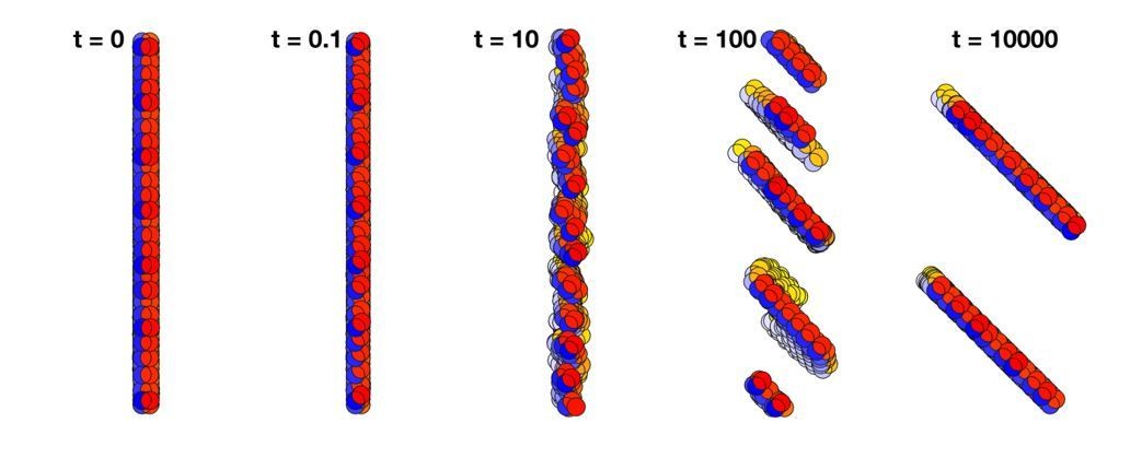
Changing the polarized direction of a plane of cells does not rotate the plane as a whole but breaks it into smaller planes.
Time t = 0 shows a plane consisting of 500 cells with AB polarity pointing to the right. At time t = 0.1, the direction of the polarity is shifted by 45 degrees. Since the polarity is fixed in time, the planes break into smaller pieces, and at time 104 they have merged into two planes that are separated by several cell diameters.
Author response image 2
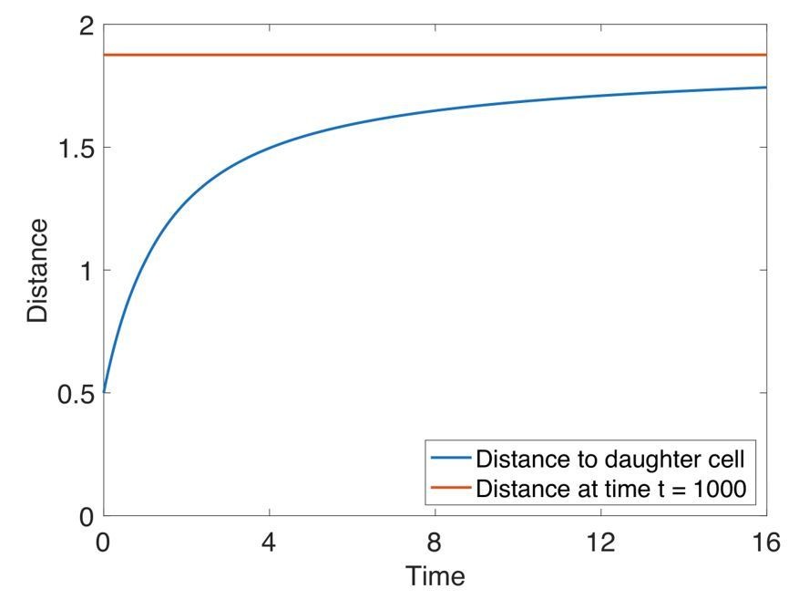
At cell division, the daughter cell equilibrates by half a cell radius in one time unit, which is of order 1/1000 the generation time.
Here, we show how a new cell (in blue) reaches equilibrium (in red). Cell division happens at time 0. At time 5, the next consecutive division happens in the system (not shown). The systems consists of 200 cells placed on a hollow sphere which is the initial condition in our organoid simulations (Figure 5). A new cell is introduced half a cell radius in a random direction away from the mother cell. The red line is the mean distance from the mother cell to all it’s neighbor cells at t = 1000. The generation time is intermediate (Figure 5A).
Additional files
-
Source code 1
MATLAB script.
- https://doi.org/10.7554/eLife.38407.027
-
Transparent reporting form
- https://doi.org/10.7554/eLife.38407.028
Download links
A two-part list of links to download the article, or parts of the article, in various formats.
Downloads (link to download the article as PDF)
Open citations (links to open the citations from this article in various online reference manager services)
Cite this article (links to download the citations from this article in formats compatible with various reference manager tools)
Theoretical tool bridging cell polarities with development of robust morphologies
eLife 7:e38407.
https://doi.org/10.7554/eLife.38407


