Recalibrating timing behavior via expected covariance between temporal cues
Figures
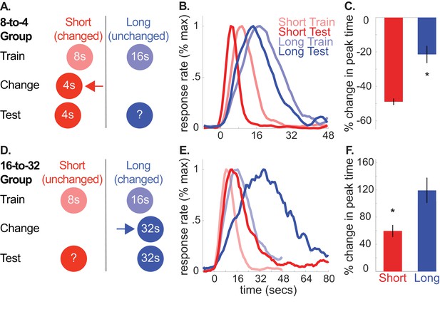
A and D depict the general design used for the 8-to-4 (n = 10) and 16-to-32 (n = 10) groups, respectively.
(B) and (E) show average normalized response rate during probe trials during initial training and testing for the 8-to-4 and 16-to-32 groups, respectively. For presentation, each curve was normalized by the maximum value and smoothed over a 6-bin window. (C) and (F) show percent-change in peak time during testing (±SEM), relative to initial training for the 8-to-4 and 16-to-32 groups, respectively. Stars indicate significance (p<0.05).
-
Figure 1—source data 1
Data used to generate Figure 1.
- https://doi.org/10.7554/eLife.38790.010
-
Figure 1—source data 2
Table showing percent change in peak, start, and stop times (+/- SEM) for the unchanged cue across all experiments.
Stars indicate significance under an alpha level of .05. Tildes indicate marginally significant effects (p < .1).
- https://doi.org/10.7554/eLife.38790.009

Raw probe trial response rates during training and testing for all experiments.
A shows responding in the 8-to-4 (left) and 16-to-32 (right) groups of Experiment 1. B shows responding in the no-change control group of Experiment 1. (C) shows responding in the 8-to-12 group of Experiment 2. (D) shows responding for the change (left) and no-change (right) groups of Experiment 3. (E) shows responding in the correlated (left) and uncorrelated (right) groups of Experiment 4a. (F) shows the same for Experiment 4b. (G) shows responding during testing in the no-change (left) and change (right) contexts of Experiment 5.
-
Figure 1—figure supplement 1—source data 1
Data used to generate Figure 1—figure supplement 1.
- https://doi.org/10.7554/eLife.38790.004
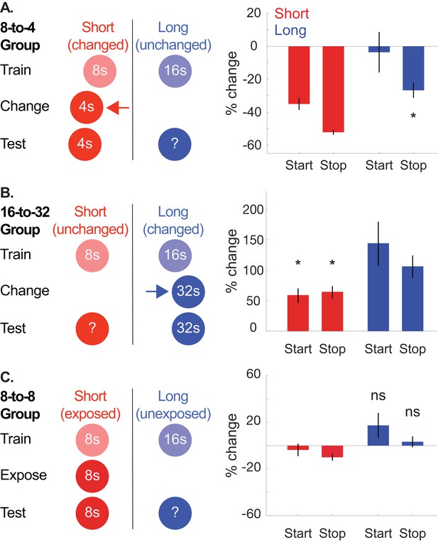
A and B depict design schematics (left panels) and average percent change in start/stop times (±SEM; right panels) for the 8-to-4 and 16-to-32 groups for Experiment 1, respectively.
(C) shows the same for the no-change control group.
-
Figure 1—figure supplement 2—source data 1
Data used to generate Figure 1—figure supplement 2.
- https://doi.org/10.7554/eLife.38790.006

Same as Figure 1—figure supplement 2, but showing single-trial averages (±SEM) for the remainder of the groups in the experiments (A, B, C, D, and E correspond to the 8-to-12 group of Experiment 2, both groups included in Experiment 3, the two Experiment 4 groups, and Experiment 5, respectively).
Three rats in Experiment 5 did not show any trials that met our criteria for being included in the single trial analysis (>2 responses and a start and stop time that occurred before and after the peak time, respectively). In those cases, they were omitted when computing the averages and statistics.
-
Figure 1—figure supplement 3—source data 1
Data used to generate Figure 1—figure supplement 3.
- https://doi.org/10.7554/eLife.38790.008
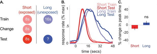
A depicts the design used for each phase in the no-change control group (n = 10).
(B) shows normalized response rate during training and testing. (C) shows percent change in peak times during testing (±SEM), relative to initial training.
-
Figure 2—source data 1
Data used to generate Figure 2.
- https://doi.org/10.7554/eLife.38790.012
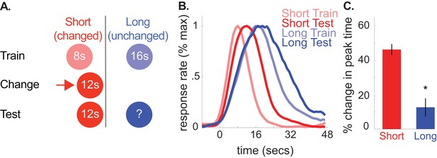
A shows the design used in the 8-to-12 group of the second experiment (n = 10).
(B) shows normalized responding during training and the test phases. (C) shows percent change in peak time for each cue during testing (±SEM), relative to initial training. Stars indicate significance.
-
Figure 3—source data 1
Data used to generate Figure 3.
- https://doi.org/10.7554/eLife.38790.014
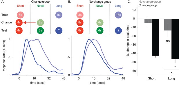
Top panels of A and B show designs used for the change (n = 5) and no-change (n = 5) groups of Experiment 3, respectively.
Mean normalized response rate for the critical, long cue during initial training and testing are plotted in the corresponding bottom panels. (C) shows percent change in peak times for the short and long cues in each group during testing (±SEM).
-
Figure 4—source data 1
Data used to generate Figure 4.
- https://doi.org/10.7554/eLife.38790.018
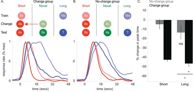
A and B show probe trial responding during initial training and testing for the short and long cues in the change (n = 5) and no-change (n = 5) groups of Experiment 3, respectively.
C shows percent change in peak time at test (±SEM) for both groups, relative to initial training.
-
Figure 4—figure supplement 1—source data 1
Data used to generate Figure 4—figure supplement 1.
- https://doi.org/10.7554/eLife.38790.017
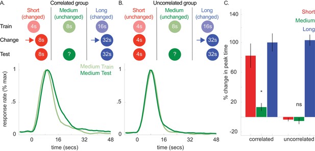
Top panels of A and B show designs used for the correlated (n = 5) and uncorrelated (n = 5) groups of Experiment 4a, respectively.
Mean normalized response rate for the critical, medium cue during initial training and testing are plotted in the corresponding bottom panels. (C) shows percent change in peak times for all cues in each group during testing (±SEM).
-
Figure 5—source data 1
Data used to generate Figure 5.
- https://doi.org/10.7554/eLife.38790.022
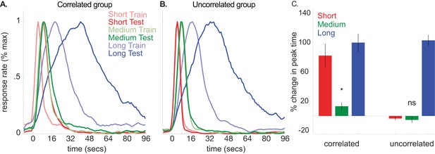
A and B show probe trial responding during initial training and testing for each cue in the correlated (n = 5) and uncorrelated (n = 5) groups of Experiment 4a, respectively.
(C) shows percent change in peak time at test (±SEM) for both groups and all cues, relative to initial training.
-
Figure 5—figure supplement 1—source data 1
Data used to generate Figure 5—figure supplement 1.
- https://doi.org/10.7554/eLife.38790.021
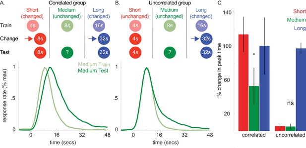
Top panels of (A) and (B) show designs used for the correlated (n = 5) and uncorrelated (n = 5) groups of Experiment 4b, respectively.
Mean normalized response rate for the critical, medium cue during initial training and testing are plotted in the corresponding bottom panels. (C) shows percent change in peak times for all cues in each group during testing (±SEM).
-
Figure 6—source data 1
Data used to generate Figure 6.
- https://doi.org/10.7554/eLife.38790.026
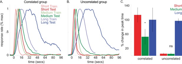
(A) and (B) show probe trial responding during initial training and testing for each cue in the correlated (n = 5) and uncorrelated (n = 5) groups of Experiment 4b, respectively.
(C) shows percent change in peak time at test (±SEM) for both groups and all cues, relative to initial training.
-
Figure 6—figure supplement 1—source data 1
Data used to generate Figure 6—figure supplement 1.
- https://doi.org/10.7554/eLife.38790.025
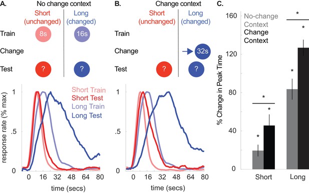
Top panels of (A) and (B) illustrate the design used in either context during Experiment 5 (n = 20).
Panels below each schematic show corresponding normalized response rates during training and during testing in either context. (C) shows percent change in peak time in either context during testing, relative to initial training (±SEM). Stars indicate significance.
-
Figure 7—source data 1
Data used to generate Figure 7.
- https://doi.org/10.7554/eLife.38790.028
Additional files
-
Source data 1
Compiled data and analyses for all experiments.
- https://doi.org/10.7554/eLife.38790.029
-
Transparent reporting form
- https://doi.org/10.7554/eLife.38790.030


