Polygenic adaptation on height is overestimated due to uncorrected stratification in genome-wide association studies
- Mashaal Sohail

- Robert M Maier
- Andrea Ganna
- Alex Bloemendal
- Alicia R Martin
- Michael C Turchin
- Joel Hirschhorn
- Mark J Daly
- Nick Patterson
- Benjamin Neale
- Iain Mathieson
- David Reich
- Shamil R Sunyaev
- Brigham and Women’s Hospital and Harvard Medical School, United States
- Harvard Medical School, United States
- Broad Institute of MIT and Harvard, United States
- Massachusetts General Hospital, United States
- Karolinska Institutet, Sweden
- University of Helsinki, Finland
- Brown University, United States
- University of Southern California, United States
- Boston Children’s Hospital, United States
- University of Pennsylvania, United States
- Howard Hughes Medical Institute, Harvard Medical School, United States
Figures
Figure 1 with 6 supplements

Polygenic height scores and tSDS scores based on GIANT and UK Biobank GWAS.
(a) Polygenic scores in present-day and ancient European populations are shown, centered by the average score across populations and standardized by the square root of the additive variance. Independent SNPs for the polygenic score from both GIANT (red) and the UK Biobank [UKB] (blue) were selected by picking the SNP with the lowest P value in each of 1700 independent LD blocks similarly to refs. (Berg et al., 2017; Racimo et al., 2018) (see Materials and methods). Present-day populations are shown from Northern Europe (CEU, GBR) and Southern Europe (IBS, TSI) from the 1000 genomes project; Ancient populations are shown in three meta-populations (HG = Hunter Gatherer (n = 162 individuals), EF = Early Farmer (n = 485 individuals), and SP = Steppe Ancestry (n = 465 individuals)) (see Supplementary file 2). Error bars are drawn at 95% credible intervals. See Figure 1—figure supplement 1 for analyses of concordance of effect size estimates between GIANT and UKB. See Figure 1—figure supplements 2–6 for polygenic height scores computed using other linkage disequilibrium pruning procedures, significance thresholds, summary statistics and populations. (b) tSDS for height-increasing allele in GIANT (left) and UK Biobank (right). The tSDS method was applied using pre-computed Singleton Density Scores for 4,451,435 autosomal SNPs obtained from 3195 individuals from the UK10K project (Field et al., 2016a; Field et al., 2016b) for SNPs associated with height in GIANT and the UK Biobank. SNPs were ordered by GWAS P value and grouped into bins of 1000 SNPs each. The mean tSDS score within each P value bin is shown on the y-axis. The Spearman correlation coefficient between the tSDS scores and GWAS P values, as well as the correlation standard errors and P values, were computed on the un-binned data. The gray line indicates the null-expectation, and the colored lines are the linear regression fit. The correlation is significant for GIANT (Spearman r = 0.078, p=1.55×10−65) but not for UK Biobank (Spearman r = −0.009, p=0.077). See Figure 1—source data 1 for figure data.
-
Figure 1—source data 1
Polygenic height scores and tSDS scores based on GIANT and UK Biobank GWAS.
- https://doi.org/10.7554/eLife.39702.009
Figure 1—figure supplement 1
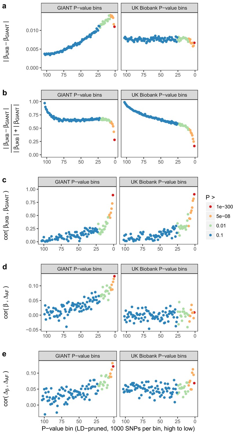
Beta concordance between GIANT and UK Biobank by P value bin.
SNPs intersecting between GIANT and UKB were LD-pruned (using PLINK 1.9 with parameters r^2 = 0.1, window size = 1 Mb, step size 5) and grouped into P value bins of 500 SNPs each, for P values from GIANT (left) and UKB (right). Color is based on the smallest P value in each bin. (a) Absolute beta difference. As expected, absolute beta and thus the absolute beta difference increases across P value bins. (b) Absolute beta difference, scaled by the sum of absolute betas. The relative difference of absolute betas decreases for lower P values. (c) Pearson correlation among betas approaches one for the lowest P values. (d) Correlation between beta (left GIANT, right UK Biobank) and GBR-TSI allele frequency difference. (e) Correlation between the GIANT - UK Biobank beta difference and GBR-TSI allele frequency difference.
Figure 1—figure supplement 2
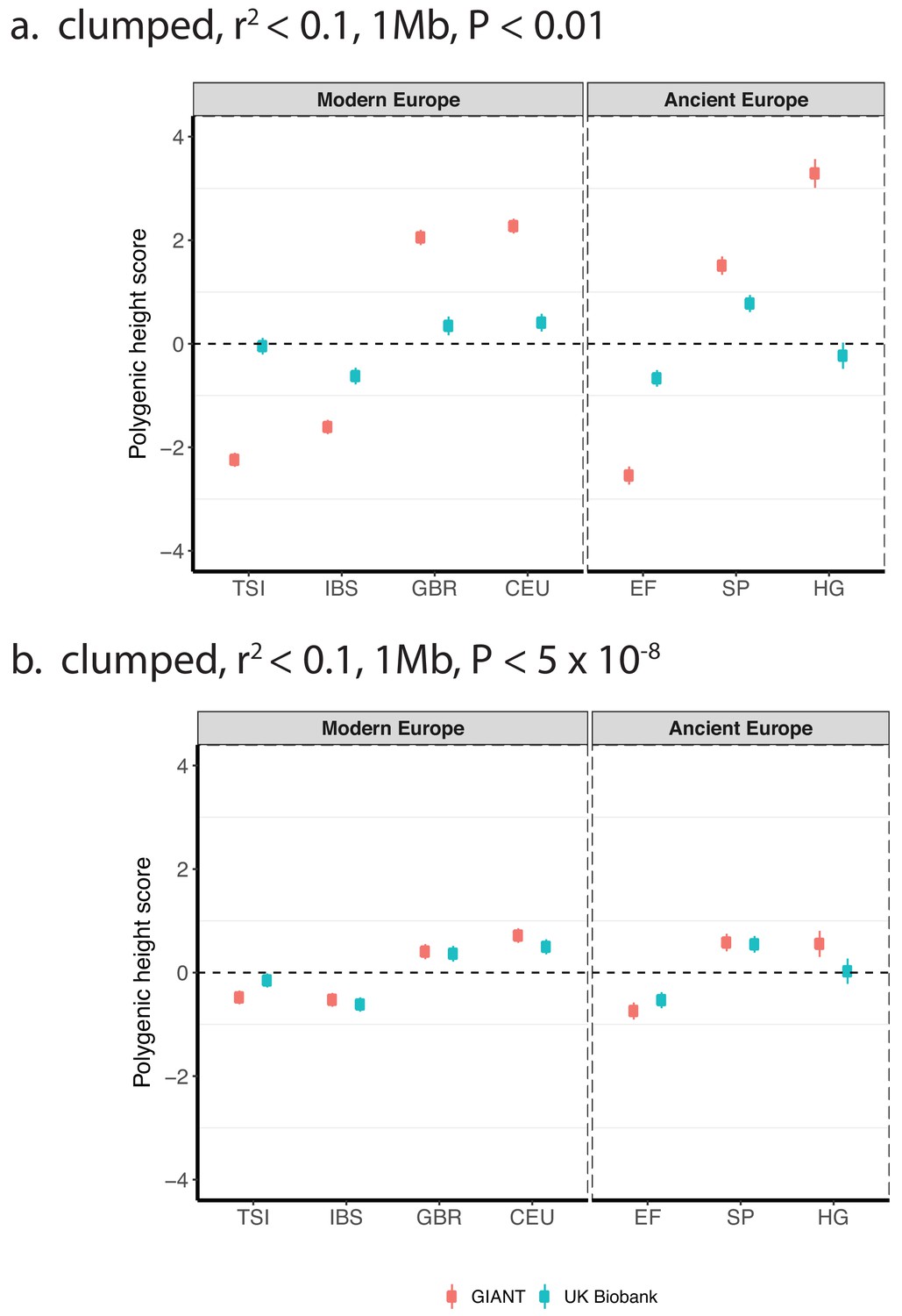
Polygenic height scores based on GIANT and UK Biobank GWAS for clumped SNPs in present-day and ancient Europeans.
Scores are shown, centered by the average score across modern and ancient populations respectively and standardized by the square root of the additive variance. SNPs were LD-pruned with plink’s clumping procedure for parameters: (a) r2 <0.1, 1 Mb, p<0.01 (81,941 SNPs in UKB, 22,561 SNPs in GIANT), and (b) r2 <0.1, 1 Mb, p<5×10⁻⁸ (4478 SNPs in UKB, 1442 SNPs in GIANT). Modern populations are shown from Northern Europe (CEU, GBR) and Southern Europe (IBS, TSI) from the 1000 genomes project. Ancient populations are shown in three meta-populations (HG = Hunter Gatherer (n = 162 individuals), EF = Early Farmer (n = 485 individuals), and SP = Steppe Ancestry (n = 465 individuals)). Error bars are drawn at 95% credible intervals.
Figure 1—figure supplement 3
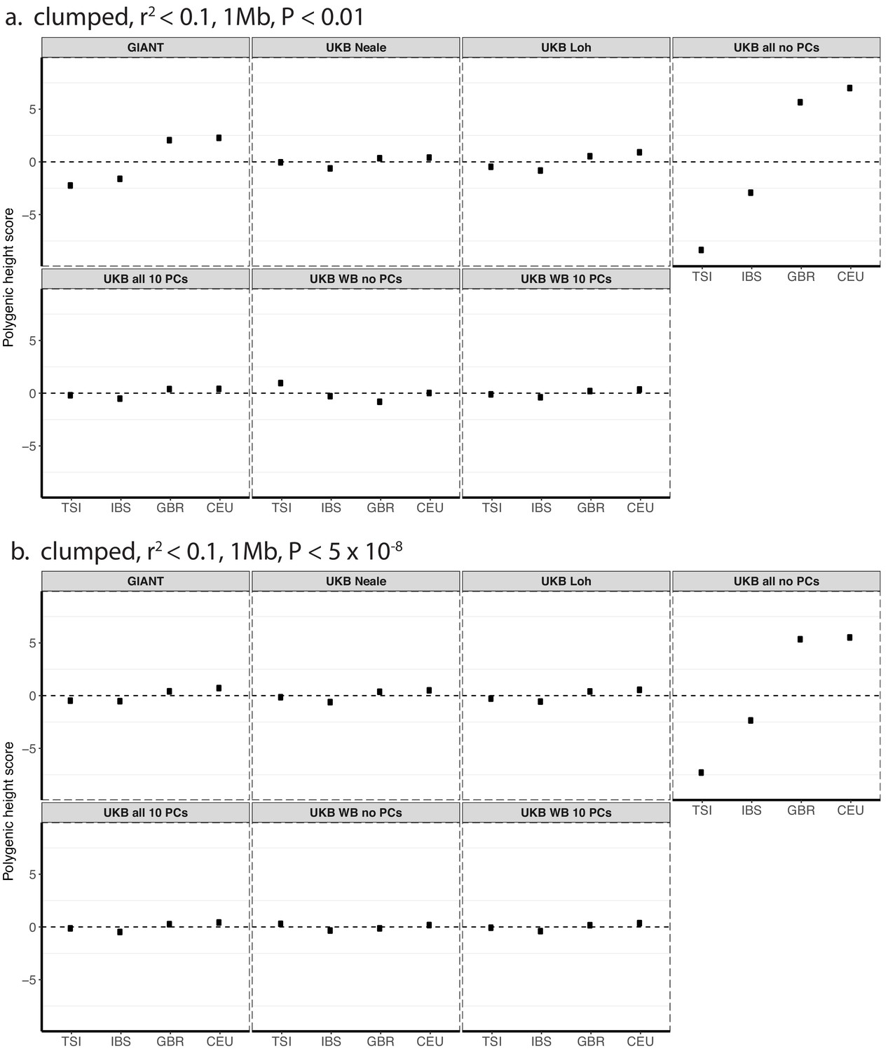
Polygenic height scores in 1000 genomes European populations using clumped SNPs and effect sizes from different summary statistics.
Polygenic scores in modern European populations are shown using SNPs LD-pruned with PLINK’s clumping procedure with parameters: (a) r2 <0.1, 1 Mb, p<0.01, and (b) r2 <0.1, 1 Mb, p<5×10⁻⁸. Scores are centered by the average score across populations and standardized by the square root of the additive variance. Modern populations are shown from Northern Europe (CEU, GBR) and Southern Europe (IBS, TSI) from the 1000 Genomes Project. Error bars are drawn at 95% credible intervals.
Figure 1—figure supplement 4
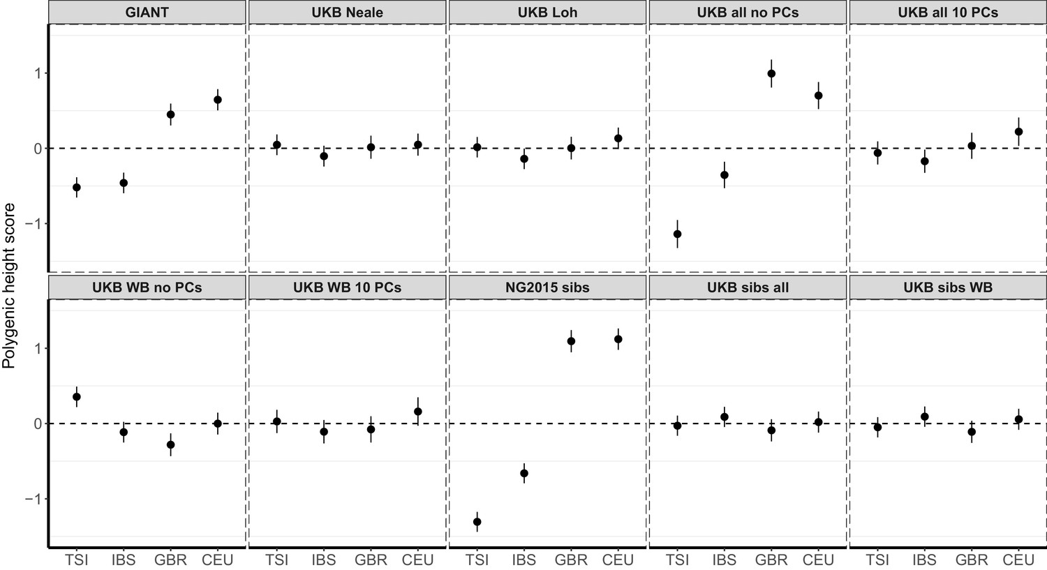
Polygenic height scores in 1000 Genomes Project European populations using ~1700 independent SNPs and effect sizes from different summary statistics.
Polygenic scores in modern European populations are shown using SNPs LD-pruned by picking the SNP with the lowest P value in each of ~1700 LD-independent blocks genome-wide. Scores are centered by the average score across populations and standardized by the square root of the additive variance. Modern populations are shown from Northern Europe (CEU, GBR) and Southern Europe (IBS, TSI) from the 1000 Genomes Project. Error bars are drawn at 95% credible intervals.
Figure 1—figure supplement 5
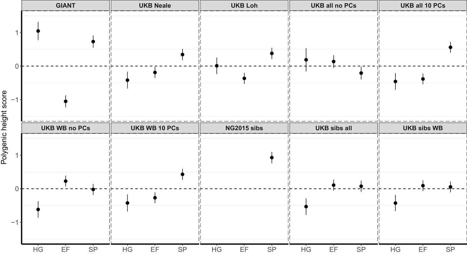
Polygenic height scores in ancient populations using ~1700 independent SNPs and effect sizes from different summary statistics.
Polygenic scores in ancient meta-populations are shown using SNPs LD-pruned by picking the SNP with the lowest P value in each of ~1700 LD-independent blocks genome-wide. Scores are centered by the average score across populations and standardized by the square root of the additive variance. Error bars are drawn at 95% credible intervals. Ancient populations are shown in three meta-populations (HG = Hunter Gatherer (n = 162 individuals), EF = Early Farmer (n = 485 individuals), and SP = Steppe Ancestry (n = 465 individuals)). The y-axis is truncated at (−1.5, 1.5) for all panels – this omits two points in the NG2015 sibs panel: HG [3.86 (CI: 3.60, 4.12)], EF [−2.18(CI: −2.34,–2.02)].
Figure 1—figure supplement 6

Polygenic height scores in ancient and global modern populations using three different GWAS.
All scores are centered by the average score across all populations () and standardized by the square root of the additive variance. Error bars are drawn at 95% credible intervals. Modern populations are shown from Northern Europe (CEU, GBR), Southern Europe (IBS, TSI), South Asia (PJL, BEB), East Asia (CHB, JPT) and Africa (YRI, LWK). Ancient populations are shown in three meta-populations (HG = Hunter-Gatherer (n=162 individuals), EF = Early Farmer (n=485 individuals), and SP = Steppe Ancestry (n=465 individuals)). Pseudo-haploid genotype calls were made for modern populations before computing polygenic scores to allow fair comparison with ancient DNA. SNPs were LD-pruned by picking the SNP with the lowest P value in each of ~1700 LD-independent blocks genome-wide.
Figure 2 with 4 supplements
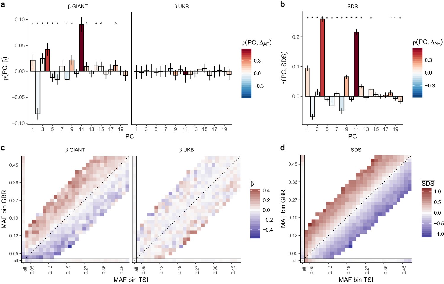
Evidence of stratification in height summary statistics.
Top row: Pearson Correlation coefficients of (a) PC loadings and height beta coefficients from GIANT and UKB, and (b) PC loadings and SDS (pre-computed in the UK10K) across all SNPs. PCs were computed in all 1000 genomes phase one samples (Abecasis et al., 2012). Colors indicate the correlation of each PC loading with the allele frequency difference between GBR and TSI, a proxy for the European North-South genetic differentiation. PC 4 and 11 are most highly correlated with the GBR - TSI allele frequency difference. Confidence intervals and P values are based on Jackknife standard errors (1000 blocks). Open circles indicate correlations significant at alpha = 0.05, stars indicate correlations significant after Bonferroni correction in 20 PCs (p<0.0025). Bottom row: Heat map after binning all SNPs by GBR and TSI minor allele frequency of (c) mean beta coefficients from GIANT and UKB, and (d) SDS scores for all SNPs. Only bins with at least 300 SNPs are shown. While the stratification effect in SDS is not unexpected, it can lead to false conclusions when applied to summary statistics that exhibit similar stratification effects. See Figure 2—figure supplements 1–3 for analyses of stratification effects in different summary statistics, and Supplementary file 3 for further description of stratification effects. UKB height betas exhibit stratification effects that are weaker, and in the opposite direction of the stratification effects in GIANT (see Figure 2—figure supplement 4 for a possible explanation). See Figure 2—source data 1 for figure data.
-
Figure 2—source data 1
Evidence of stratification in height summary statistics.
- https://doi.org/10.7554/eLife.39702.015
Figure 2—figure supplement 1
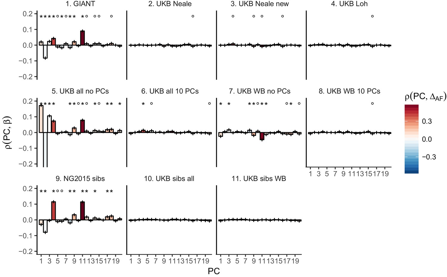
Pearson Correlation coefficients of PC loadings and height beta coefficients for different summary statistics.
PCs were computed in all 1000 genomes phase one samples. Colors indicate the correlation of each PC loading with the allele frequency difference between GBR and TSI, a proxy for the European North-South genetic differentiation. PC 4 and 11 are most highly correlated with the GBR - TSI allele frequency difference. Error bars indicate 95% confidence interval of the correlation coefficient, assuming 60,000 independent genetic markers. We confirmed that the resulting standard error estimates are similar to block jackknife standard error estimates. Open circles indicate correlations significant at alpha = 0.05, stars indicate correlations significant after Bonferroni correction in 20 PCs (p<0.0025).
Figure 2—figure supplement 2
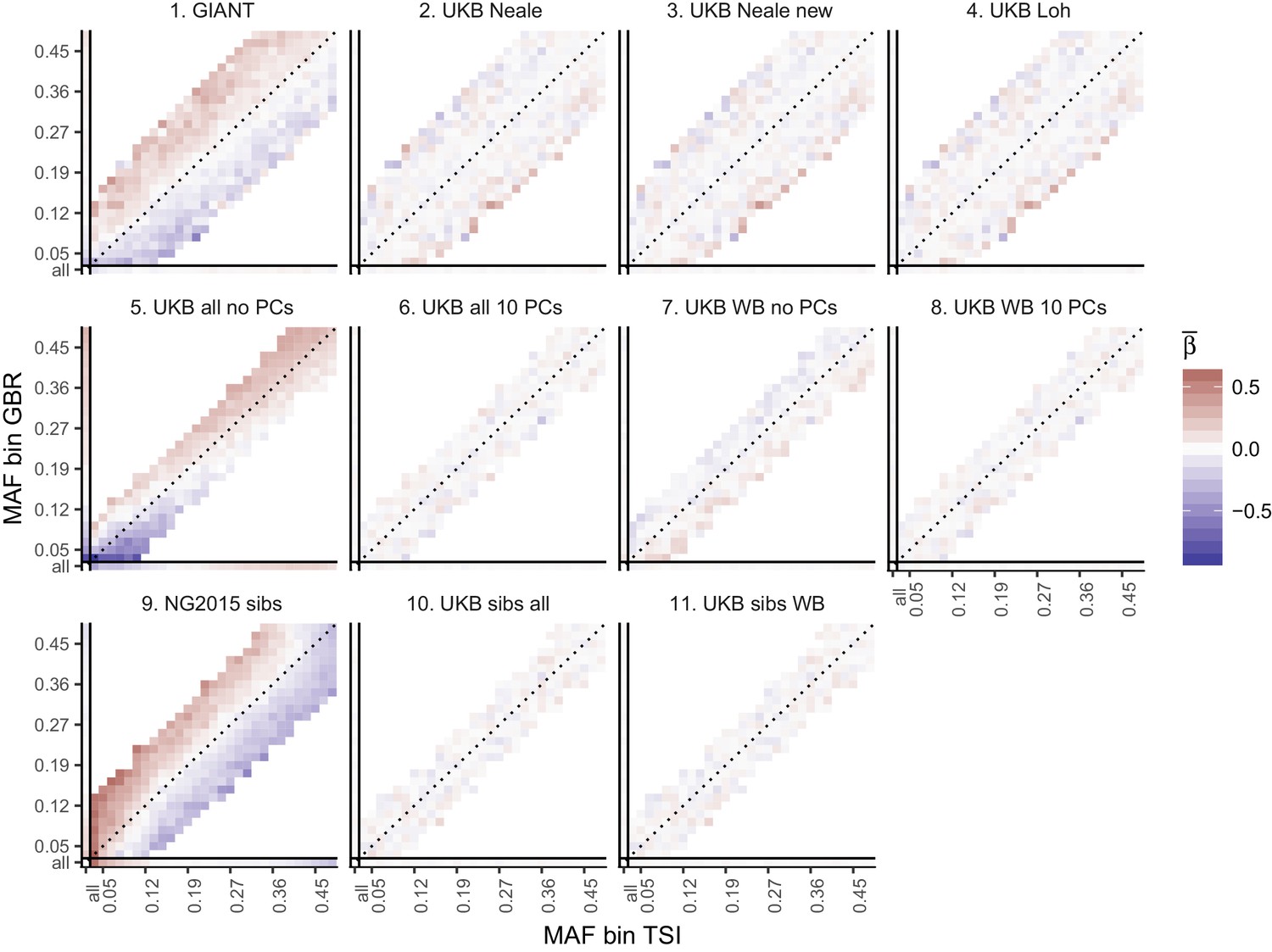
Heat map of mean beta coefficients for different summary statistics.
All SNPs are binned by GBR and TSI minor allele frequency. Only bins with at least 300 SNPs are shown. Panel 7 (as well as 2, 3 and 4) shows stratification effects in opposite direction to those in GIANT. Figure 2—figure supplement 4 illustrates how these opposite-direction stratification effects can arise.
Figure 2—figure supplement 3

Effect of GBR-TSI allele frequency difference on beta estimates and P values.
SNPs with MAF >0.2 (based on mean between TSI and GBR) were grouped into GBR-TSI allele frequency difference deciles, with the first decile representing SNPs less common in GBR and the last decile representing SNPs more common in GBR. (a) Fraction of height-increasing (yellow dots) vs. height-decreasing SNPs (purple dots) in each decile. In GIANT, 59% of SNPs in the highest decile are estimated to be height-increasing, and 41% are estimated to be height-decreasing. In the UK Biobank, this ratio is close to 50–50. (b) Lambda-GC in each decile for height-increasing (yellow dots) vs. height-decreasing SNPs (purple dots). In GIANT, the median P value of SNPs in the highest decile is 2.78 for SNPs estimated to be height-increasing and 1.83 for SNPs estimated to be height-decreasing (a difference of 52%). In the UK Biobank, the median P value of SNPs in the highest decile is 2.65 for SNPs estimated to be height-increasing and 2.89 for SNPs estimated to be height-decreasing (a difference of only 9%, going in the opposite direction).
Figure 2—figure supplement 4
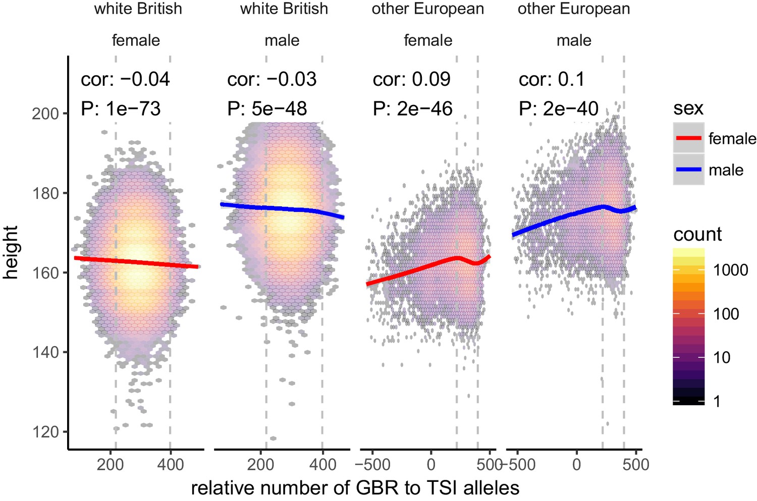
Height (cm) in the UKB as a function of GBR-TSI score.
We computed the relative number of GBR to TSI related alleles in each sample by multiplying the allele frequency difference by the number of alternative alleles in each sample in the UKB (GBR-TSI score). Vertical lines indicate 5th and 95th percentile of among-white British samples, showing that there is a significant negative relationship between the GBR-TSI allele sharing score and height (in cm). Among all other broadly European samples, this relationship is significantly positive across the whole range, but again significantly negative in the white British range. This can explain why stratification effects go in opposite directions in a UKB height GWAS of white British samples and a UKB height GWAS of all samples. Here, other European samples were defined as those that lie within the mean ±24 standard deviations along the first six principal components.
Figure 3 with 5 supplements
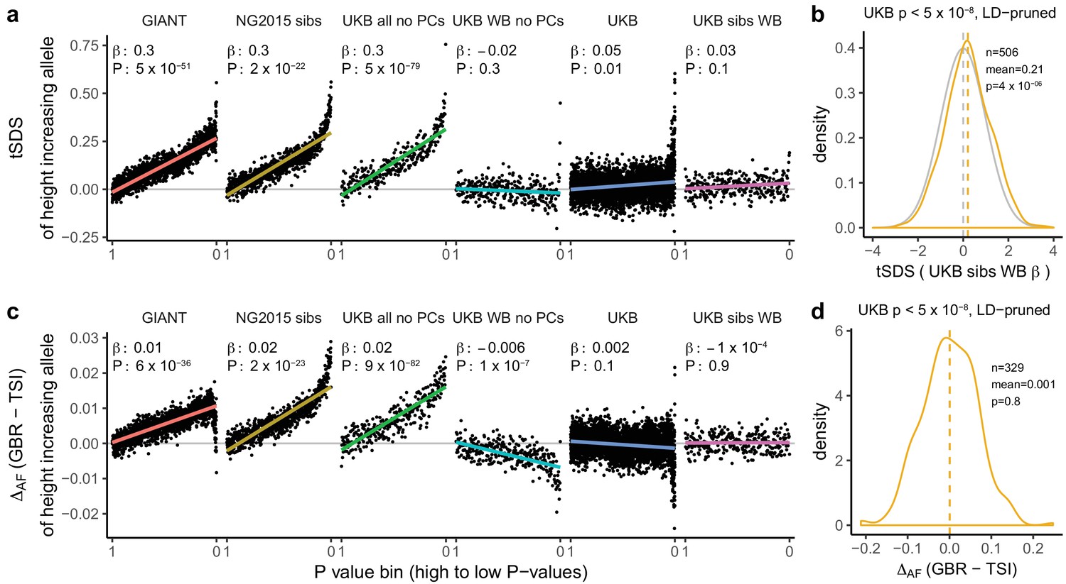
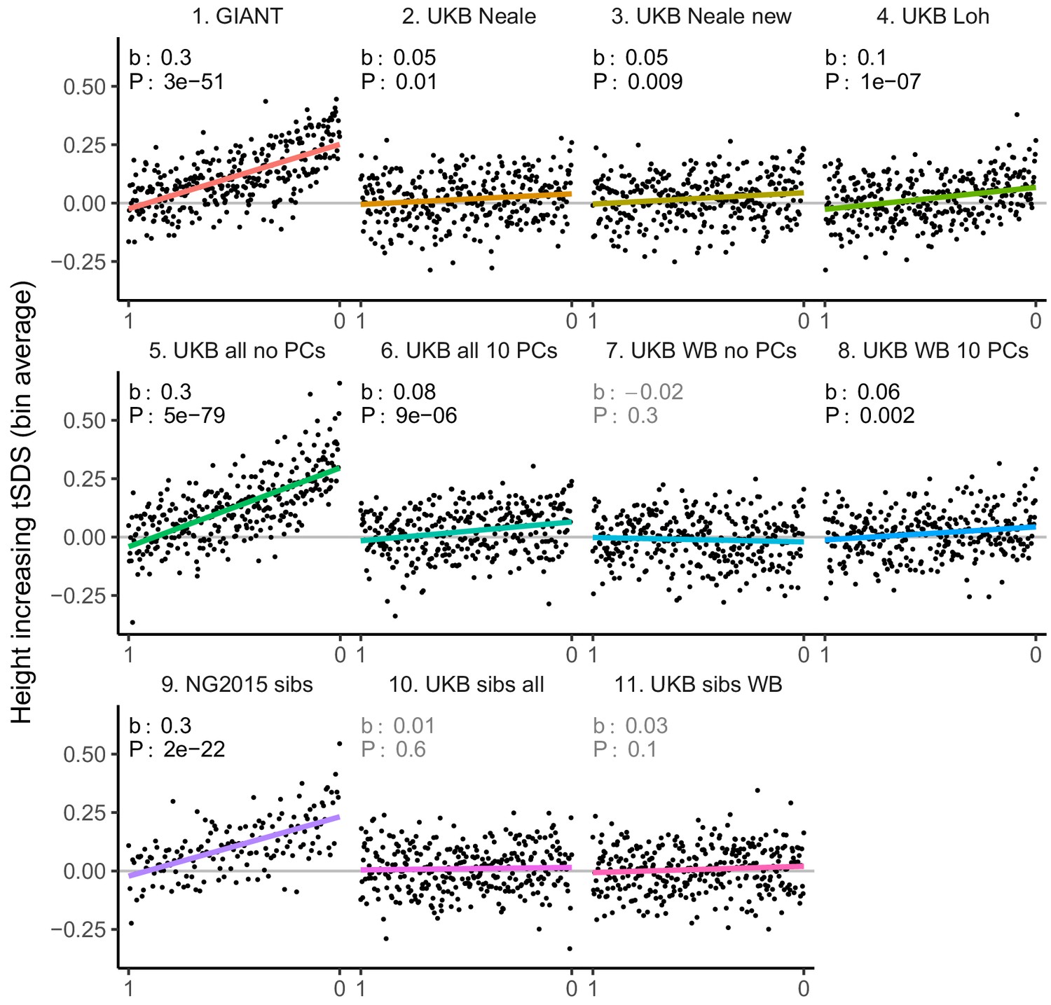
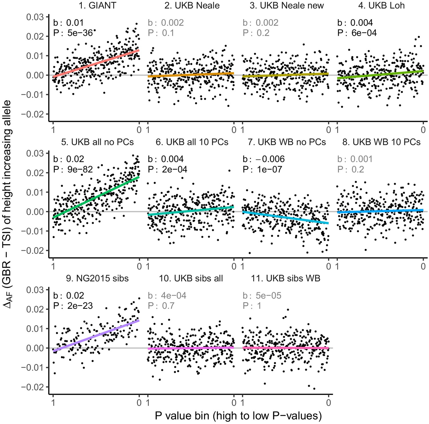
Height tSDS results for different summary statistics.
(a) Mean tSDS of the height increasing allele in each P value bin for six different summary statistics. The first two panels are computed analogously to Figure 4A and Figure S22 of Field et al. (2016a). In contrast to those Figures and to Figure 1b, the displayed betas and P values correspond to the slope and P value of the linear regression across all un-binned SNPs (rather than the Spearman correlation coefficient and Jackknife P values). The y-axis has been truncated at 0.75, and does not show the top bin for UKB all no PCs, which has a mean tSDS of 1.5. (b) tSDS distribution of the height increasing allele in 506 LD-independent SNPs which are genome-wide significant in a UKB height GWAS, where the beta coefficient is taken from a within sibling analysis in the UKB. The gray curve represents the standard normal null distribution, and we observe a significant shift. (c) Allele frequency difference between GBR and TSI of the height increasing allele in each P value bin for six different summary statistics. Betas and P values correspond to the slope and P value of the linear regression across all un-binned SNPs. The lowest P value bin in UKB all no PCs with a y-axis value of 0.06 has been omitted. (d) Allele frequency difference between GBR and TSI of the height increasing allele in 329 LD-independent SNPs which are genome-wide significant in a UKB height GWAS and were intersected with our set of 1000 genomes SNPs. There is no significant difference in frequency in these two populations, suggesting that tSDS shift at the genome-wide significant SNPs is not driven by population stratification at least due to this particular axis. The patterns shown here suggest that the positive tSDS values across the whole range of P values is a consequence of residual stratification. At the same time, the increase in tSDS at genome-wide significant, LD-independent SNPs in (b) cannot be explained by GBR - TSI allele frequency differences as shown in (d). See Figure 3—figure supplements 1–4 for other GWAS summary statistics for unpruned and LD-pruned SNPs. Binning SNPs by P value without LD-pruning can lead to unpredictable patterns at the low P value end, as the SNPs at the low P value end are less independent of each other than higher P value SNPs (Figure 3—figure supplement 5). See Figure 3—source data 1 for figure data.
-
Figure 3—source data 1
Height tSDS results for different summary statistics.
- https://doi.org/10.7554/eLife.39702.022
Figure 3—figure supplement 1
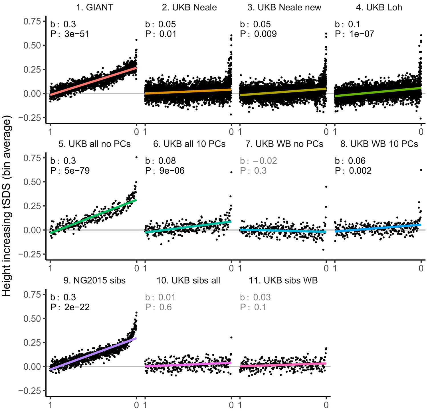
tSDS for height-increasing alleles using effect sizes from different summary statistics.
SNPs were ordered by GWAS P value and grouped into bins of 1000 SNPs each. The mean tSDS score within each P value bin is shown on the y-axis. In contrast to Figure 3, where Spearman correlation coefficients and Jackknife standard errors were computed, here we show the regression slope and P value, which were computed on the un-binned data. The gray line indicates the null-expectation, and the colored lines are the linear regression fit. The lowest P value bin in panel five with a y-axis value of 1.5 has been omitted.
Figure 3—figure supplement 2
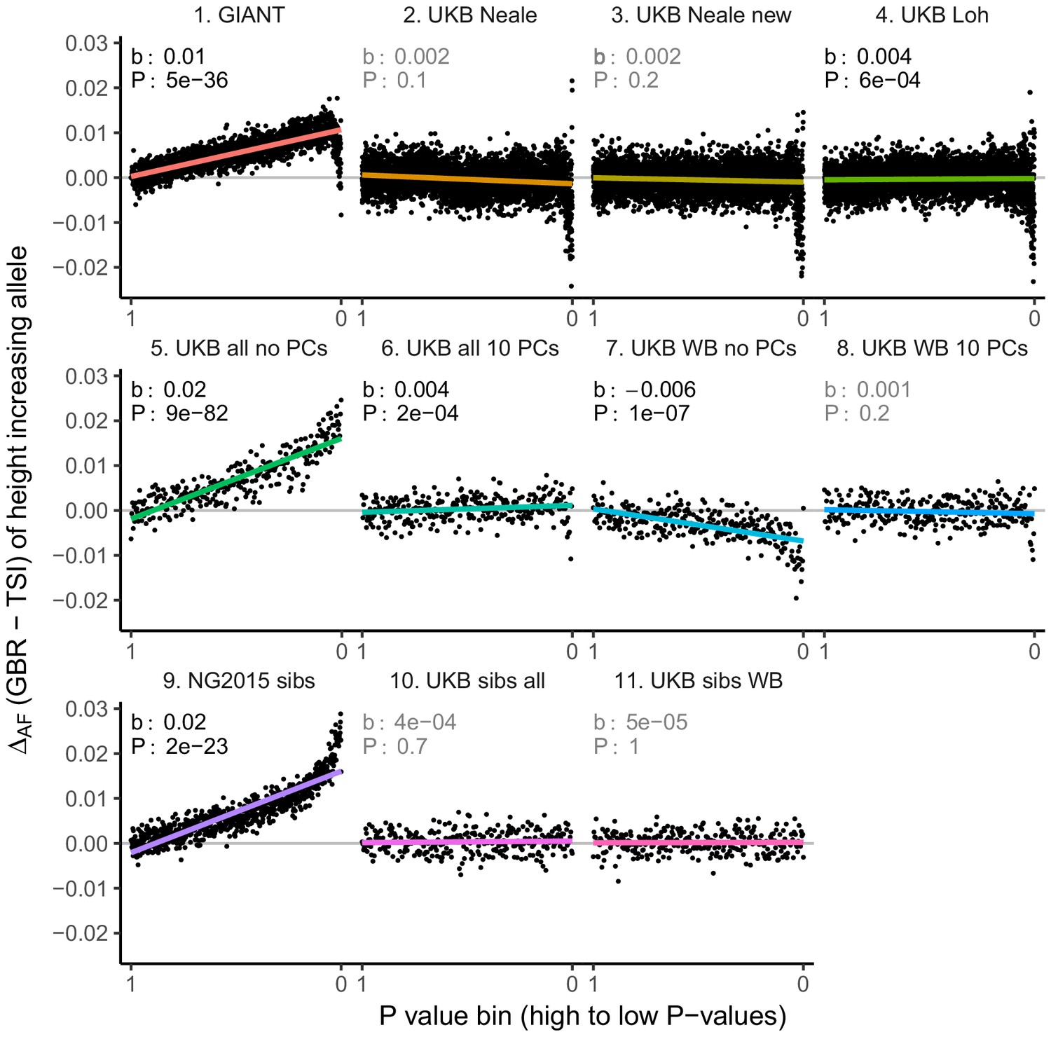
Allele frequency difference for height-increasing alleles using different summary statistics.
SNPs were ordered by GWAS P value and grouped into bins of 1000 SNPs each. The gray line indicates the null-expectation, and the colored lines are the linear regression fit. The lowest P value bin in panel five with a y-axis value of 0.06 has been omitted.
Figure 3—figure supplement 3
tSDS for LD-pruned height-increasing alleles using effect sizes from different summary statistics.
Binning SNPs by P value can lead to spurious results at the low P value bins when SNPs are in LD (Figure 3—figure supplement 5). Here, LD-pruned SNPs were ordered by GWAS P value and grouped into bins of 100 SNPs each. The mean tSDS score within each P value bin is shown on the y-axis. In contrast to Figure 3, where Spearman correlation coefficients and Jackknife standard errors were computed, here we show the regression slope and P value, which were computed on the un-binned data. The gray line indicates the null-expectation, and the colored lines are the linear regression fit.
Figure 3—figure supplement 4
Allele frequency difference for LD-pruned height-increasing alleles using different summary statistics.
Binning SNPs by P value can lead to spurious results at the low P value bins when SNPs are in LD (Figure 3—figure supplement 5). Here, LD-pruned SNPs were ordered by GWAS P value and grouped into bins of 100 SNPs each. The gray line indicates the null-expectation, and the colored lines are the linear regression fit.
Figure 3—figure supplement 5

Number of independent regions per GWAS P value bin in the UK Biobank.
SDS results in Field et al. as well as in Figure 3 in this article are visualized by grouping non-independent SNPs into bins according to their P value. This may lead to unpredictable patterns at the low end of the P value distribution, because the lowest P value bins do not represent independent signals. This is demonstrated here, by grouping all UKB SNPs into bins of 1000 SNPs each, as in the SDS plots in Figure 1b and Figure 3. Left: The number of independent SNPs per P value bin is much lower at lower P values. Right: Neighboring P value bins share a large fraction of 1 Mb regions at lower P values. This demonstrates that the lowest P value bins do not represent independent signals if SNPs are not LD-pruned and can exhibit patterns that are dominated by one or a few LD-regions.
Figure 4 with 4 supplements
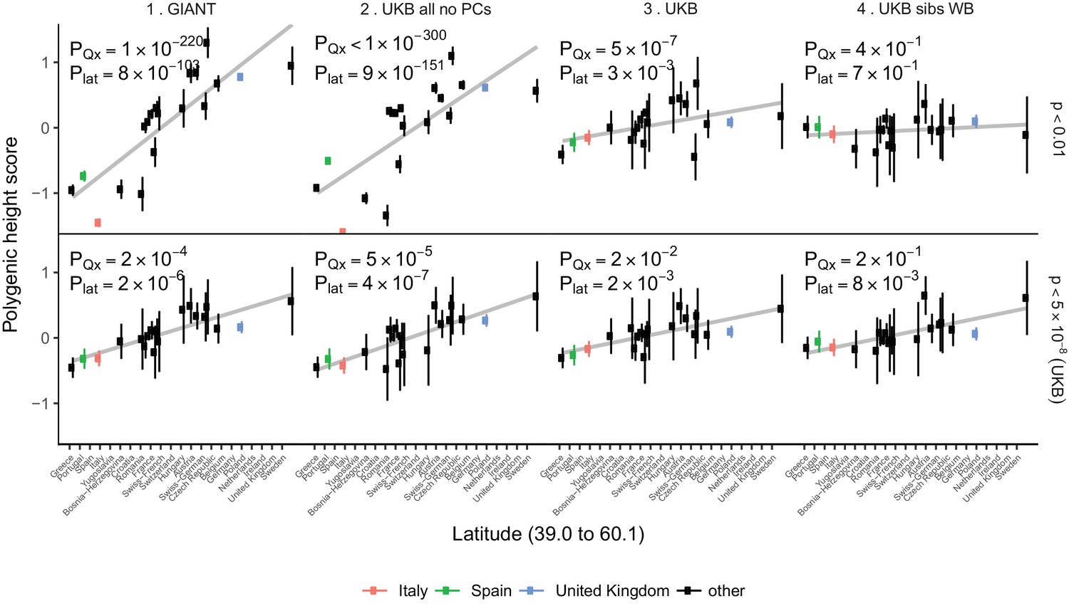
Polygenic height scores in POPRES populations show a residual albeit attenuated signal of polygenic adaptation for height.
Standardized polygenic height scores from four summary statistics for 19 POPRES populations with at least 10 samples per population, ordered by latitude (see Supplementary file 4). The grey line is the linear regression fit to the mean polygenic scores per population. Error bars represent 95% confidence intervals and are calculated in the same way as in Figure 1. SNPs which were overlapping between each set of the summary statistics and the POPRES SNPs were clumped using PLINK 1.9 with parameters r^2 < 0.1, 1 Mb distance, p<1. (Top) A number of independent SNPs was chosen for each summary statistic to match the number of SNPs which remained when clumping UKB at p<0.01. (Bottom) A set of independent SNPs with p<5×10⁻⁸ in the UK Biobank was selected and used to compute polygenic scores along with effect size estimates from each of the different summary statistics. The numbers on each plot show the Qx P value and the latitude covariance P value respectively for each summary statistic. See Figure 4—figure supplements 1–4 for other clumping strategies and GWAS summary statistics. See Figure 4—source data 1 for figure data.
-
Figure 4—source data 1
Polygenic height scores in POPRES populations show a residual albeit attenuated signal of polygenic adaptation for height.
This reference was updated from its bioRxiv version to its now published version.
- https://doi.org/10.7554/eLife.39702.028
Figure 4—figure supplement 1

Polygenic height scores in POPRES for different summary statistics.
Standardized polygenic height score from diverse summary statistics for 19 POPRES populations with at least 10 samples per population, ordered by latitude (see Supplementary file 4). Confidence intervals and clumping procedure are the same as in (a). The gray line is the linear regression fit to the mean polygenic height score per population. The numbers on each plot show the Qx P value, the latitude covariance P value and the number of SNPs respectively for each summary statistic. Each column shows a different selection of SNPs. clump all: clumped SNPs with no P value threshold; clump 0.01: clumped SNPs with p<0.01 in UKB and the same number of SNPs in other summary statistics (same as Figure 4); clumpwindow 1.5M: genome was split into blocks of 1.5 Mb, lowest P-value SNP was picked in each bin, similar to the 1700 blocks; ldwindow 1.5 Mb: genome was split into blocks of 1.5 Mb, random SNP was picked in each bin; UKB sig: LD-pruned SNPs with p<5×10⁻⁸ in UKB.
Figure 4—figure supplement 2
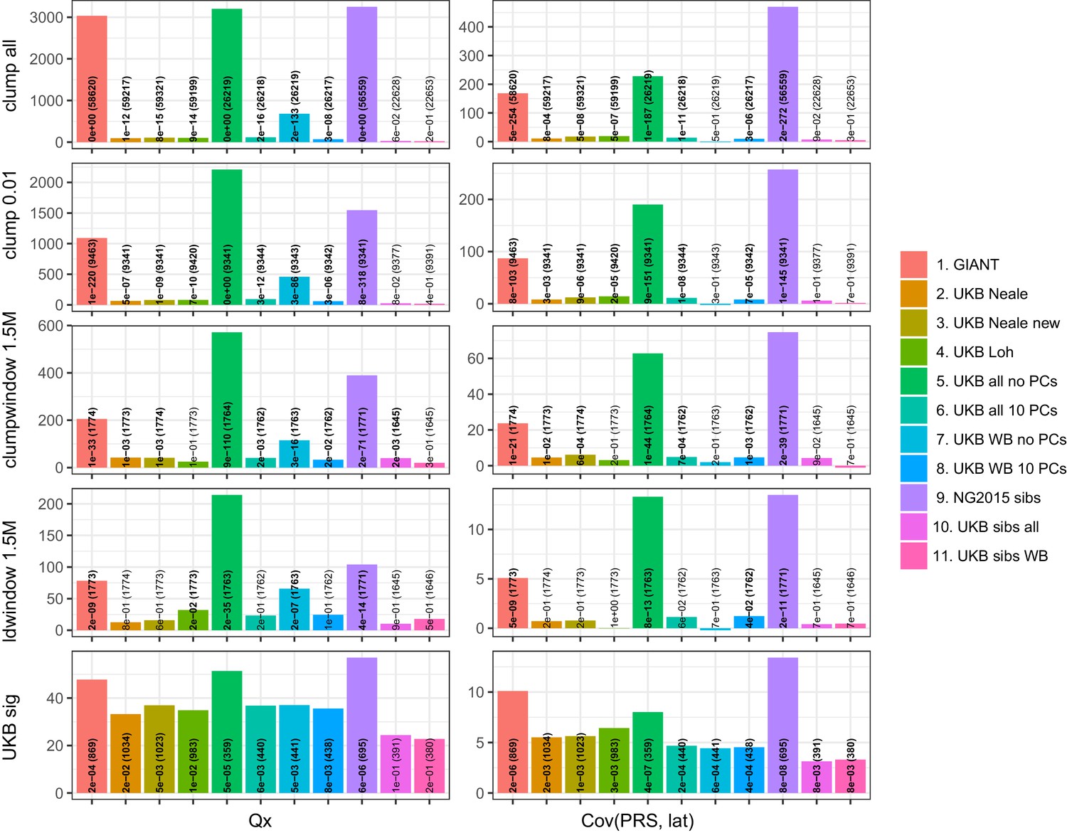
Test statistics for Qx (left) and latitude correlation (right) in the POPRES dataset for different summary statistics.
The numbers indicate P values and the number of SNPs, and numbers in bold highlight nominal significance (p<0.05).
Figure 4—figure supplement 3
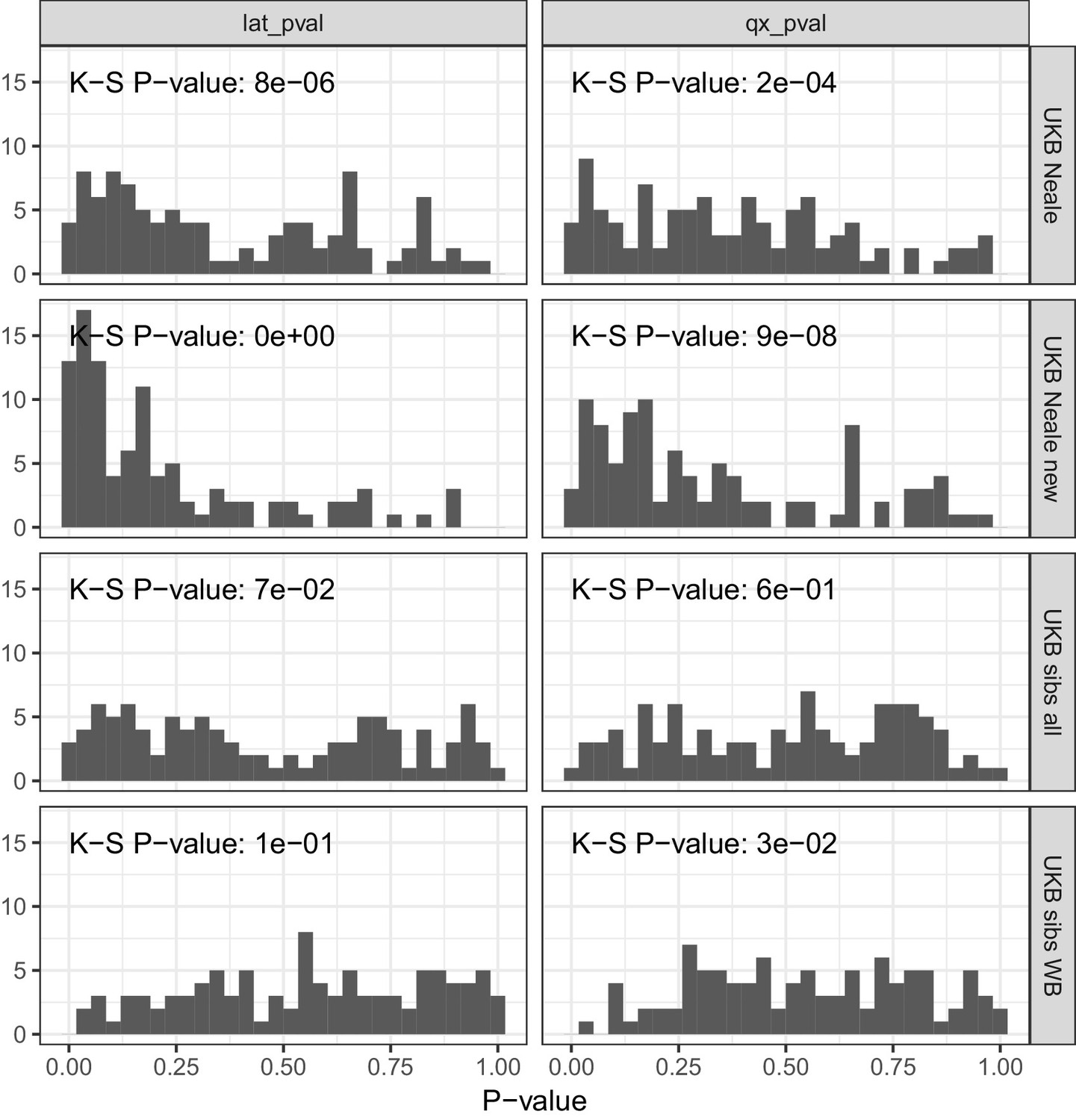
P value calibration in the POPRES dataset for Qx and latitude covariance tests.
Random sets of around 1700 independent markers were drawn in 100 repetitions for four summary statistics and Qx and latitude P values were computed. In UK Biobank sibling estimates this resulted in a uniform P value distribution (non-significant Kolmogorov–Smirnov test), while an inflation was observed for UK Biobank GWAS summary statistics.
Figure 4—figure supplement 4

Spearman correlations between polygenic height scores in the POPRES dataset computed from different summary statistics.
Spearman correlation coefficients of mean population polygenic score ranking for all pairs of summary statistics at different SNP selections. Polygenic scores from independent SNPs which are genome-wide significant in UKB lead to more consistent rankings than PRS from other sets of SNPs, despite having lower prediction power. Each column shows a different selection of SNPs. clump all: clumped SNPs with no P value threshold; clump 0.01: clumped SNPs with p<0.01 in UKB and the same number of SNPs in other summary statistics (same as Figure 4); clumpwindow 1.5M: genome was split into blocks of 1.5 Mb, lowest P-value SNP was picked in each bin, similar to the 1700 blocks; ldwindow 1.5 Mb: genome was split into blocks of 1.5 Mb, random SNP was picked in each bin; UKB sig: LD-pruned SNPs with p<5×10⁻⁸in UKB.
Author response image 1

Additional files
-
Supplementary file 1
Description of 11 GWAS summary statistics.
- https://doi.org/10.7554/eLife.39702.029
-
Supplementary file 2
Table of ancient and 1000 genomes modern populations used with sample sizes.
- https://doi.org/10.7554/eLife.39702.030
-
Supplementary file 3
Supplementary note on characterization of stratification effects in GIANT and UK Biobank.
- https://doi.org/10.7554/eLife.39702.031
-
Supplementary file 4
Table of POPRES populations used with sample sizes and latitude.
- https://doi.org/10.7554/eLife.39702.032
-
Supplementary file 5
LD Score regression estimates for 11 different summary statistics.
LD score regression can be used to detect residual stratification effects in summary statistics, and so we tested whether LDSC confirms our hypothesis of residual stratification. We detect a greatly inflated intercept estimate of 9.42 in UKB all no PCs, but only a moderately increased intercept value in GIANT and an intercept less than one in NG2015 sibs. The relatively small GIANT intercept can be explained by cohort-wise lambda-GC correction, while the low intercept in NG2015 sibs is possibly caused by the adaptive permutation procedure which does not compute precise p-values for non-significant associations. In both cases LDSC cannot be expected to pick up stratification effects, since the generation of summary statistics is not in line with the LDSC model.
- https://doi.org/10.7554/eLife.39702.033
-
Supplementary file 6
Correlation of beta estimates at all 86,153 shared SNPs.
- https://doi.org/10.7554/eLife.39702.034
-
Supplementary file 7
Correlation of beta estimates at 2251 shared SNPs which are significant in the UK Biobank.
- https://doi.org/10.7554/eLife.39702.035
-
Transparent reporting form
- https://doi.org/10.7554/eLife.39702.036
Download links
A two-part list of links to download the article, or parts of the article, in various formats.
Downloads (link to download the article as PDF)
Open citations (links to open the citations from this article in various online reference manager services)
Cite this article (links to download the citations from this article in formats compatible with various reference manager tools)
Polygenic adaptation on height is overestimated due to uncorrected stratification in genome-wide association studies
eLife 8:e39702.
https://doi.org/10.7554/eLife.39702


