Figures and data in Mechanics and dynamics of translocating MreB filaments on curved membranes | eLife

Figures
Additional files

6 figures and 3 additional files

Figures

Figure 1 with 1 supplement

Download asset Open asset

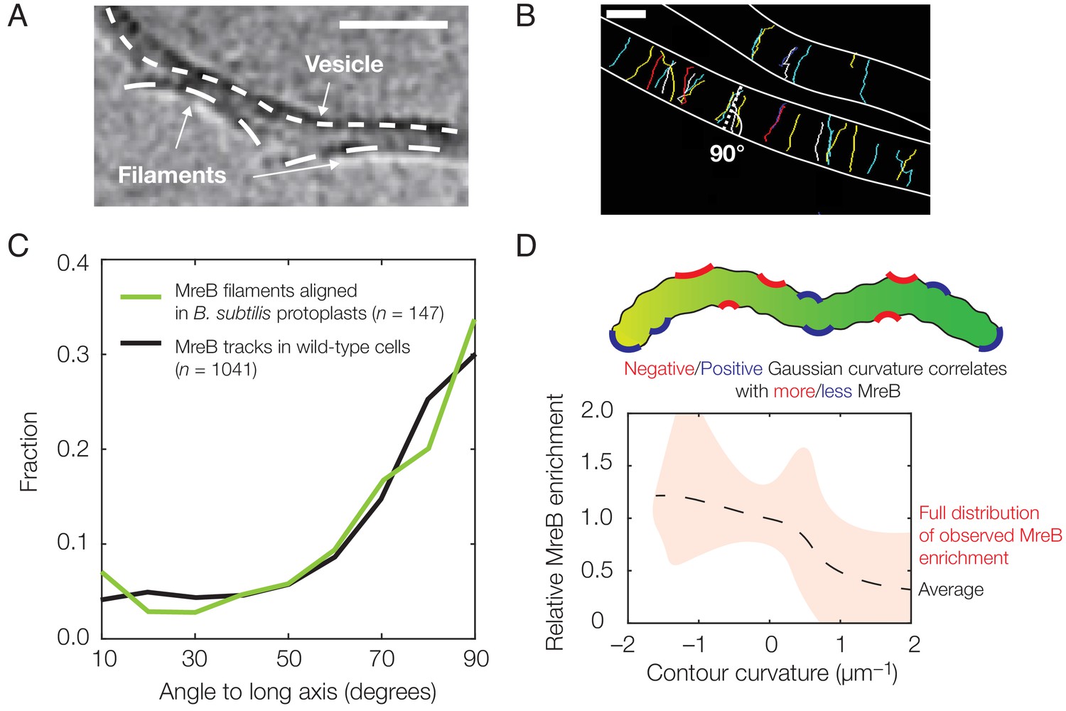
Experimental observation of membrane binding and translocation.

(A) Cryo-electron microscopy image showing the direct membrane binding of MreB filaments reconstituted in vitro to vesicles. The scale bar indicates 50 nm, and dashed curves represent guides. The image is reproduced here from Salje et al. (2011) under a CC BY 3.0 license (https://creativecommons.org/licenses/by/3.0/). (B) Fluorescence microscopy image of MreB filaments translocating in live Bacillus subtilis cells with trajectories of individual filaments drawn and cell edges outlined, reproduced from Hussain et al. (2018) (see also Figure 1—video 1). Note that typical trajectories are perpendicular to the cellular long axis, consistent with the binding angles in (C). The scale bar indicates 1 μm. (C) Angular distribution of membrane-bound filaments within B. subtilis protoplasts confined to become rod-shaped (green curve) and MreB motion in wild-type B. subtilis cells (black curve), reproduced from Hussain et al. (2018). (D) Relative MreB enrichment in Escherichia coli cells growing in a sinusoidally shaped chamber, adapted from Ursell et al. (2014).

https://doi.org/10.7554/eLife.40472.002

Figure 1—video 1

Download asset

posterframe for video — SIM-TIRF movies of MreB motion.

(Left) E. coli containing msfGFP-MreB(sw) (strain NO50 from Ouzounov et al., 2016) grown in M9 glucose at 37°C. The time between frames is 2 s. (Right) B. subtilis containing MreB-mNeonGreen (strain YS09 from Hussain et al., 2018) grown in CH media at 37°C. The time between frames is 1 s.

https://doi.org/10.7554/eLife.40472.003

Figure 2 with 1 supplement

Download asset Open asset

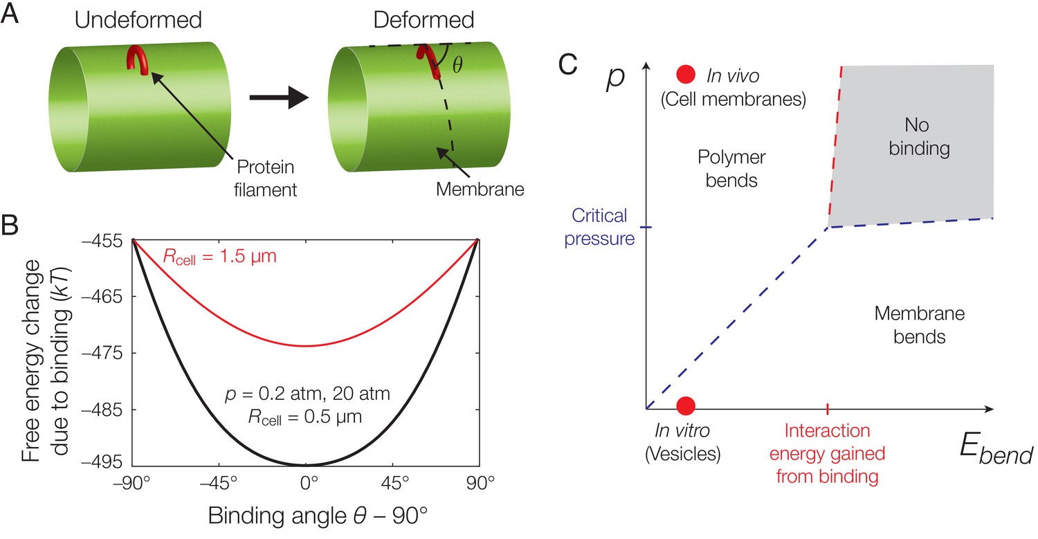
Mechanics of binding.

(A) A schematic of the model. A protein filament (red) may bend and bind to a cylindrical membrane (green) at an angle with respect to the long axis, $θ$ , and the equilibrium conformation may involve deformations of both protein and membrane. (B) Plot of the estimated free energy change due to filament binding against the binding angle, $θ$ , where the cell radius $R_{cell} = 0.5 μ m$ , the pressure difference across the membrane $p = 20 a t m$ , the estimated turgor pressure of B. subtilis (Whatmore and Reed, 1990), and the other model parameters are given in Supplementary file 1. The estimate is similar for $p = 0.2 a t m$ , but exhibits a more shallow potential well for $R_{cell} = 1.5 μ m$ (red curve). (C) An approximate phase diagram of protein-membrane binding. The dashed lines delineate regimes, as explained further in Appendix 1.

https://doi.org/10.7554/eLife.40472.004

Figure 2—figure supplement 1

Download asset Open asset

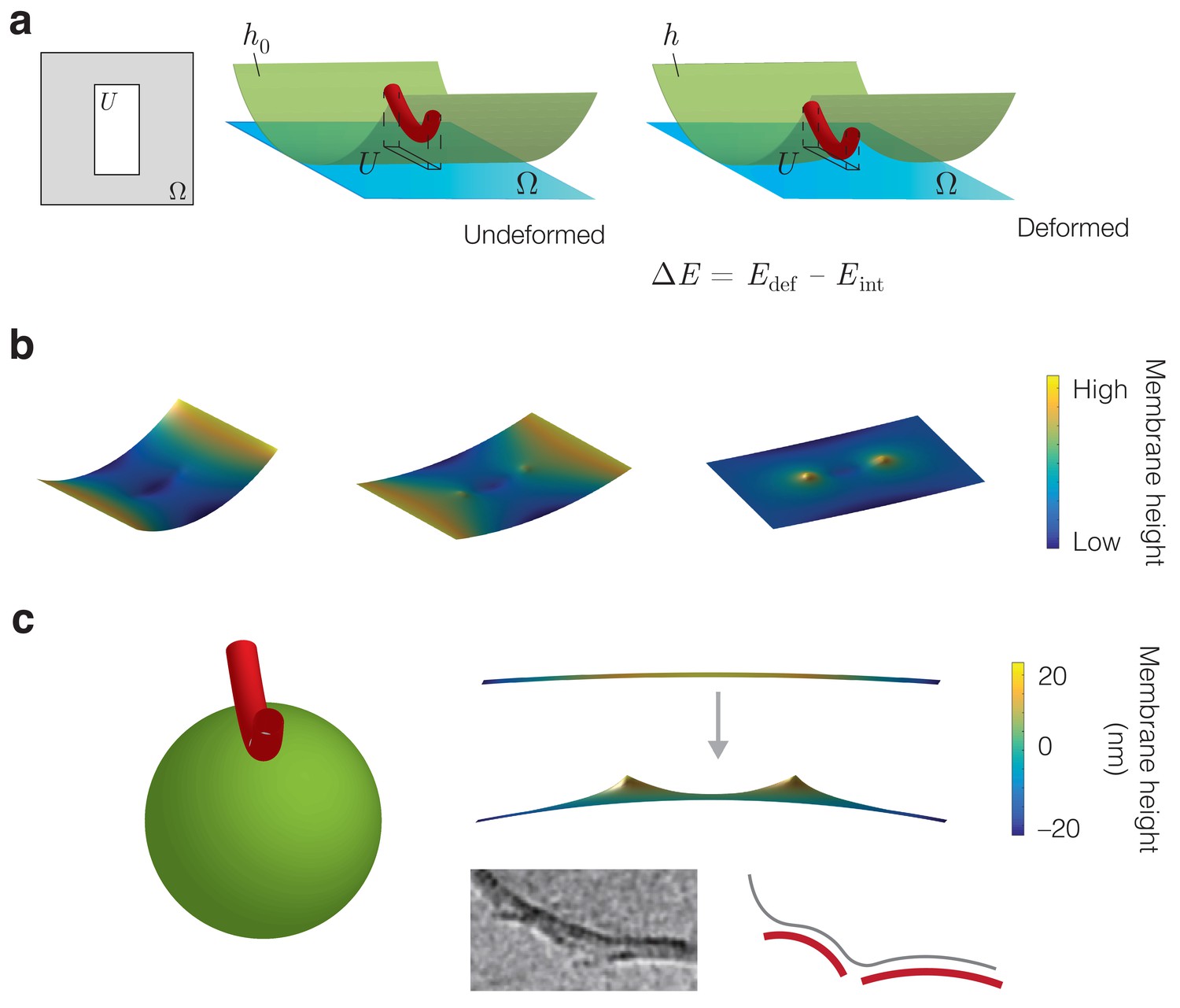
Energetic modeling of MreB binding and deformation of vesicles.

(a) A protein filament is modeled as a curved elastic rod that attaches to the inner membrane in an energetically favorable manner. $U$ denotes the interaction region. In the Monge gauge, a height function $h (x, y)$ parameterizes the membrane shape ( $h_{0}$ in the undeformed state) and the domain of $h$ ( $h_{0}$ ) is denoted $Ω$ . The interaction region restricts the value of $h$ over the region $U$ . (b) Example solutions for the membrane shape for $p = 0$ and $R_{c e l l} = 0.5 μ m$ , $1.5 μ m$ , and $\infty$ (left to right) on a finite domain, for the parameter values summarized in Supplementary file 1. (c) (Left) The binding of an MreB filament to a spherical vesicle induces vesicle curvature, a schematic of which is shown. (Right top) A numerical solution for the membrane shape over a finite domain where the undeformed configuration is a sphere with a principal curvature opposite that of an MreB filament. Here $p = 0$ , the sphere radius $R_{sphere} = 1 μ m$ , and the remaining parameter values are summarized in Supplementary file 1. (Right bottom) MreB filaments binding to vesicles in vitro, with a schematic shown. The image is reproduced here from Salje et al. (2011) under a CC BY 3.0 license (https://creativecommons.org/licenses/by/3.0/).

https://doi.org/10.7554/eLife.40472.005

Figure 3 with 3 supplements

Download asset Open asset

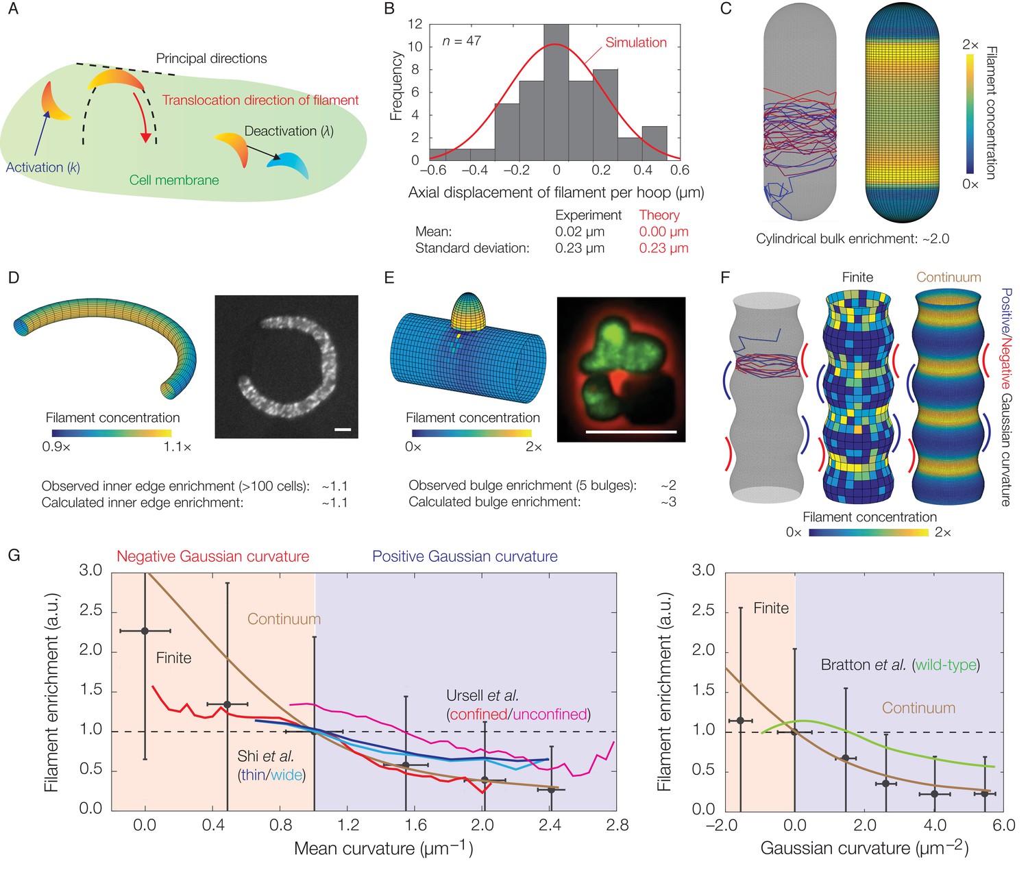
Dynamics of translocation and implications to MreB localization.

In this figure, the localization of MreB filaments, which exhibit a finite processivity and are assumed to follow the parameter values summarized in Supplementary file 2, is shown. (A) A schematic of the model of filament translocation. The filament is modeled as a point which moves processively in a direction determined by the principal curvatures. (B) Histogram of the axial displacements per hoop translocated of 47 MreB filaments in B. subtilis cells (Hussain et al., 2018), along with the theoretical prediction and a simulation result shown. (C) Langevin simulation (left) of Equation (3) and numerical result (right) for the filament concentration, $C_{F}$ , on a spherocylinder, for parameter values relevant to E. coli. Here and below, blue and red denote starts and ends of trajectories, respectively, details of simulations and numerics are provided in Appendix 1, and $C_{F}$ is found by solving the Fokker-Planck equation corresponding to Equation (3). (D) (Left) Numerical result for $C_{F}$ on a bent rod, for parameter values relevant to E. coli. (Right) Representative fluorescence microscopy image of an E. coli cell confined to a donut-shaped microchamber, with MreB tagged by green fluorescent protein (GFP), from Wong et al. (2017). The inner edge enrichment is calculated as described in Wong et al. (2017), and the scale bar indicates 1 μm. (E) (Left) Numerical result for $C_{F}$ on a cylinder with a bulge, for parameter values relevant to B. subtilis. (Right) Representative fluorescence microscopy image of a deformed B. subtilis cell with a bulge and GFP-tagged MreB, from Hussain et al. (2018). The bulge enrichment is calculated as a ratio of average pixel intensities, and the scale bar indicates 5 μm. (F) Langevin simulation and numerical results for $C_{F}$ on a cylinder with surface undulations in both the finite (Langevin, total of ~500 filaments) and continuum (Fokker-Planck) cases, for parameter values relevant to E. coli. (G) A plot of (left) the mean curvature and (right) the Gaussian curvature against filament enrichment for the figures shown in (F) (Langevin simulation, black; continuum case, brown), with empirically observed relations from confined and unconfined MreB-labeled E. coli cells (red and magenta) from Ursell et al. (2014), thin and wide mutant E. coli cells (blue and cyan) from Shi et al. (2017), and wild-type E. coli cells (green) from Bratton et al. (2018) overlaid. Error bars denote one standard deviation in the Langevin simulation, and 1 a.u. equals the mean of $C_{F}$ when the mean curvature is 1 µm⁻¹ (left) and when the Gaussian curvature is 0 µm⁻² (right). Note that the magenta and green curves are not normalized according to this convention.

https://doi.org/10.7554/eLife.40472.006

Figure 3—figure supplement 1

Download asset Open asset

Curvature-based translocation on cylinders with bulges.

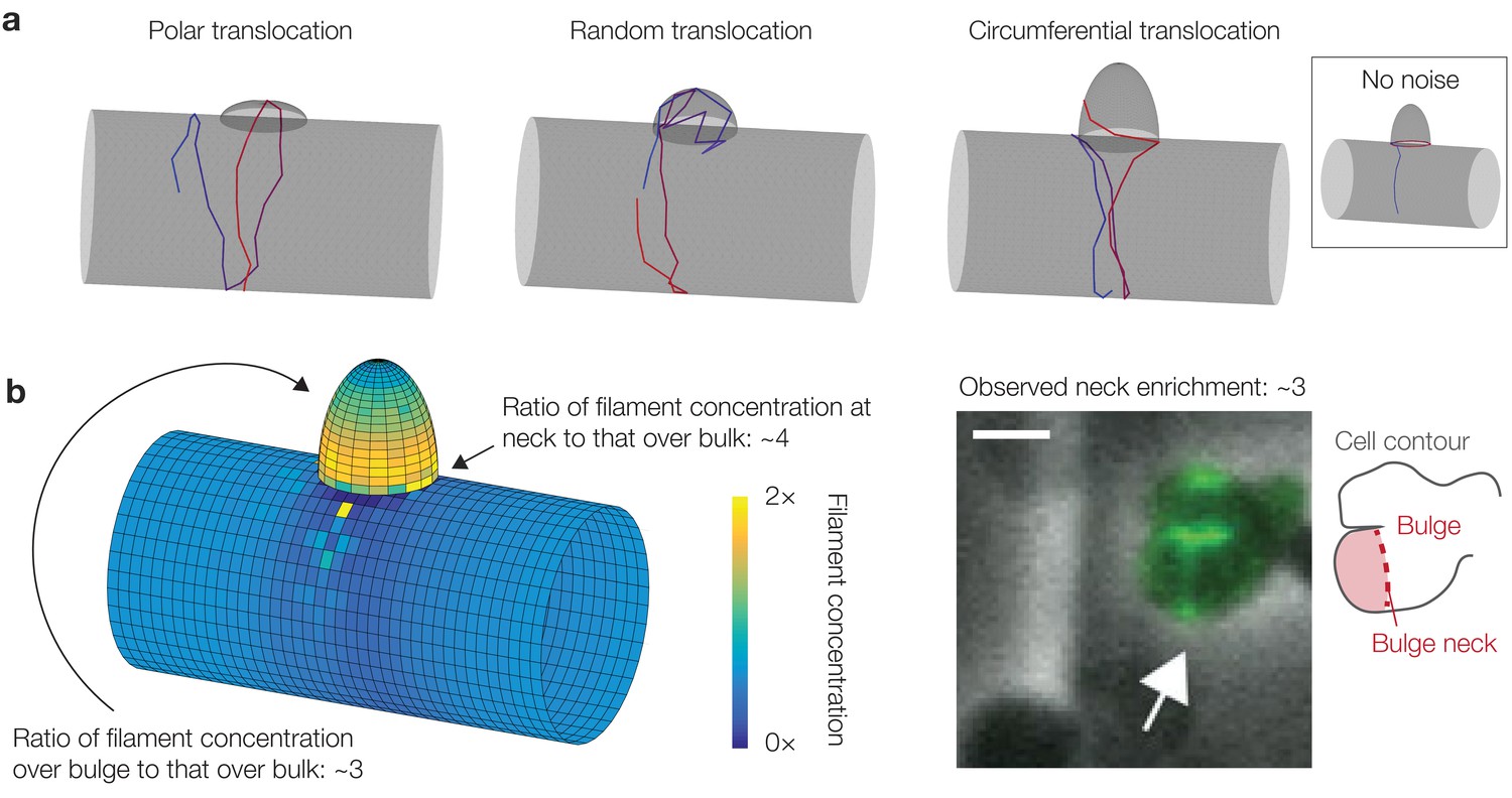
(a) Three different geometries corresponding to three different translocation behaviors, as summarized in §2.7 of Appendix 1. (b) Same as Figure 3E in the main text. Here $C_{F}$ is substantially increased at the bulge neck, with a magnitude consistent with previous experiments (Hussain et al., 2018). (Right) Microscopy image of a B. subtilis cell with a bulge and MreB filaments fluorescently tagged, from Hussain et al. (2018). The white arrow highlights the increased fluorescence intensity at a bulge neck, which is indicated by the schematic shown to the right. The scale bar indicates 1 μm.

https://doi.org/10.7554/eLife.40472.007

Figure 3—figure supplement 2

Download asset Open asset

Correlations between Gaussian and mean curvatures for, and translocation directions in, cylinders with undulations of different wavelengths.

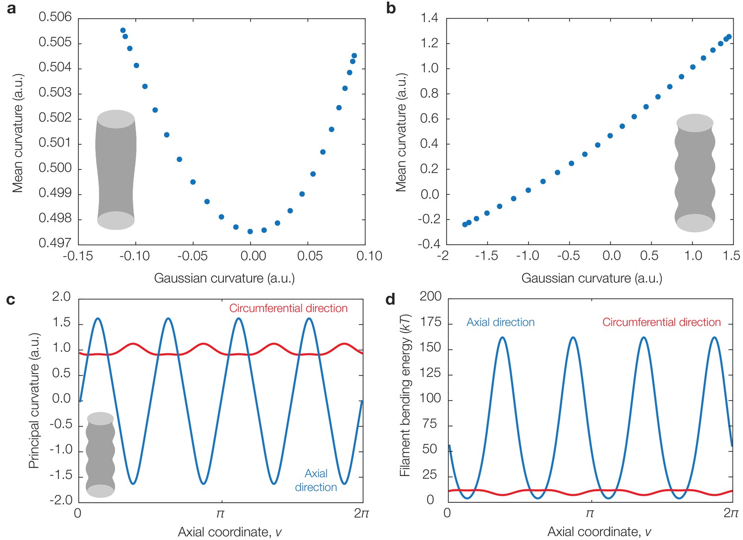
(a) Plot of sampled Gaussian curvatures against the corresponding mean curvatures for the geometry considered in §2.8 of Appendix 1 with $a = 1$ , $c = 0.1$ , and $P = 1$ . (b) Same as (a) but for $P = 4$ . (c) Principal curvatures corresponding to the geometry considered in (b). (d) Dimensionful bending energies of a filament aligning along each principal direction, for the parameter values summarized in Supplementary file 1, showing that, in this geometry as well, binding along the greatest principal direction generally incurs the least bending energy.

https://doi.org/10.7554/eLife.40472.008

Figure 3—figure supplement 3

Download asset Open asset

Effects of curvature-dependent translocation noise and varying filament properties on model predictions.

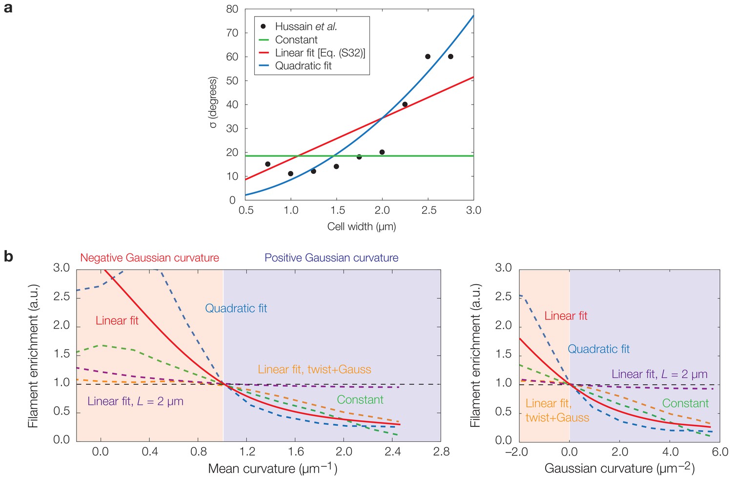
(a) Plot of experimentally observed median angles from the axis perpendicular to the cellular midline, taken to be identical to σ, against the cell width for B. subtilis cells of varying widths from Hussain et al. (2018). Curves corresponding to the assumptions of a constant σ, a linear fit $σ = α {(Δ c)}^{- 1}$ , and a quadratic fit $σ = β {(Δ c)}^{- 2}$ are overlaid, where the parameter values α and β are summarized in Supplementary file 2. (b) Same as Figure 3G of the main text, but with continuum limit predictions for the cases of a constant σ (green) and a quadratic fit $σ = β {(Δ c)}^{- 2}$ (blue), in addition to the case of a linear fit $σ = α {(Δ c)}^{- 1}$ (red) used in the main text. The continuum limit prediction for the case of a ten-fold larger filament step size, $L = 2 μ m$ , is also shown (purple), along with the prediction for the case of large twist and Gaussian curvature-dependent activation (orange; see also Figure 4—figure supplement 4h). Localization therefore arises for the different functional dependencies of σ on $Δ c$ shown in (a) and different filament properties.

https://doi.org/10.7554/eLife.40472.009

Figure 4 with 4 supplements

Download asset Open asset

Dependence of localization on processivity and Gaussian curvature.

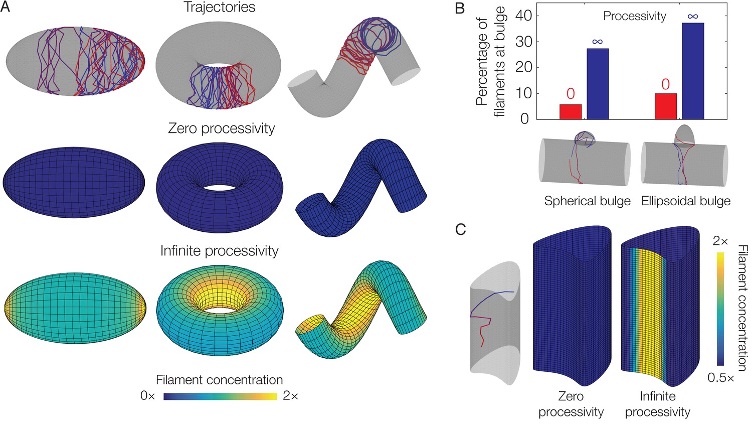
(A) Langevin simulations of Equation (3) and numerical results for $C_{F}$ , the filament concentration, on different surfaces. Note that cases of zero processivity correspond to uniform distributions and that we have considered the limiting cases of zero and infinite processivity, along with a constant value of the translocation noise ( $σ$ ), here. Figure 3 shows numerical results for the case of a large, but finite, processivity and a principal curvature-dependent translocation noise relevant to MreB. (B) Plot of the percentage of total filaments contained in a bulge, for the two different geometries indicated in the limits of zero and infinite processivity. (C) Langevin simulation and numerical result for $C_{F}$ on a non-circular cylinder in the limits of zero and infinite processivity.

https://doi.org/10.7554/eLife.40472.010

Figure 4—figure supplement 1

Download asset Open asset

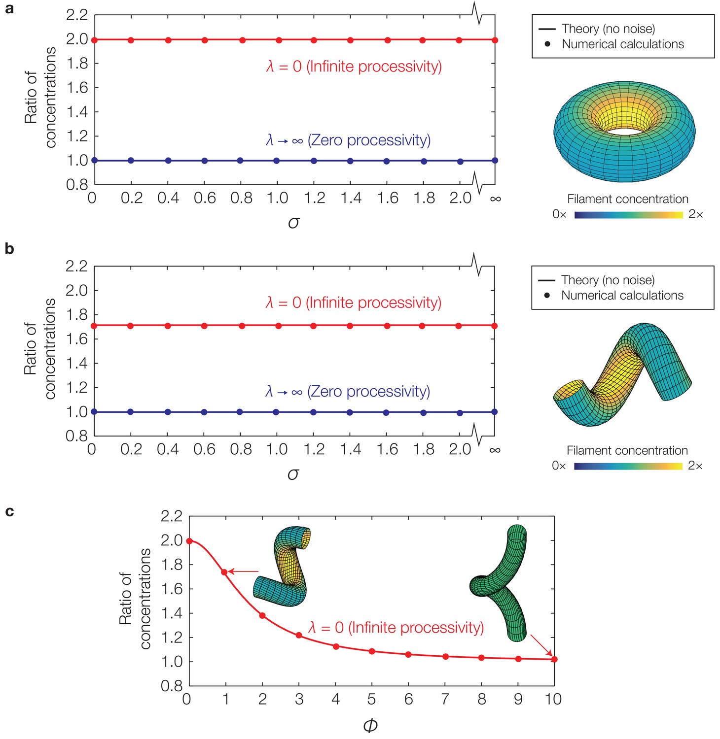
Curvature-based translocation on a torus and a helix.

(a) Plot of the ratio of $\int_{π}^{2 π} C_{F} 𝑑 u$ to $\int_{0}^{π} C_{F} 𝑑 u$ for a torus, corresponding to the ratio of filament concentrations between the inner and outer edges, against the translocation noise (σ), as determined by numerical calculations. The theoretical predictions assuming no noise are shown as lines. (Inset) Representative result for $C_{F}$ in the case of infinite processivity and $σ = 0.3$ , as shown with its zero processivity counterpart in Figure 4A of the main text. (b) Same as (a), but for a helix. (c) Same as (b), but against varying helical pitches ( $ϕ$ ) and for a fixed value of $σ = 0$ .

https://doi.org/10.7554/eLife.40472.011

Figure 4—figure supplement 2

Download asset Open asset

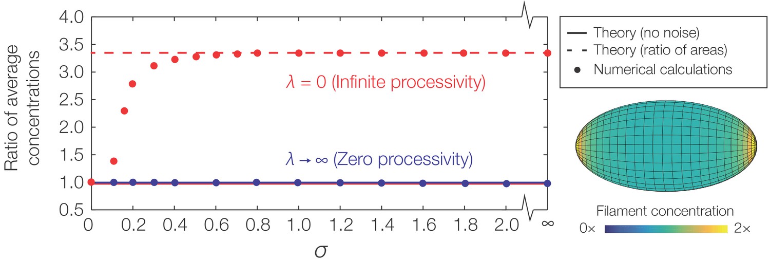
Curvature-based translocation on an ellipsoid.

Plot of the ratio of ${⟨ C_{F} ⟩}_{S}$ to ${⟨ C_{F} ⟩}_{S^{'}}$ , where $S = {X : u < π / 4 or u > 3 π / 4}$ denotes the caps and $S^{'} = {X : π / 4 \leq u \leq 3 π / 4}$ denotes the region away from the caps, against σ as determined by numerical calculations. The theoretical predictions assuming no noise are shown as lines. (Inset) Representative result for $C_{F}$ in the case of infinite processivity and $σ = 0.3$ , as shown with its zero processivity counterpart in Figure 4A of the main text.

https://doi.org/10.7554/eLife.40472.012

Figure 4—figure supplement 3

Download asset Open asset

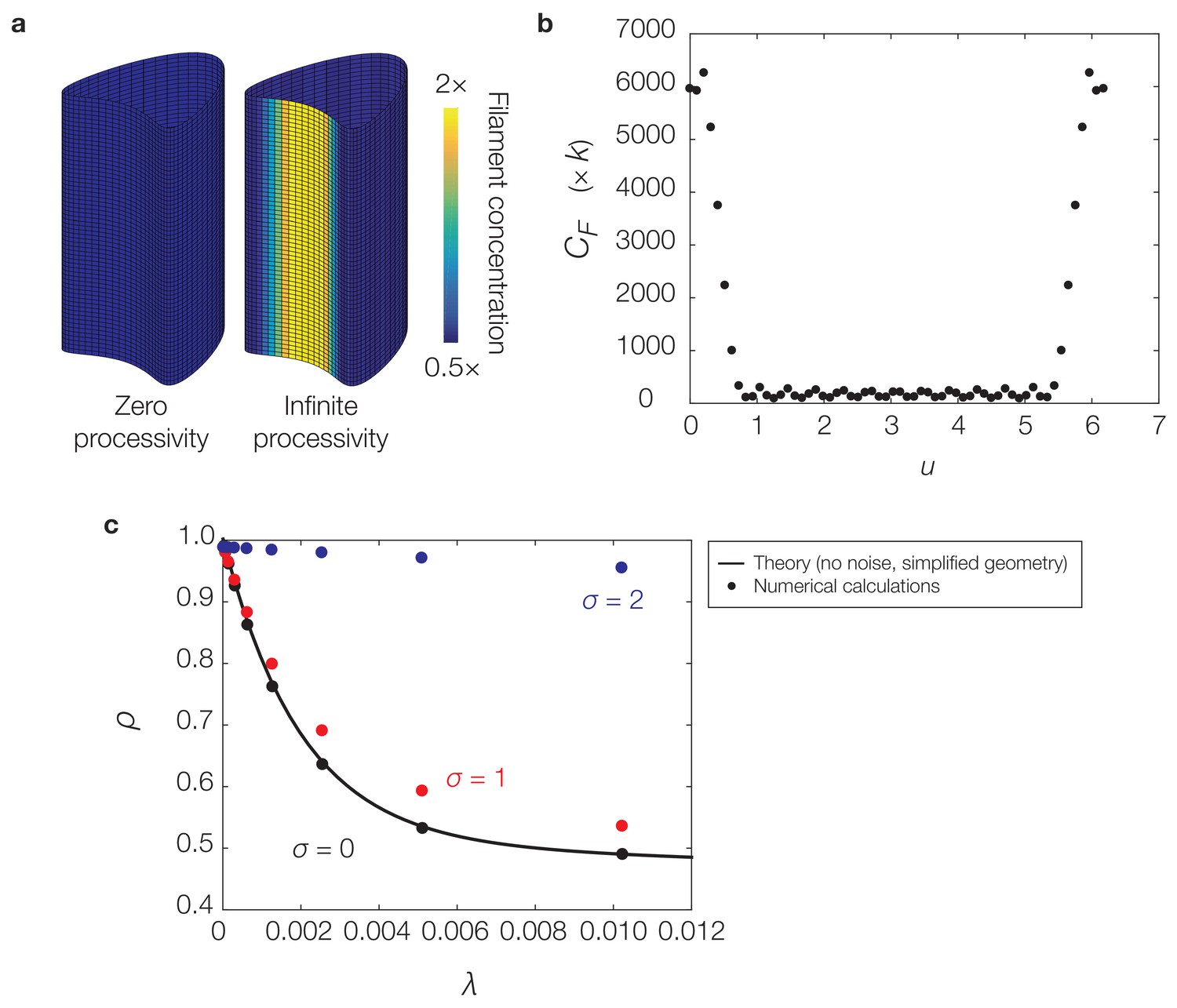
Curvature-based translocation on a geometry with zero Gaussian curvature.

(a) Same as Figure 4C of the main text. (b) Plot of the $u$ -coordinate against filament concentration, $C_{F}$ , (with units of $k$ ) for the case of infinite processivity in (a). (c) Plot of the deactivation rate, λ, against the localization ratio, $ρ$ , for similar calculations and parameters as in (a) but varying σ and λ. Similar to Equation (S31 ) of Appendix 1, $ρ$ is determined for the geometry considered here as the quotient $\max_{u} (N_{F} (u), λ) / \max_{u} (N_{F} (u), λ / 2)$ . The theoretical prediction for $ρ$ is determined in a simple case by Equation (S30 ) and (S31 ) of Appendix 1. For the theoretical prediction based on section 2.6 of Appendix 1, we set $ν = 0.4$ and $t = 10^{3}$ in non-dimensional units in the equations above to correspond to the values of $L$ and $N$ used in numerics.

https://doi.org/10.7554/eLife.40472.013

Figure 4—figure supplement 4

Download asset Open asset

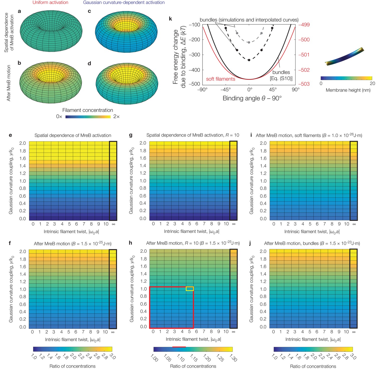
Effects of filament twist, flexural rigidity, and Gaussian curvature-dependent activation on model predictions.

(a-d) Numerical results for the filament concentration ( $C_{F}$ ) on a torus, for the parameter values relevant to E. coli as summarized in Supplementary file 2 and the absence (a, b) or presence (c, d) of Gaussian curvature-dependent activation, with $γ / k_{0} = 2$ (see also Figure 4—figure supplement 1). (e-j) Numerical results for the ratio of filament concentrations (see Figure 4—figure supplement 1) for a torus across different values of intrinsic filament twist, Gaussian curvature coupling, and flexural rigidity ( $B$ ). Panels (e), (f), (i), and (j), which all share the same color map, assume $R = 2$ while panels (g) and (h), which share the same color map, assume $R = 10$ , as to be comparable to curvatures observed in prior experiments (Wong et al., 2017). The black box indicates parameter values where filament binding becomes energetically unfavorable. The red box highlights the characteristic range of parameter values consistent with prior experiments (Wong et al., 2017) and estimates (Quint et al., 2016), while the corresponding red line highlights the calculated range of concentration ratios. The cell outlined in yellow indicates values simulated in Figure 3—figure supplement 3b. We find that the concentration ratios are largely robust to twist, but vary only for large values of Gaussian curvature coupling. (k) Similar to Figure 2B of the main text, but for numerical solutions of Equation (S6 ) of Appendix 1 for parameters relevant to E. coli—namely, a pressure of $p = 1 atm$ —and an MreB bundle with flexural rigidity $B = 1.5 \times 10^{- 23} J \cdot m$ , cross-sectional radius $r_{f} = 10 nm$ , and no twist over a domain size of $30 nm \times 240 nm$ (black points) and $40 nm \times 300 nm$ (gray points). One such solution, corresponding to a binding angle of $θ - 90^{\circ} = 0$ for the smaller domain, is shown to the right. The numerical results are similar to the estimate of Equation (S10 ) of Appendix 1 (black curve). The red curve and scale show the prediction of Equation (S10 ) of Appendix 1 for a MreB filament with $B = 1.0 \times 10^{- 26} J \cdot m$ and no twist.

https://doi.org/10.7554/eLife.40472.014

Author response image 1

Download asset Open asset

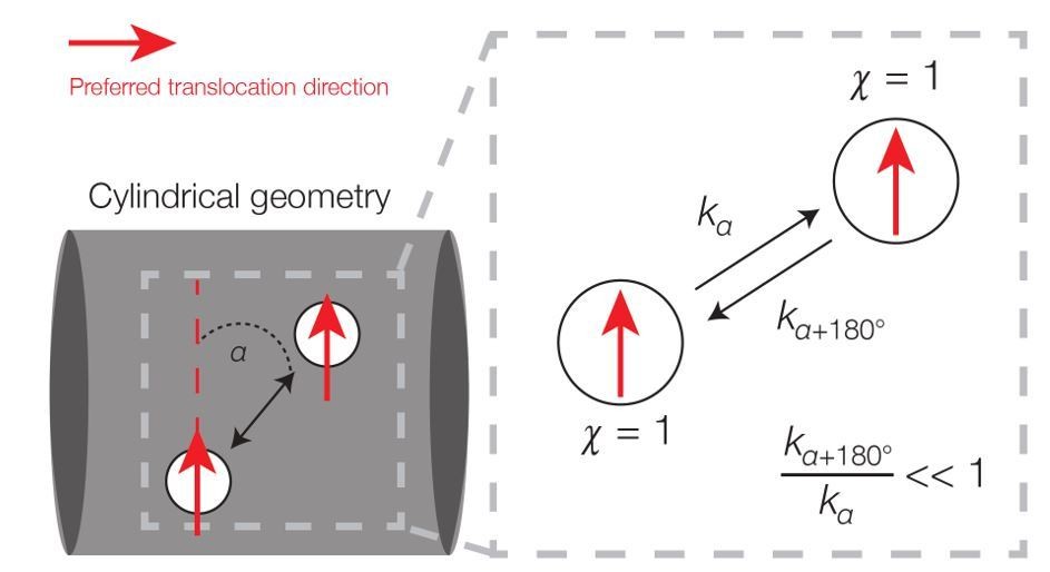
Broken detailed balance in translocation dynamics on a cylinder.

Here two area elements are separated by a distance L corresponding to the translocation step size. The red arrows indicate preferred translocation directions – that is, principal curvature directions oriented along the sign of χ_n. The corresponding dynamics (right) can be written, where k_α denotes the kinetic rate corresponding to translocation along a deviatory angle of α from the preferred translocation direction. For small α (α < 90°), the forward and backward rates are unequal because the probability of a filament reorienting to an angle of α+180° will be smaller than that of an angle α.

https://doi.org/10.7554/eLife.40472.020

Author response image 2

Download asset Open asset

In B. subtilis, the angular distribution of membrane-bound filaments within protoplasts confined to be rod-shape (protoplast filaments) is peaked at 90° relative to the long axis (mean deviation = 34°, n = 147), similar to that of MreB motion in wide (TagO-depleted), confined cells (mother machine tracks) (mean deviation = 36°, n = 359) and MreB motion in wild-type cells (Wt tracks) (mean deviation = 34°, n = 1041).

This figure is reproduced from Figure 3F of [Hussain et al., 2018] and adapted for the new Figure 1C of this work.

https://doi.org/10.7554/eLife.40472.021

Additional files

Supplementary file 1 Variables used, or calculated, in the model of filament binding and their numerical values.: https://doi.org/10.7554/eLife.40472.015
Download elife-40472-supp1-v2.pdf
Supplementary file 2 Variables used, or calculated, in the model of filament translocation and their numerical values for E. coli.: https://doi.org/10.7554/eLife.40472.016
Download elife-40472-supp2-v2.pdf
Transparent reporting form: https://doi.org/10.7554/eLife.40472.017
Download elife-40472-transrepform-v2.pdf

Download links

A two-part list of links to download the article, or parts of the article, in various formats.

Downloads (link to download the article as PDF)

Open citations (links to open the citations from this article in various online reference manager services)

Mendeley

Cite this article (links to download the citations from this article in formats compatible with various reference manager tools)

Felix Wong
Ethan C Garner
Ariel Amir

(2019)

Mechanics and dynamics of translocating MreB filaments on curved membranes

eLife 8:e40472.

https://doi.org/10.7554/eLife.40472

Sign up for email alerts

Privacy notice