Mechanisms of opening and closing of the bacterial replicative helicase
- City College of New York, United States
- The Graduate Center of the City University of New York, United States
- Simons Electron Microscopy Center, The New York Structural Biology Center, United States
- The Rockefeller University, United States
- Center for Excellence in Protein and Enzyme Technology, Faculty of Science, Mahidol University, Thailand
- Harvard University, United States
- CUNY Advanced Science Research Center, United States
Figures
Figure 1
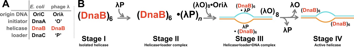
Initiation of DNA replication in bacteria and the assembly pathway for the replicative helicase.
(A) The four core molecular entities required for the initiation of DNA replication in E.coli and bacteriophage λ. The phage encoded ‘O’ and ‘P’ proteins recruit the host replication apparatus to drive replication from the phage Oriλ origin. The DnaB helicase participates in the initiation of DNA replication of both the chromosomal and phage genomes. (B) Prior work has defined at least four stages in the assembly pathway of the hexameric DnaB bacterial replicative helicase. Stage I features the isolated helicase. In Stage II, the helicase is captured by the helicase loader. In Stage III, the helicase • loader complex engages ssDNA at the origin, which is produced by the action of the initiator protein. In Stage IV, the loader has been expelled, and the helicase assumes an active conformation, which is competent to translocate along ssDNA.
Figure 2 with 6 supplements
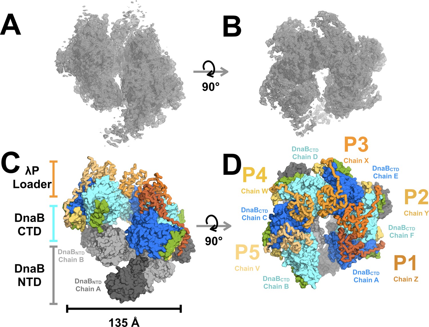
Architecture and stoichiometry of the E.coli DnaB helicase•bacteriophage λP complex.
(A) Experimental EM density map of the E. coli DnaB helicase•bacteriophage λP complex contoured at five sigma in PyMOL (see also Supplemental Figure 2—figure supplement 3). (B) Same as panel A except that the map has been rotated by 90°. (C) The E. coli DnaB helicase•bacteriophage λP complex is shown depicting the ruptured interface between DnaB subunits A and B and the deep canyon that runs through the complex. The complex has been sub-divided into three tiers: λP loader (individual chains are colored in shades of orange), the DnaB CTD (colored in alternating blue and cyan), and the DnaB NTD tiers (colored in alternating dark and light gray). The DnaB CTD-NTD linker helix (residues 182–202) is colored yellow and the DnaB CTD helix (residues 291–302),which is involved in λP-binding interactions, is colored green. (D) Same as panel C except that the model has been rotated by 90°. The five λP molecules in the complex are labeled λP1 (chain Z), λP2 (chain Y), λP3 (chain X), λP4 (chain W), and λP5 (chain V).
Figure 2—figure supplement 1
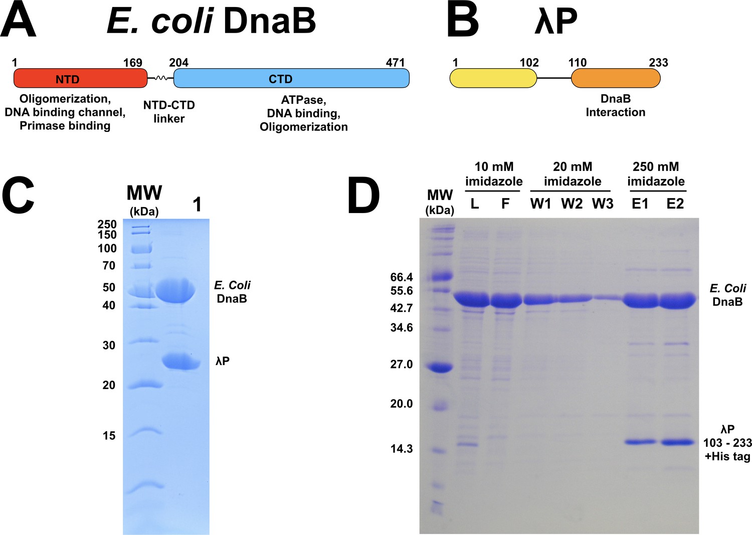
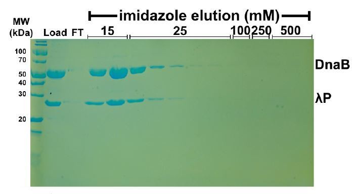
Architecture and biochemistry of the E.coli DnaB helicase and the bacteriophage λP helicase loader.
(A) Linear representation of the amino acid sequences of the E. coli DnaB helicase and (B) bacteriophage λ P helicase loader. The location of component domains is indicated. (C) SDS gel-electrophoretic analysis of the purity of co-expressed E. coli DnaB (52.4 kDa) and λP (26.5 kDa) complex (Lane 1). (D) SDS gel-electrophoretic analysis of NiNTA chromatography of the interaction between E. coli DnaB and a deletion construct of λP, which encompasses the carboxy-terminal 131 residues (λPΔ102-6xCHis (15.5 kDa). Co-expressed E. coli DnaB and λP- Δ102-6xCHis in 10 mM imidazole (L) was incubated with Ni-NTA beads; the beads were thrice washed with 20 mM imidazole (W1, W2, W3); purified DnaB • λP- Δ102-6xCHis after elution from the beads with 250 mM imidazole (E1, E2). Robust interaction between untagged DnaB and hexahistidine-tagged λP- Δ102 is clearly seen 1) from their co-elution in the presence of 250 mM imidazole and 2) failure of untagged DnaB to be retained on the NiNTA beads. Control expressions with an amino terminal construct of λP, encompassing residues 1–110, failed to express (not shown). Also, a control experiment to measure non-specific binding of the untagged E. coli DnaB • λP complex failed to show any interaction with the NiNTA beads (not shown).
Figure 2—figure supplement 2

Cryoelectron microscopy and cryoelectron tomography of the DnaB•λP helicase•helicase loader complex.
(A) Workflow associated with processing of single particle cryoEM (boxed in gray and yellow) and cryoET (boxed in blue) data, which resulted in the 4.1 Å map described above. Software used at each step in the workflow is indicated. The model that emerged from the cryoET procedure was used in two ways: 1) to generate projections for templates used to identify particles from EM images, and 2) as an initial model in the subsequent analysis of the identified particles. Details of this procedure and rationale can be found in the Appendix. (B) Cryo-electron tomography of the BP complex produced a low-resolution model with oblong dimensions and a prominent crack or canyon that extended throughout the length of the particle. (C) Projections using EMAN2 of the cryoET model in panel B provided low resolution two-dimensional templates for particle-picking. (D) The templates from panel C were used for template-based particle picking using Gautomatch. This procedure identified particles in our micrographs that manual and Gaussian-based efforts had been unable to distinguish from noise. The green circles on the top half of this micrograph represent particle coordinates identified by Gautomatch; the bottom portion of the same micrograph shows particle contrast. The white bar in the image signifies that although the underlying images arise from the same micrograph, the top and bottom halves of the image were generated independently (albeit with the same display values and contrast). (E) 2D class averages of a set of BP particles picked using Gaussian-based picking methods (left) and template-based picking methods (right). The Gaussian 2D class averages show high signal to noise ratios, however, subsequent calculation of a 3D structure was unsuccessful owing to the limited number of particle poses. 2D classification of a subset (~26,500) of the particles picked using the cryo-ET derived templates. These class averages showed high a signal to noise ratio and more diverse poses. In addition, high resolution details are now clearly visible. (F) Angular coverage of the BP map depicted in a 2D plot generated by Cryosparc.
Figure 2—figure supplement 3
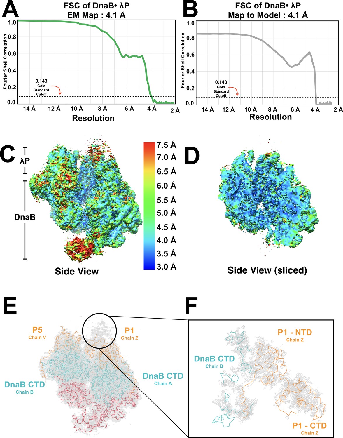
Quantitative analysis of the DnaB•λP EM density map.
(A) Fourier shell correlation of two independently refined half data sets indicates a global resolution of 4.1 Å, where the resolution is defined at the 0.143 gold standard (indicated by the black horizontal dotted line and labeled). (B) Fourier shell correlation (FSC) of the 4.1 Å BP map and the BP model. The FSC between our map and model was generated in Mtriage within Phenix. The resolution of the map to the model is also 4.1 Å as defined by the 0.143 gold standard (labeled and indicated with a black horizontal dotted line). (C) Local resolution estimates generated by ResMap and plotted onto the BP map in Chimera. The resolution of the entire particle falls within the 3.5–4.5 Å range. Lower resolutions are observed in the NTD of chain A and in the regions of weaker density above the λP1 helicase loader molecule (panels E and F). The local resolution estimates agree with the global resolution estimate as described and shown in panel A. Regions of density corresponding to DnaB and λP are indicated. The scale used to color the BP map is shown. (D) A sliced view of the map from Panel C shows local resolution estimates in the interior of particle. The sliced view of the particle is colored as in panel C. (E) The BP EM density map (gray mesh) shows additional, weaker, density adjacent to λP1 (chain Z). This map is contoured at a level of 4 sigma (PyMol). The NTD and CTD layers of DnaB are shown as ribbons and are colored red and blue, respectively. The λP tier is depicted in a ribbon view and colored in orange. (F) Model of the E. coli DnaB helicase • bacteriophage λP complex, which includes a 75 amino acid segment built into the less-well resolved regions of the density map. We tentatively assign this segment to the amino-terminal region of λP molecule λP1 (chain Z). We note that this segment appears to contact one of the DnaB subunits that lines the breached interface, and which is located at the top of the DnaB spiral. Strong density for DnaB chain B (teal) allows for visualization at a contour of 5 sigma and a carve setting of 2.0 Å. Visualization of the map at a lower contour of 3 sigma and a carve setting of 2.0 Å reveals weaker density for the NTD of protomer λP1 (orange). Density maps were visualized in PyMol.
Figure 2—figure supplement 4
3D classification of the DnaB•λP EM data.
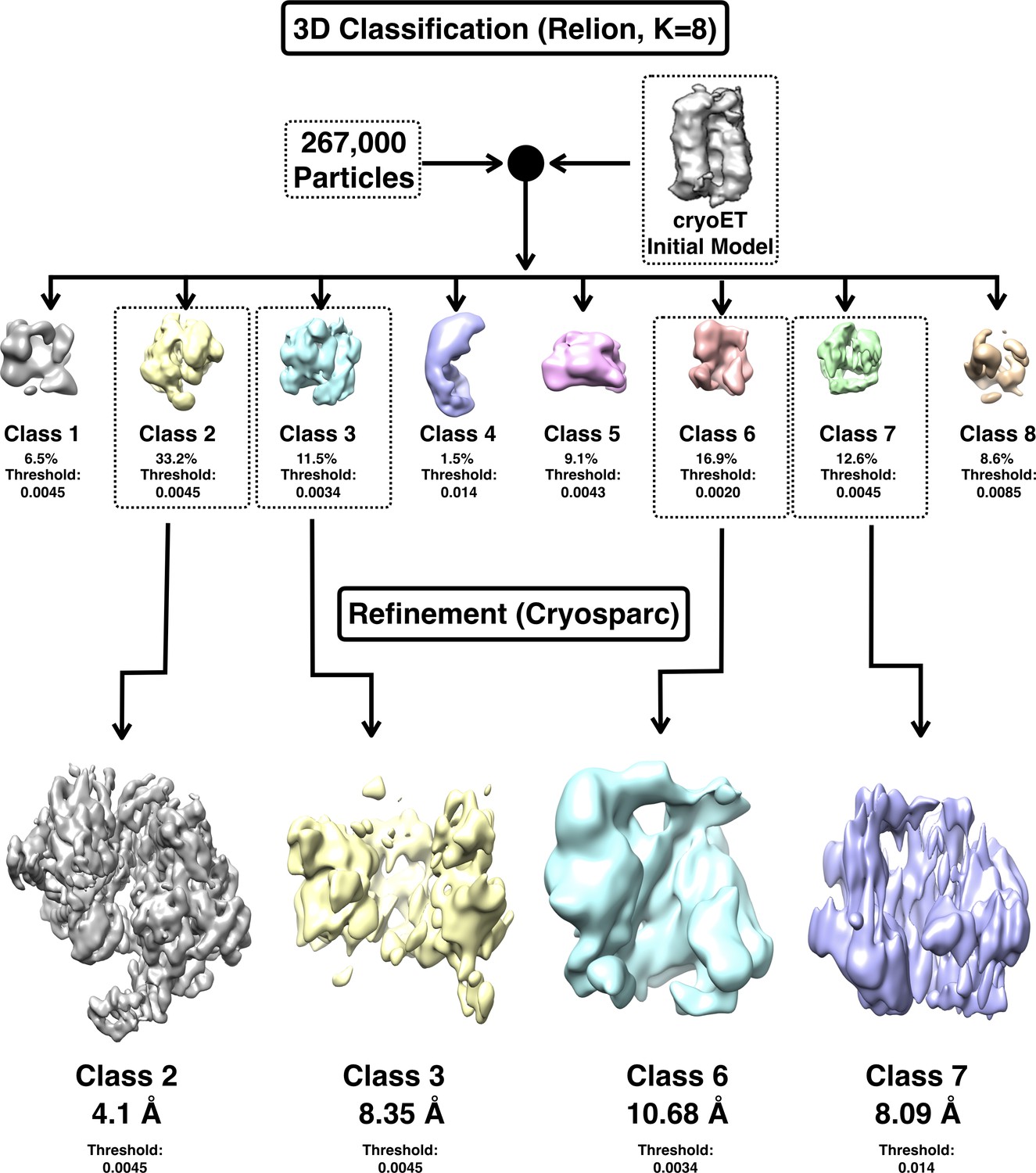
(A) 3D classification in Relion was used to sort all 267,000 particles into eight classes using the cryoET model as an initial model; this procedure served to clean the particle stack selected by means of template-based picking methods. Four of the classes (Boxed: Class 2, Class 3, Class 6 and Class 7) contained ~75% of particles and feature volumes of expected dimensions given our native MS measurements; these were autorefined to the indicated resolutions. The particles in class 2 were used to calculate the final 4.1 Å density map. The remaining four classes (Class 1, Class 4, Class 5 and Class 8) which accounted for ~25% of all particles contained particles of inappropriate dimensions to represent the BP complex; these were not used any further.
Figure 2—figure supplement 5

Interrogation of the DnaB•λP EM data set for additional stoichiometric or conformational states.
(A) Heterogeneous refinement (K = 6, Cryosparc) of all the particles used to calculate the 4.1 Å map was performed to determine if other BP stoichiometric or conformational states were present in our EM sample. This calculation produced a single class (colored in pale green and indicated with a red square) that could be attributed to the BP complex. The structure in this class corresponds to the DnaB6-λP5.entity; no other states were found. The volumes in Classes 1, 2 and 6 appear to be an open, planar form of DnaB. Classes 4 and 5 appear to be a distorted, open, non-planar DnaB, with no λP present. The percentage of particles in each class are indicated below the volumes. (B) Homogenous refinement (K = 6, Cryosparc) of all the particles used to calculate the 4.1 Å map. As with the heterogeneous refinement, only a single class with a volume corresponding to the BP complex was obtained (Class 3, shown in bright orange and indicated with a red square). This volume represents density corresponding to the DnaB6-λP5 species. The volumes produced by particles in Classes 4 and 5 show a DnaB architecture reminiscent of the BP complex, but they lacked density for λP. Classes 1, 2 and 6 yielded volumes that feature a distorted DnaB. (C) 2D classification (Cryosparc) of the particles used to calculate the 4.1 Å map. A small percentage (<1.4%) of these particles appeared to correspond to uncomplexed DnaB. Removal of these particles from our data set, followed by another round of refinement (Cryosparc), did not appreciably improve our EM map. The gold standard FSC curve (right) shows half-sets that converge at 4.1 Å. (D) Heterogenous refinement (using a single ab initio starting model) of all template-picked BP particles (~267,000) in Cryosparc yielded two classes of interest, both of which corresponded to DnaB6-λP5. One class, comprised of 29,734 particles, produced a map with a resolution of 8.02 Å, and a second class, with 84,647 particles, produced a map with a resolution of 7.25 Å. Although of lower resolution, these maps display comparable features as our 4.1 Å EM map.
Figure 2—figure supplement 6
Details of the atomic model and density of the DnaB•λP complex.
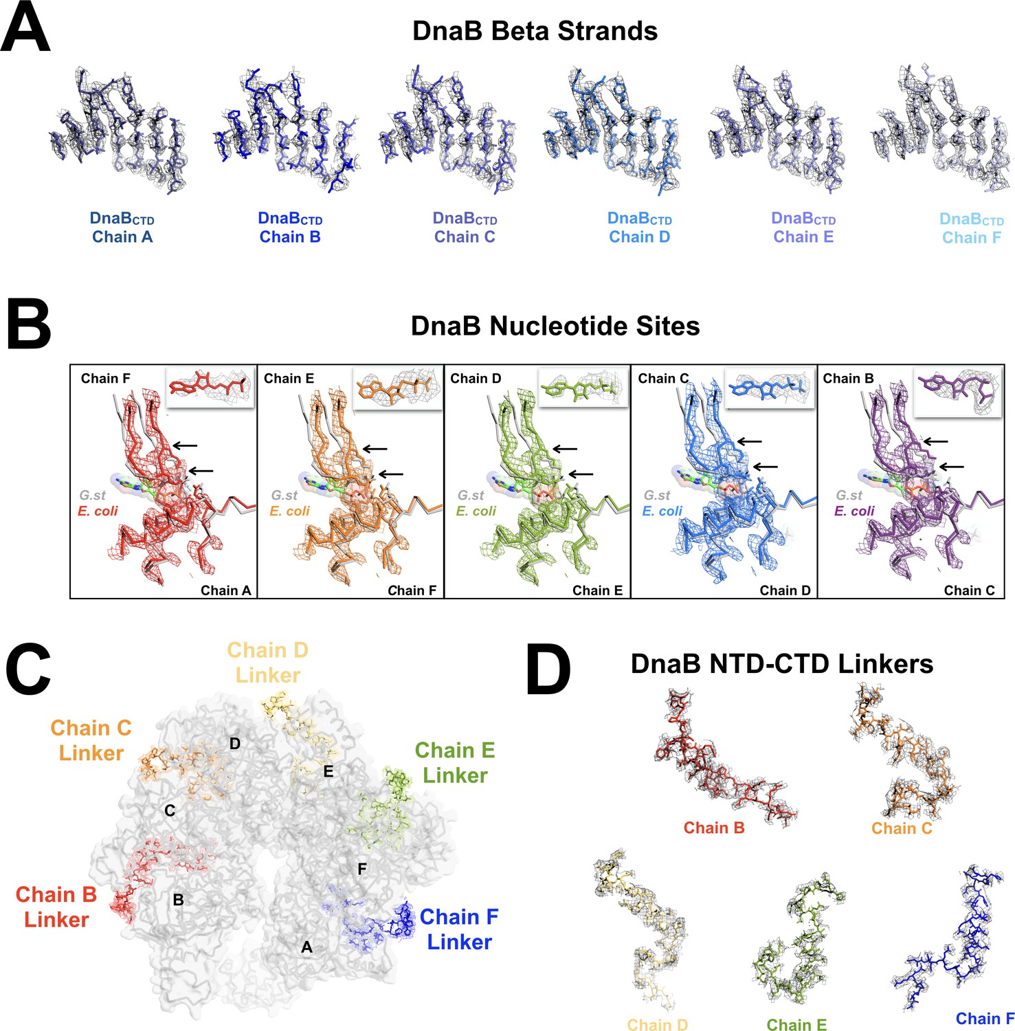
(A) EM density corresponding to the β-strands of the RecA fold of the C-Terminal domain of the DnaB helicase (residues shown: 226:232, 255:260, 309:313, 338:344, 378:384, 413:417 and 438:440). Density is shown at a sigma level of 6 (PyMol) and a carve of 2.0 for DnaB chains A (dark blue), B (bright blue), C (blue), D (marine), E (periwinkle) and F (light blue). Residues in the BP model are shown in ball and stick representation. (B) Superposition of each of the nucleotide-binding sites from the open spiral DnaB helicase (this work, E. coli) and the closed spiral ssDNA DnaB complex (PDB = 4ESV, G. st), as described in Figure 6B. The open spiral complex is depicted in gray ribbon for each. The nucleotide-binding site in the open spiral between chains A and F is depicted in red (panel 1); between chains F and E is depicted in orange (panel 2); between chains E and D is depicted in green (panel 3); between chains D and E is depicted in blue (panel 4); and between chains C and B depicted in purple (panel 5). Density is shown for residues 229:249, 257:276, 340:350 and 436:449 of the BP complex. Panels 1, 2, 3 and 5 include density at a sigma level of 8.0 and a carve of 2.0 Å in PyMol. The density in panel four is shown at a sigma level of 7.0 and a carve of 2.0 Å. Black arrows indicate the backbone shifts of two nucleotide-binding residues: K440 and R442. The GDP and aluminum fluoride from the closed ssDNA complex are depicted in ball and stick representation, with transparent spheres. Ball and stick representation is also used in the open spiral forms to depict residues implicated in nucleotide hydrolysis. All other components are shown in ribbon representation. The inset in each panel shows density in the BP map that we have modeled as ADP; the density corresponds to the chain being depicted. These density regions are shown in gray at a sigma level of 7 and a carve of 2.5 Å in PyMOL. The modeled nucleotide is shown in ball and stick representation and colored as the parent nucleotide site. (C) A top view of the DnaB helicase- λP helicase loader complex showing the position of the five DnaB N-terminal to C-terminal domain linkers (DnaB residues 168:202). Linkers are shown in stick representation with density displayed at a sigma level of 2 and a carve of 2.0 Å in PyMOL (chain B in red, chain C in orange, chain D in yellow, chain E in green and chain F in blue). Each DnaB CTD is labeled by chain. The rest of the BP complex is depicted in ribbon set within a surface representation and is colored gray. (D) Closeup representations of the quality of the density in the five NTD-CTD linkers of DnaB protomer chains B, C, D, E and F (residues 168:202) that we observed; density was not observed for the chain A linker. Density is shown at a sigma level of 2 and a carve of 2.0 Å in PyMOL and chains are colored as in panel C.
Figure 3 with 2 supplements
Stoichiometry and chain direction in the DnaB• λP complex.
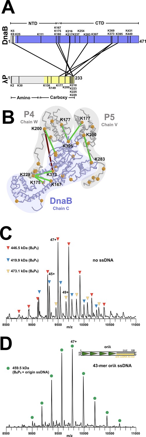
(A) Linear representations of the amino acid sequences of E.coli DnaB and λP colored in purple and yellow, respectively, to indicate the portions of each protein that are visible in our EM density maps. Architectural landmarks of each protein are indicated. The black vertical lines represent lysine residues. The black lines between DnaB and λP represent intermolecular crosslinks provided by the CX-MS procedure. Analysis of the BP complex using CX-MS appears in the Appendix section, in Figure 3—figure supplement 1 and in Table 2. (B) The CX-MS derived intermolecular crosslinks are plotted onto DnaB chain C, λP4 chain W, and λP5 chain V of the BP model. All lysine residues are depicted as orange spheres. Lysine residues reported by CX-MS to have been crosslinked are numbered. Lysine residues connected by a line are those which were detected by the CX-MS procedure (Table 2). Colored in red is the sole lysine pair whose distance exceeds 30 Å; the other lines capture distances below 30 Å and are colored in green. The various chains of DnaB and λP are outlined. (C) Native MS analysis of the E. coli DnaB helicase•bacteriophage λP complex. The most intense peak series corresponds to the B6P5 assembly, with lower relative intensity peaks indicating presence of subpopulations of B6P4 and B6P6. Notably, the mass estimates indicated that no nucleotide was present in any of the three populations of the BP complex, which is distinct from that seen in the native MS of Aquifex aeolicus DnaB-DnaC in which five nucleotides were observed (Figure 8—figure supplement 1). (D) Incubation of the DnaB•λP sample from panel C with a lambda replication origin-derived 13.1 kDa 43-mer ssDNA yielded a single peak series with a mass corresponding to the B6P5 assembly with one bound origin-derived ssDNA molecule. As with the samples without ssDNA (panel 3C), the mass estimates indicated that no nucleotide was present in the ssDNA complex. The inset depicts the oriλ replication origin and shows the location of the 43-mer DUE-derived ssDNA (Learn et al., 1997) used in this experiment.
Figure 3—figure supplement 1
Cross-linking mass spectrometry of the DnaB•λP complex.
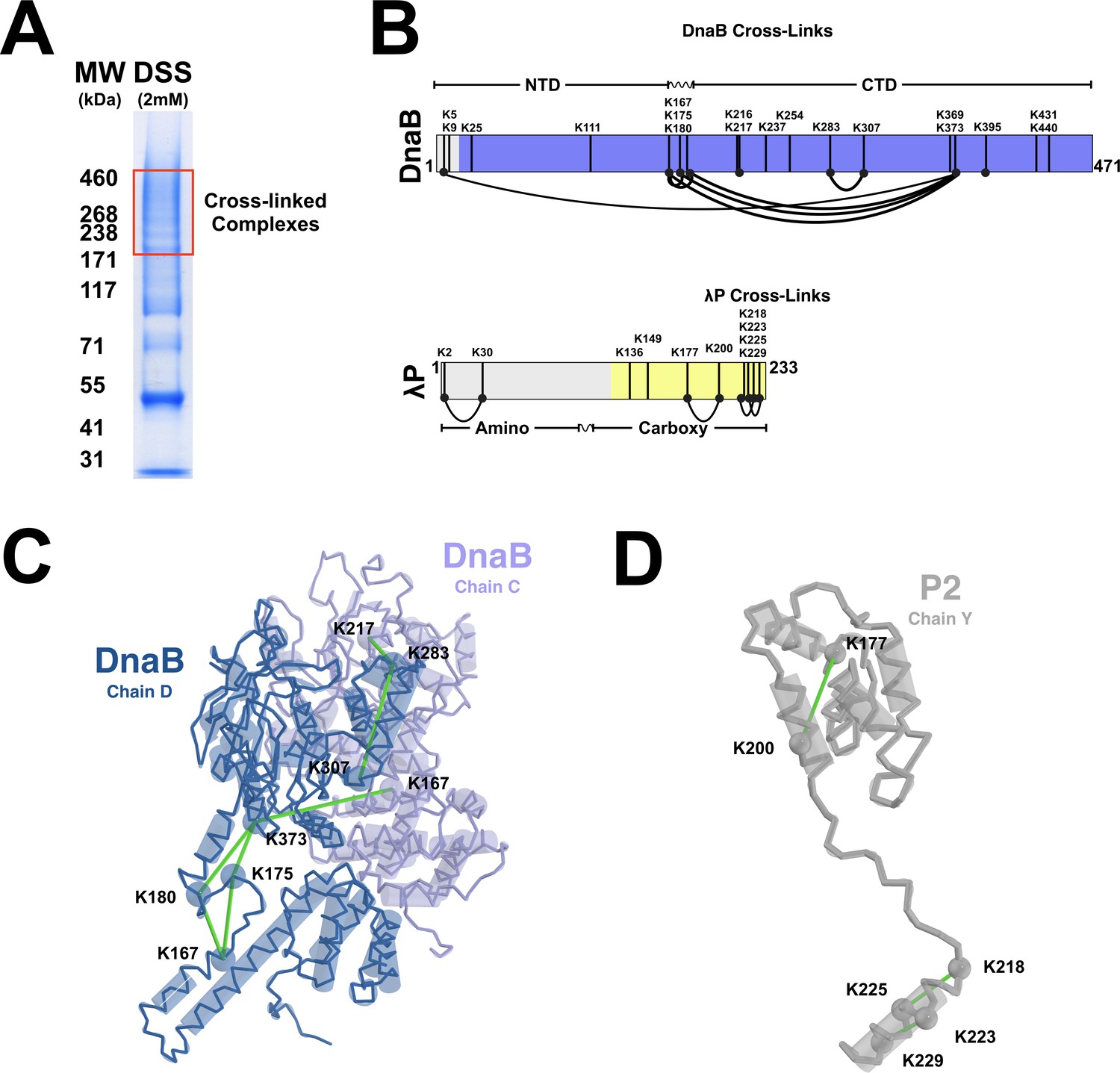
(A) SDS-PAGE gel electrophoretic analysis of crosslinking of the BP complex by the DSS crosslinking agent. The boxed region (red), containing cross-linked BP, was excised from the gel, digested with trypsin, and analyzed by MS as described in the Materials and methods. (B) DnaB and λP cross-links detected by CX-MS are plotted onto a linear representation of the amino acid sequence of E. coli DnaB and λP. Component domains and the linker segment are indicated. The purple and yellow colors represent portions of DnaB and λP, respectively, that are visible in our density maps; colored in gray are regions that are not visible. The black vertical lines represent lysine residues in the sequence. The curved black lines represent pairs of lysine residues reported to be crosslinked by the CX-MS procedure. We note that CX-MS is silent on whether these crosslinks arise from intra or intramolecular interactions, thus, for simplicity we represent them here as intramolecular crosslinks. (C) Intermolecular and intramolecular DnaB crosslinks plotted onto DnaB Chain C (purple) and DnaB Chain D (blue) of our model. The alpha carbons of lysine residues involved in cross-links are shown in spheres, and cross-links are shown as green lines between lysine residues. Distances captured by the green lines are less than 30 Å, and, thus, are consistent with the CX-MS data. Additional details appear in Table 2. (D) λP crosslinks plotted onto λP2 (chain Y), rendered in the same fashion as panel C. Additional details of our CX-MS study appear in Table 2.
Figure 3—figure supplement 2

Native MS of DnaB•λP with ssDNA.
(A) Native MS spectra of isolated BP are shown before and after incubation with a series of thymidylate homopolymers of varying nucleotide lengths (e.g. 25, 35 and 45). The measured masses reveal that none of the homopolymers were bound by the BP complex. By contrast, mass measurements of BP complex in the presence of origin-specific ssDNA (see also Figure 3D) provide evidence for a complex between BP and oriλ derived ssDNA.
Figure 4
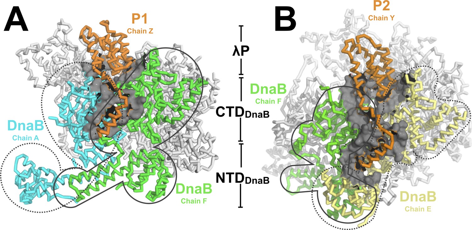
The DnaB•λP complex features two types of interfaces.
(A) An example of the first type of interface in the BP complex occurs between λP1 (chain Z, orange) and chain A (cyan) and chain F (light green) of DnaB. Other DnaB chains are colored in white. The surface representation (gray) includes DnaB residues within 10 Å of an alpha carbon from λP1 (chain A: residues 232, 278–306, 387–395, 419–432, 454–457; chain F:182–203, 213, 214, 217, 388–403,419-421, 429–439, 445–450, 463–468). This interface includes only contacts to the DnaB CTDs of the above chains. The BP complex includes three instances of this type of interface (to λP protomers: λP1, chain Z; λP3, chain X; and λP5, chain V). (B) A second type of interface in the complex is comprised of λP2 (chain Y, orange) and chain F (light green) and chain E of DnaB (light yellow). Other DnaB chains are colored in white. The surface representation (gray) includes positions in either of the above chains of DnaB that come within 10 Å of λP2. In this second type of interface, λP makes contacts to the CTD and NTD of the above DnaB chains. The BP complex includes two instances of this type of interface (to λP protomers: λP2, chain Y; and λP4, chain W).
Figure 5 with 1 supplement
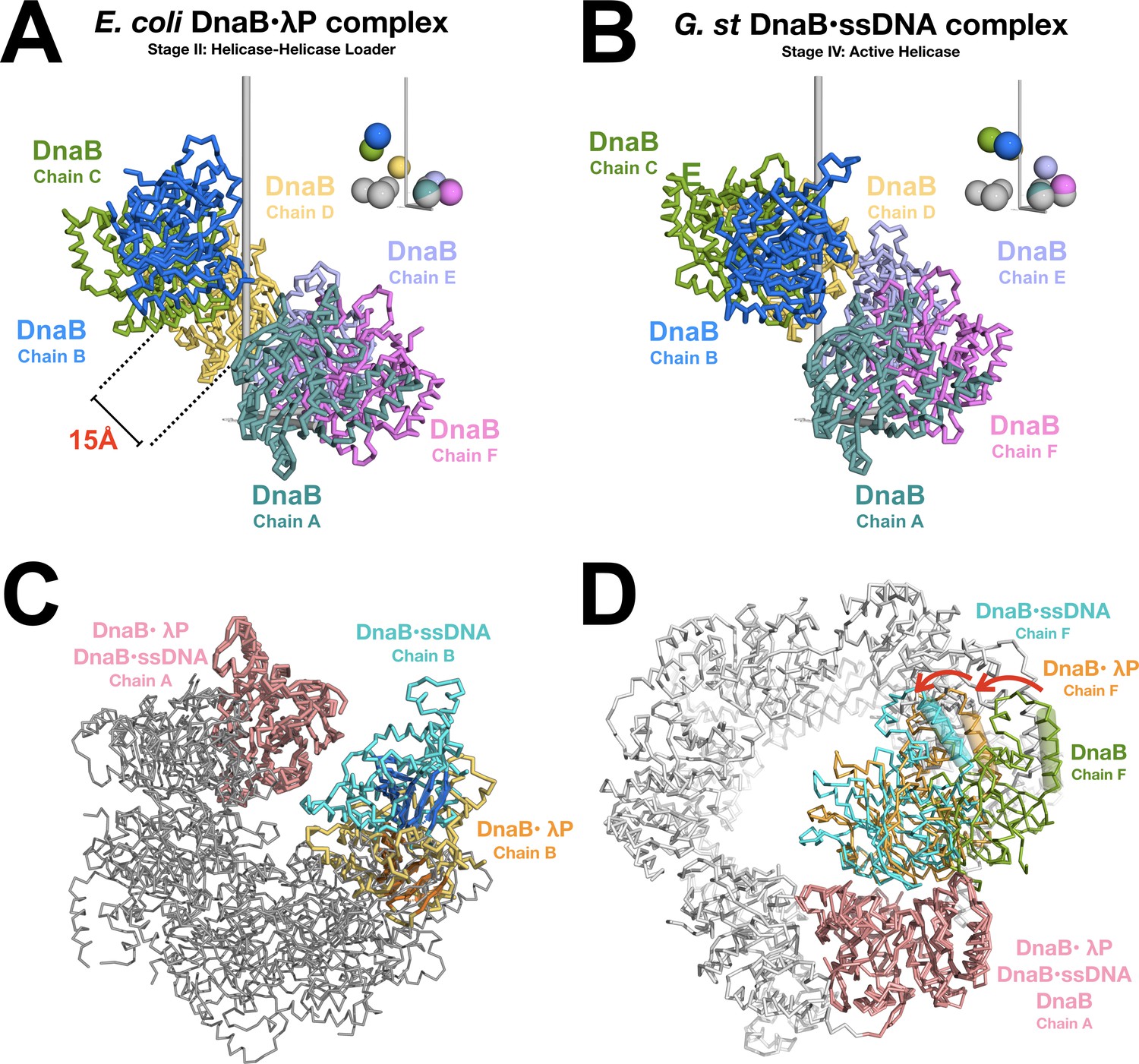
Opening and closing of the CTD tier of the DnaB helicase.
(A) The CTD layer in the DnaB helicase in the BP complex adopts a right handed pseudo-helical configuration after the transition from the closed planar (PDB = 4NMN) to the open spiral form of the BP complex. The CTD layer exhibits a pitch of ~16 Å. DnaB from the complex is depicted in a ribbon representation, colored by subunit and labeled by chain. The inset shows colored spheres drawn at the center of mass of each CTD using the same color as the associated subunit. The gray spheres in the inset represent centers of mass for CTDs from the closed planar constricted form of DnaB (PDB = 4NMN). The pseudo-helical axis is aligned with the vertical axis, which is shown in gray. (B) Same as panel A except that the CTD layer from the DnaB helicase in the ssDNA complex (PDB = 4ESV) is shown. The 4ESV CTD layer adopts a pitch of ~27 Å. DnaB from the ssDNA complex is depicted in a ribbon representation, colored by subunit and labeled by chain. As in panel A, the inset shows colored and gray spheres drawn at the centers of mass of each CTD from DnaB in the ssDNA complex and the closed planar constricted form (PDB = 4NMN), respectively. (C) Closing of the CTD tier is inferred from comparison of the open spiral in the BP complex to the closed spiral form of the ssDNA complex (PDB = 4ESV). The DnaB helicase from the BP complex and the ssDNA complex are superimposed on subunit A (both colored pink). Subunit B, which lines the ruptured interface in the BP complex is colored orange. The beta sheets of the RecA style fold are shown in a cartoon representation. The corresponding subunit in the closed spiral ssDNA complex is colored cyan. The remaining DnaB subunits are colored gray. (D) Inclination of individual subunits of DnaB towards the helical axis during opening and closing of the helicase. The open spiral BP complex (orange), the closed spiral ssDNA complex (blue, PDB = 4ESV), and the closed planar dilated form (green, PDB = 2R6A) are superimposed on subunit A of the DnaB helicase (pink). Changes in the relative orientation of subunits were calculated by measuring the degree of rotation of the next subunit (chain F) in the helicase. One structurally conserved CTD helix (residues 293–305 of BP, residues 272–284 of the closed spiral ssDNA complex and residues 271–285 of the closed planar dilated form) is indicated by a cylinder. Other subunits in the closed planar dilated form (PDB = 2R6A) structure are colored white.
Figure 5—figure supplement 1
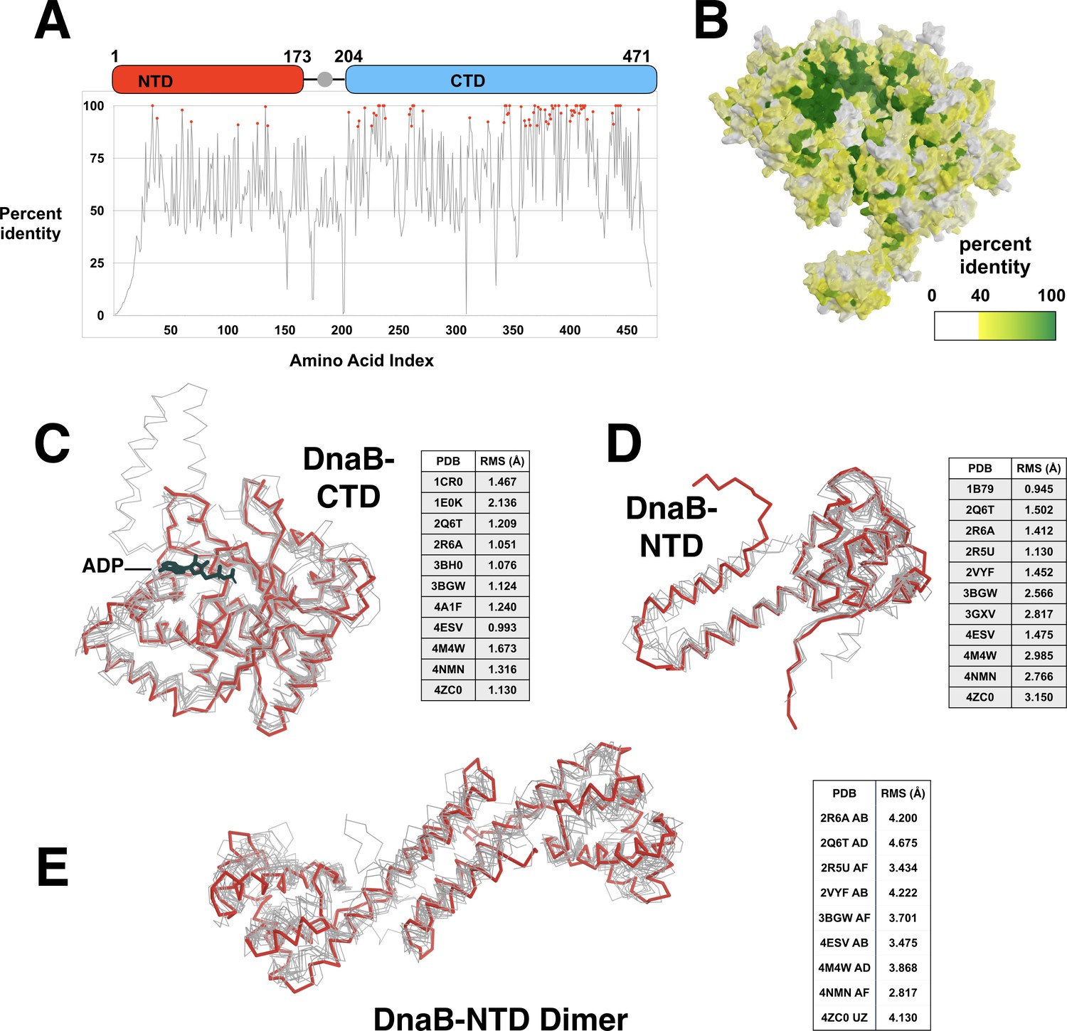
Conservation of the amino acid sequence and structure of the DnaB helicase.
(A) Sequence similarity of the TIGR00665 conserved protein domain family is plotted against the amino acid sequence of E. coli DnaB helicase, one member of this family. The domain architecture of DnaB is superimposed on the plot. (B) The sequence similarity data in panel A is projected onto the surface of the DnaB portion of the BP complex. The surface is colored from white (identity of 0–39%) to a gradient of yellow (identity of 40%) to dark green (similarity of 100%). (C) Eleven instances of the CTD of the DnaB helicase (colored in gray) are superimposed on the CTD (residues 204:468) of DnaB in the BP model (colored in red). For reference, a single ADP molecule marks the site of the nucleotide-binding site. The high structural conservation is indicated by the low RMSD values in the inset table. (D) Eleven instances of the NTD of the DnaB helicase are superimposed on the NTD (residues 1:173) of DnaB in the BP model. As with the CTD, structural conservation of the NTD is high. This figure is colored as in panel C. (E) NTD dimers from nine structures superimposed onto a monomer of an NTD dimer from the BP complex (residues 1:173). Global alignment indicates structural conservation of the NTD dimer. The various structures used in the above calculations are indicated by PDB entry. In panel E, the chain identifiers of the respective NTD dimers are indicated in the adjacent table. This figure is colored as in panel C.
Figure 6
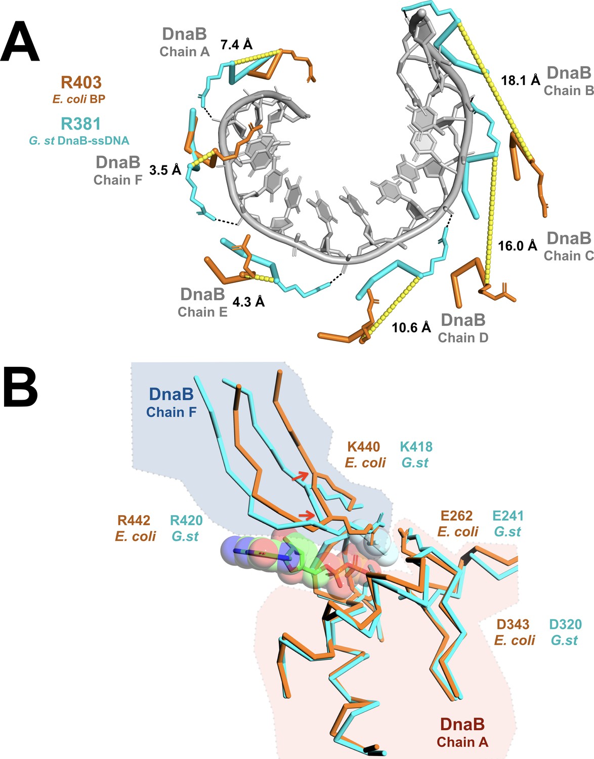
Remodeling of the CTD tier shifts the ssDNA binding and ATP hydrolytic sites into inactive configurations.
(A) The effect of remodeling of the CTD tier by λP is seen in the misalignment of the DNA-binding residues in the BP complex when compared to the ssDNA complex. In the ssDNA complex, three side chains (G.st: R381, E382, G384; E. coli: R403, E404, G406) from each DnaB protomer contact two consecutive phosphate groups; for clarity, only R381/R403 are shown. In the BP complex, the altered positions of these residues distorts the binding site, which may preclude interactions with ssDNA. The DnaB portions of the BP and ssDNA complexes were superimposed on chain A of DnaB. The ssDNA component from the translocating DnaB helicase structure (PDB = 4ESV) is depicted as a gray cartoon, and amino acids that contact the phosphate backbone are shown as sticks and colored in cyan (G.st, ssDNA complex) or orange (E. coli, BP complex). Distances between the α-carbon of the corresponding residues in the BP and ssDNA bound complexes are indicated and marked with a yellow dashed line. The approximate position of each chain of DnaB is also indicated. (B) Superposition of the nucleotide-binding sites from the open spiral (this work, colored orange) and the closed spiral ssDNA complex (PDB = 4ESV, colored cyan). The catalytic glutamate (E262) of the BP complex is sub-optimally positioned for hydrolysis, as are the α-carbons of the two nucleotide- binding residues: K440 and R442 (indicated with red arrows). The GDP and aluminum fluoride from the closed spiral ssDNA complex are depicted in a ball and stick representation, with transparent spheres. Amino acid residues in DnaB implicated in hydrolysis are shown in a ball and stick representation. Other parts of the DnaB helicase are depicted in ribbon representation. A complete presentation of the nucleotide-binding sites appears in Figure 2—figure supplement 6.
Figure 7

Remodeling of the NTD tier of the DnaB helicase by the λP helicase loader.
The NTD layers from the various stages of the helicase assembly pathway are compared. Three types of contacts between the NTDs of DnaB monomers have been described among the various forms of DnaB: tail-to-tail (colored in magenta), head-to-tail (colored in blue), and head-to-head (colored in orange). Residues within 4 Å across a particular interface are colored. Head refers to the globular domain in the NTD (A. aeolicus: 8–109, E. coli: 32–123, G. stearothermophilus: 1–112) and tail refers to a pair of helices that comprise a helical hairpin in the NTD (A. aeolicus: 110–149, E. coli: 124–173, G. stearothermophilus: 113–151). The top set of images is rotated by 90° relative to the bottom images. (A)The NTD layer (PDB = 4NMN) from the constricted closed planar configuration in Stage I of the helicase assembly pathway. (B)The NTD layer from the BP complex. Binding of the λP helicase loader to DnaB reconfigures the NTD layer into an open spiral; reconfiguration breaches one of the head-to-head interfaces to create a ~ 20 Å opening. The NTD layer from the BP complex adopts the constricted configuration as defined by the width of the central chamber. (C)The NTD layer from the ssDNA bound form of DnaB (PDB = 4ESV). This NTD layer adopts an open spiral configuration wherein one head-to-head interface is disrupted. Unlike the BP the complex, however, the central chamber in the ssDNA complex is topologically closed through interactions between the NTD and CTD tiers (not shown). The NTD layer is found in the dilated configuration.
Figure 8 with 2 supplements
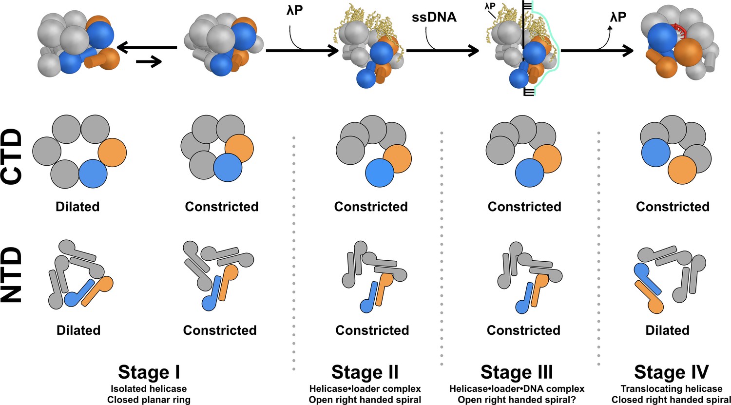
Model for assembly of the bacterial DnaB replicative helicase at the origin of DNA replication.
The overall structure and conformational state of DnaB in the four stages of the assembly pathway are schematically depicted to include insights from this work. The structure of DnaB is depicted in cartoon form with spheres drawn in place of each CTD and a sphere/cylinder in place of each NTD globe/helical hairpin tail. Each subunit is colored gray, except for the Stages I, II, and III chains A and F, which are shown in blue and orange, respectively. In the Stage IV model, chains A and B are colored orange and blue, respectively. The five copies of the λP helicase loader are depicted as yellow ribbons. A two dimensional representation of the configuration of each tier in the various stages is drawn below each cartoon, colored in the same way. In Stage I of the assembly pathway, DnaB is found in equilibrium between two conformers, termed dilated and constricted. This distinction applies to both the NTD and CTD layers. Addition of the λP helicase loader results in a conformational change in DnaB in which the CTD and NTD tiers are ruptured (Stage II); in this stage, both the CTD and NTD tiers adopt the constricted configuration (this work). In Stage III, the helicase•helicase loader complex engages ssDNA and the initiator protein (not shown) at the oriλ replication origin (produced by prior action of the initiator protein, not shown). Little is known about the path of ssDNA through the complex, as such, it is modeled as a simple cartoon. It is anticipated that both the NTD and CTD tiers in Stage III will retain the constricted configuration of Stage II. Expulsion of the loader protein accompanies transition to Stage IV of the pathway. The CTD layer closes and remains in the constricted conformation. The NTD layer is also sealed, however, its configuration assumes the dilated conformer.
Figure 8—figure supplement 1

Comparison of bacterial helicase•helicase loader complexes.
(A) Native MS analysis of the DnaB-DnaC complex from A. aeolicus. A single peak series at high m/z range was observed. The mass calculated from this peak is 485,290 ± 30 Da and corresponds to a B6C6 assembly and five nucleotides. We note that the peaks within the series are broad indicating adduction and/or heterogeneity. The measured mass is within 0.3% of the expected mass of B6C6. (B) The structures of various bacterial helicase•helicase loader complexes are shown. E.coli DnaB•λP (left), 25 Å EM map of the E. coli DnaB6•DnaC6 complex (center), and G.stearothermophilus DnaB6•G.subtilis DnaI6•DnaG6 (right). Comparable helicase protomers for each complex are colored using the same color. The λP helicase loader is colored orange, the region corresponding to DnaC is colored in peach and DnaI is colored in dark green.
Figure 8—figure supplement 2
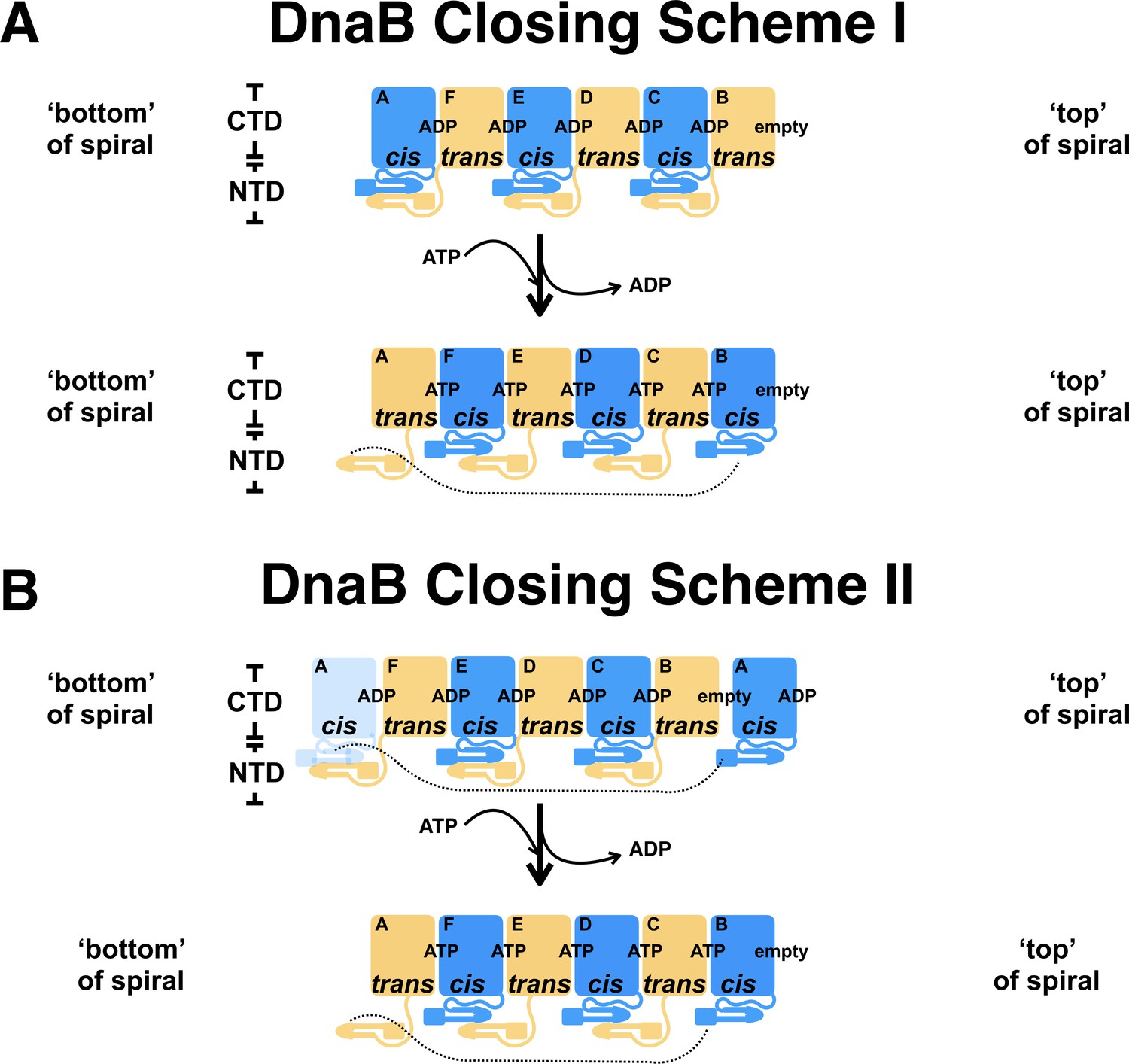
Models for closing of the DnaB helicase after expulsion of the λP helicase loader.
Comparison of the BP complex (Stage II) with the ssDNA complex (Stage IV) implies two schemes for closing of the DnaB helicase once the λP loader has been expelled from the complex. These schemes depend on how subunits in the DnaB spirals seen in Stages II/III and IV are mapped onto each other; two mapping schemes are described in the discussion and below. To visualize the two closing models, the subunits that comprise the two DnaB spirals are laid out in linear space. The CTD and NTD of DnaB and their relationships in the hexamer are depicted with simple shapes. The ‘bottom’ and ‘top’ of each spiral is indicated. Labels also indicate a chain identifier for each subunit, the nucleotide bound at subunit interfaces, and the type of DnaB isomer. Cis and trans isomers of DnaB are colored in blue and light yellow, respectively. For clarity, the λP helicase loader is not shown. (A)In closing scheme I, the CTDs of each subunit are mapped such that the positions of the ‘top’ and ‘bottom’ of each spiral correspond. The CTDs are mapped as follows: BP: chain A (cis) → ssDNA complex: chain A (trans); BP: chain B (trans)→ ssDNA complex: chain B (cis); BP: chain C (cis) → ssDNA complex: chain C (trans); BP: chain D (trans) → ssDNA complex: chain D (cis); BP: chain E (cis) → ssDNA complex: chain E (trans); BP: chain F (trans)→ ssDNA complex: chain F (cis). Since the pattern of DnaB isomers differs in the two spirals, the mapping associated with closing scheme I implies that transition from the BP (Stage II/III) to the ssDNA complex (Stage IV) will be accompanied by a cis-to-trans isomerization of DnaB subunits. Isomerization involves disruption of the dimers in the NTD tier, rotation of the dissociated NTD, followed by reformation of the dimers, but with a distinct DnaB subunit. For example, in the Stage II complex, the NTD of subunit A is bound to subunit F. However, transition to Stage IV requires swapping of dimer partners such that chain A pairs with chain B, etc. (B)Closing scheme II involves an alternate mapping of CTDs in the two DnaB spirals as follows: BP: chain A (cis) → ssDNA complex: chain B (cis); BP: chain B (trans) → ssDNA complex: chain C (trans); BP: chain C (cis) → ssDNA complex: chain D (cis); BP: chain D (trans) → ssDNA complex: chain E (trans); BP: chain E (cis) → ssDNA complex: chain F (cis); BP: chain F (trans) → ssDNA complex: chain A (trans). In this alternate mapping, closing of the DnaB helicase involves dissociation of the CTD from chain A, followed by translocation from its original position in the BP complex at the ‘bottom’ of the spiral to its new position at the ‘top’ of the spiral as indicated. Closing of the NTD tier, then, involves rotations of component NTD dimers en masse. The match between the pattern of DnaB isomers in the BP complex after translocation of the chain A CTD with that seen in the ssDNA complex implies that disruption and reformation of NTD dimers is not required. (We note that only the pattern of isomers has been matched, not the chain identifiers.) The pattern of nucleotide occupancy shown here is speculative as little is known about the nature of exchange and filling of sites during closing of the helicase. It is also clear that the same match of DnaB isomers during the transition from Stage II/III to IV could be achieved by allowing translocation of a CTD from the ‘top’ to the ‘bottom’ of the spiral; we consider this scheme to be a variant of closing scheme II.
Author response image 1
Untagged DnaB • λP does not bind nonspecifically to NiNTA beads.
https://doi.org/10.7554/eLife.41140.031Videos
Video 1
Opening the CTD layer of the DnaB-helicase by the λP helicase loader.
This movie depicts the transition of the CTD layer of the DnaB helicase from the closed planar constricted form (Stage I, PDB = 4NMN) to the right handed open spiral form (Stage II, this work). The CTDs are depicted in a ribbon representation (left) and as spheres drawn around the respective centers of mass (right). The ribbon and sphere representations are colored as in Figure 5A. The pseudo-helical axis is aligned with the vertical. In Videos 1 and 3, only the end states arise from experimentally determined coordinates; the intermediate structures were calculated by the morph algorithm (PyMOL), and, as such, may be incomplete or contain errors.
Video 2
Opening and closing of the DnaB-helicase.
This video depicts the transition of the CTD and NTD layers from the DnaB helicase from the closed planar form (Stage I, PDB = 4NMN) to the right-handed open spiral form (Stage II, this work) to the right- handed closed spiral form of Stage IV (PDB = 4ESV). The DnaB protomers are depicted in a ribbon representation (left) and as spheres drawn around the respective centers of mass of each CTD and cylinders/spheres drawn around the around the respective centers of mass of the globe domain and helical hairpin of each NTD (right). Five molecules of the λP helicase loader (depicted in a ribbon representation and colored in gray) bind to the DnaB helicase and mediate the transitions depicted in the video. ssDNA (depicted in a sticks representation and colored in red) is depicted as binding to the helicase•loader complex prior to transition to the Stage IV conformer. The DnaB protomers are colored as in Figure 5A. For Video 2, only the end and mid states arise from experimentally determined coordinates; the intermediate structures were calculated by the morph algorithm (PyMOL), and, as such, may be incomplete or contain errors.
Video 3
Opening of the NTD layer of the DnaB-helicase by the λP helicase loader.
This movie depicts transition of the NTD layer of the DnaB helicase from the closed planar constricted form (Stage I, PDB = 4NMN) to the right-handed open spiral form (Stage II, this work). The NTDs are depicted in a ribbon representation (left) and as cylinders/spheres drawn around the respective centers of mass of the globe domain and the helical hairpin of each NTD (right). The ribbon and cylinder/sphere representations are colored as in Figure 5A.
Tables
Table 1
Data collection and model refinement.
https://doi.org/10.7554/eLife.41140.013| Data collection | |
|---|---|
| Microscope/Camera | Titan Krios 300kV/Gatan K2 Summit |
| Pixel size (Å) | 1.07 |
| Defocus range (μm) | −1.0 to −3.0 |
| Cell Dimensions | |
| a, b, c (Å) | 273.92, 273.92, 273.92 |
| α, β, γ (degrees °) | 90, 90, 90 |
| Reconstruction | |
| Particles | 90,883 |
| Resolution (Å) | 4.1 |
| Model Refinement | |
| Program | Phenix (real_space_refine) |
| Resolution Limit (Å) | 4.1 |
| Number of chains | 11 |
| Number of residues | 3280 |
| RMS bond length (Å) | 0.008 Å |
| RMS bond angle (degrees º) | 1.099 |
| Ramachandran plot | |
| Preferred (%) | 84.56 |
| Allowed (%) | 15.26 |
| Outliers (%) | 0.18 |
| MolProbity | |
| Clash score | 9.87 |
| Rotamer outliers (%) | 0.58 |
Table 2
Crosslinked peptides provided by the CX-MS procedure and their interpretation in terms of the EM model.
https://doi.org/10.7554/eLife.41140.014| Peptide | Protein 1 | Residue 1 | Protein 2 | Residue 2 | Consistency with BP EM model |
|---|---|---|---|---|---|
| ALAKELNVPVVALSQLNR(4)-ANKDEGPK(3):0 | EcDnaB | 373 | EcDnaB | 175 | Yes |
| VFKIAESR(3)-ANKDEGPK(3):0 | EcDnaB | 167 | EcDnaB | 175 | Yes |
| KTAGLQPSDLIIVAAR(1)-VDQTKIR(5):0 | EcDnaB | 217 | EcDnaB | 283 | Yes |
| ISGTMGILLEKR(11)-VDQTKIR(5):0 | EcDnaB | 307 | EcDnaB | 283 | Yes |
| ALAKELNVPVVALSQLNR(4)-VFKIAESR(3):0 | EcDnaB | 373 | EcDnaB | 167 | Yes |
| ALAKELNVPVVALSQLNR(4)-AGNKPFNK(1):0 | EcDnaB | 373 | EcDnaB | 2 | DnaB residue two is not observed in our map |
| ANKDEGPKNIADVLDATVAR(8)-VFKIAESR(3):0 | EcDnaB | 180 | EcDnaB | 167 | Yes |
| ANKDEGPKNIADVLDATVAR(8)-ALAKELNVPVVALSQLNR(4):0 | EcDnaB | 180 | EcDnaB | 373 | Yes |
| KAADELVHMTAR(1)-ADKRPVNSDLR(3):0 | lambdaP | 177 | EcDnaB | 395 | Yes |
| GEAIPEPVKQLPVMGGR(9)-VDQTKIR(5):0 | lambdaP | 200 | EcDnaB | 283 | Yes |
| INRGEAIPEPVKQLPVMGGR(12)-KTAGLQPSDLIIVAAR(1):0 | lambdaP | 200 | EcDnaB | 217 | Yes |
| ANKDEGPK(3)-FGLKGASV(4):0 | EcDnaB | 175 | lambdaP | 229 | Yes |
| AGNKPFNK(1)-FGLKGASV(4):0 | EcDnaB | 2 | lambdaP | 229 | DnaB residue two is not observed in our map |
| VFKIAESR(3)-FGLKGASV(4):0 | EcDnaB | 167 | lambdaP | 229 | Yes |
| ALAKELNVPVVALSQLNR(4)-GEAIPEPVKQLPVMGGR(9):0 | EcDnaB | 373 | lambdaP | 200 | No |
| ALAKELNVPVVALSQLNR(4)-FGLKGASV(4):0 | EcDnaB | 373 | lambdaP | 229 | Yes |
| AQALAKIAEIK(6)-AKFGLK(2):0 | lambdaP | 218 | lambdaP | 225 | Yes |
| FGLKGASV(4)-IAEIKAK(5):0 | lambdaP | 229 | lambdaP | 223 | Yes |
| GEAIPEPVKQLPVMGGR(9)-KAADELVHMTAR(1):0 | lambdaP | 200 | lambdaP | 177 | Yes |
| IANNMPEQYDEKPQVQQVAQIINGVFSQLLATFPASLANR(12)-MKNIAAQMVNFDR(2):0 | lambdaP | 30 | lambdaP | 2 | Lambda P residues 2 and 30 are not observed in our map |
Table 3
Mass measurements from the native MS analysis of DnaB and λP assemblies.
https://doi.org/10.7554/eLife.41140.015| Sample condition | Measured Mass ± SD (Da)* | Assemblies | Expected mass (Da)† | ∆ mass (Da) | % Mass Error | ||
|---|---|---|---|---|---|---|---|
| BP sample in 450 mM ammonium acetate, pH 7.5, 0.5 mM magnesium acetate, 0.01% Tween-20 | |||||||
| 4,46,500 | ± | 60 | B6P5 | 4,46,145 | 355 | 0.08 | |
| 4,73,100 | ± | 50 | B6P6 | 4,72,663 | 437 | 0.09 | |
| 4,19,950 | ± | 50 | B6P4 | 4,19,627 | 324 | 0.08 | |
| BP sample + oriλP ssDNA in 450 mM ammonium acetate, pH 7.5, 0.5 mM magnesium acetate, 0.01% Tween-20 | |||||||
| 4,59,480 | ± | 15 | B6P5 + one oriλP ssDNA | 4,59,285 | 195 | 0.04 | |
| BP sample in 500 mM ammonium acetate, 0.01% Tween-20‡ | |||||||
| 4,46,270 | ± | 20 | B6P5 | 4,46,145 | 125 | 0.03 | |
| 4,72,840 | ± | 20 | B6P6 | 4,72,663 | 177 | 0.04 | |
| 4,19,750 | ± | 15 | B6P4 | 4,19,627 | 124 | 0.03 | |
-
* Calculated from the average and corresponding standard deviation of all the measured masses across the charge-state distribution (n ≥ 4). Only the peak series with signals above 10% relative intensity were processed and deconvoluted.
† The expected masses include DnaB (N-terminal Met loss), 52,259 Da; λP, 26,518 Da; Oriλ-derived ssDNA (5' and 3'-OH), 13,141 Da.
-
‡Better mass accuracies were observed for protein samples in ammonium acetate without magnesium acetate due to the absence of magnesium adduction.
Key resources table
| Reagent type (species) or resource | Designation | Source or reference | Identifiers | Additional information |
|---|---|---|---|---|
| Chemical compound, drug | Isopropyl-β-D-thiogalactoside (IPTG) | Sigma-Aldrich | 367-93-1 | |
| Chemical compound, drug | Tris(hydroxymethyl)aminomethane (Tris) | Sigma-Aldrich | 77-86-1 | |
| Chemical compound, drug | Glycerol | Fisher | 56-81-5 | |
| Chemical compound, drug | 1,4-Dithiothreitol (DTT) | Sigma-Aldrich | 3843-12-3 | |
| Chemical compound, drug | Sodium chloride | Fisher | 7647-14-5 | |
| Chemical compound, drug | Adenosine 5′-triphosphate (ATP) | Sigma-Aldrich | 34369-07-8 | |
| Chemical compound, drug | Magnesium chloride | Sigma-Aldrich | 7786-30-3 | |
| Chemical compound, drug | HEPES | Sigma-Aldrich | 75277-39-3 | |
| Chemical compound, drug | Potassium phosphate dibasic | Sigma-Aldrich | 7778-77-0 | |
| Chemical compound, drug | Potassium phosphate monobasic | Sigma-Aldrich | 7758-11-4 | |
| Chemical compound, drug | Potassium chloride | Fisher | 7747-40-7 | |
| Chemical compound, drug | 4-Morpholineethanesulfonic acid (MES) | Sigma-Aldrich | 1266615-59-1 | |
| Chemical compound, drug | DSS (disuccinimidyl suberate) | Fisher | A39267 | |
| Chemical compound, drug | Ethylenediaminetetraacetic acid (EDTA) | Sigma-Aldrich | 60-00-4 | |
| Commercial assay or kit | HiTrap Q Fast Flow | GE Healthcare Life Sciences | 17-1153-01 | |
| Commercial assay or kit | HiTrap Heparin Fast Flow | GE Healthcare Life Sciences | 17-0406-01 | |
| Commercial assay or kit | Methyl Hydrophobic Interaction Chromatography | BioRad | 156–0080 | |
| Commercial assay or kit | Superdex 200 | GE | 17-1043-01 | |
| Commercial assay or kit | Zeba microspin desalting columns | Thermo Scientific | ||
| Strain, strain background (Escherichia coli) | BL21(DE3) | Novagen | 69450–3 | |
| Strain, strain background (Escherichia coli) | Rosetta | Novagen | 70954–3 | |
| Recombinant DNA reagent | pET24a-Ecoli-DnaB | Bacterial expression vector for the E. coli DnaB helicase | N/A | |
| Recombinant DNA reagent | pCDF-LP | Bacterial expression vector for the LP helicase loader from bacteriophage lambda | N/A | |
| Recombinant DNA reagent | pET24a-AA-DnaB | Bacterial expression vector for the Aquifex aeoliucs DnaB helicase | N/A | |
| Recombinant DNA reagent | pET24a-AA-DnaC | Bacterial expression vector for the Aquifex aeoliucs DnaC helicase loader | N/A | |
| Software, algorithm | Appion | (Voss et al., 2010) | ||
| Software, algorithm | Appion-Protomo | (Noble and Stagg, 2015) | http://appion.org | |
| Software, algorithm | CCP4 | (Winn et al., 2011) | http://www.ccp4.ac.uk | |
| Software, algorithm | COOT | (Emsley et al., 2010) | https://www2.mrc-lmb.cam.ac.uk/ personal/pemsley/coot/ | |
| Software, algorithm | CTFFind4 | (Rohou and Grigorieff, 2015) | http://grigoriefflab.janelia.org/ctffind4 | |
| Software, algorithm | Cryosparc | (Punjani et al., 2017) | https://cryosparc.com | |
| Software, algorithm | Dali Server | (Holm and Rosenström, 2010) | http://ekhidna.biocenter.helsinki.fi/dali_server | |
| Software, algorithm | Dynamo | (Castaño-Díez et al., 2012) | https://wiki.dynamo.biozentrum.unibas.ch/w/index.php/Main_Page | |
| Software, algorithm | EMAN2 | (Tang et al., 2007) | http://blake.bcm.tmc.edu/EMAN2/ | |
| Software, algorithm | gAutomatch | http://www.mrc-lmb.cam.ac.uk/kzhang/Gautomatch/ | ||
| Software, algorithm | gCTF | (Zhang, 2016) | http://www.mrc-lmb.cam.ac.uk/kzhang/Gctf/ | |
| Software, algorithm | LEGINON | (Suloway et al., 2005) | http://emg.nysbc.org/redmine/projects/leginon/wiki/Leginon_Homepage | |
| Software, algorithm | LSQMan | (Kleywegt, 2007; Kleywegt and Jones, 1997) | http://xray.bmc.uu.se/usf/ | |
| Software, algorithm | MOLREP | (Vagin and Teplyakov, 2010) | http://www.ccp4.ac.uk/html/molrep.html | |
| Software, algorithm | MotionCor2 | (Li et al., 2013) | http://msg.ucsf.edu/em/software/motioncor2.html | |
| Software, algorithm | PDBeFold Server | (Krissinel and Henrick, 2004) | http://www.ebi.ac.uk/msd-srv/ssm/ | |
| Software, algorithm | PHENIX | (Adams et al., 2010) | http://www.phenix-online.org/ | |
| Software, algorithm | PyMOL | (Schrodinger LLC, 2017) | http://www.pymol.org | |
| Software, algorithm | Relion | (Scheres, 2012) | https://www2.mrc- lmb.cam.ac.uk/ relion/index.php/Main_Page | |
| Software, algorithm | ResMap | (Kucukelbir et al., 2014) | http://resmap.sourceforge.net/ | |
| Software, algorithm | SFCHECK | (Vaguine et al., 1999) | http://www.ccp4.ac.uk/html/sfcheck.html | |
| Software, algorithm | Swiss-Model | (Biasini et al., 2014) | https://swissmodel.expasy.org | |
| Software, algorithm | TOMO3D | (Agulleiro and Fernandez, 2015) | https://sites.google.com/site/3demimageprocessing/tomo3d | |
| Software, algorithm | UCSF Chimera | (Pettersen et al., 2004) | https://www.cgl.ucsf.edu/chimera/ |
Table 4
Protein purification buffers.
https://doi.org/10.7554/eLife.41140.027| Protein | Purification step | Buffer |
|---|---|---|
| BP | Cell Lysis | 50 mM Tris-HCl pH 7.6, 10% (w/v) sucrose, 500 mM NaCl, 2 mM DTT, 10 mM MgCl2 |
| BP | Q-sepharose Chromatography | Q-0: 20 mM Tris pH 7.6, 5% glycerol, 1 mM DTT, 5 mM MgCl2, 0.1 mM ATP Q-A: 20 mM Tris pH 7.6, 5% glycerol, 1 mM DTT, 5 mM MgCl2, 0.1 mM ATP, 50 mM NaCl Q-B: 20 mM Tris pH 7.6, 5% glycerol, 1 mM DTT, 5 mM MgCl2, 0.1 mM ATP, 1 M NaCl |
| BP | Heparin Chromatography | H-0: 10 mM HEPES pH 7.0, 5% glycerol, 1 mM DTT, 5 mM MgCl2, 0.1 mM ATP H-A: 10 mM HEPES pH 7.0, 5% glycerol, 1 mM DTT, 5 mM MgCl2, 0.1 mM ATP, 50 mM NaCl H-B: 10 mM HEPES pH 7.0, 5% glycerol, 1 mM DTT, 5 mM MgCl2, 0.1 mM ATP, 1 M NaCl |
| BP | Methyl Chromatography | M-A: 20 mM Tris-HCl pH 8.2, 5% glycerol, 1 mM DTT, 5 mM MgCl2, 0.1 mM ATP, 1 M (NH4)2SO4 M-B: 20 mM Tris-HCl pH 8.2, 5% glycerol, 1 mM DTT, 5 mM MgCl2, 0.1 mM ATP |
| BP | Dialysis | 20 mM Na-HEPES pH 7.5, 450 mM NaCl, 5% glycerol, 2 mM DTT, 0.5 mM MgCl2, 0.5 mM ATP |
| BC | Cell Lysis | 50 mM potassium phosphate pH 7.6, 500 mM KCl, 10% glycerol, 10 mM β-mercaptoethanol |
| BC | Heparin Sepharose Chromatography | H-0: 20 mM MES pH 6.0, 5% glycerol, 1 mM DTT H-A: 20 mM MES pH 6.0, 50 mM KCl, 5% glycerol, 1 mM DTT H-B: 20 mM MES pH 6.0, 1 M KCl, 5% glycerol, 1 mM DTT |
| BC | Q-sepharose Chromatography | Q-0: 20 mM Tris pH 8.7, 10% glycerol, 10 mM MgCl2 Q-A: 20 mM Tris pH 8.7, 10 mM KCl, 10% glycerol 10 mM MgCl2 Q-B: 20 mM Tris pH 8.7, 1 M KCl, 10% glycerol, 10 mM MgCl2 |
| BC | Size Exclusion Chromatography | 20 mM MES pH 6.0, 500 mM KCl, 10% glycerol, 1 mM DTT, 0.1 mM EDTA |
Additional files
-
Transparent reporting form
- https://doi.org/10.7554/eLife.41140.028
Download links
A two-part list of links to download the article, or parts of the article, in various formats.
Downloads (link to download the article as PDF)
Open citations (links to open the citations from this article in various online reference manager services)
Cite this article (links to download the citations from this article in formats compatible with various reference manager tools)
Mechanisms of opening and closing of the bacterial replicative helicase
eLife 7:e41140.
https://doi.org/10.7554/eLife.41140


