Visualization of currents in neural models with similar behavior and different conductance densities
- Brandeis University, United States
Figures
Figure 1
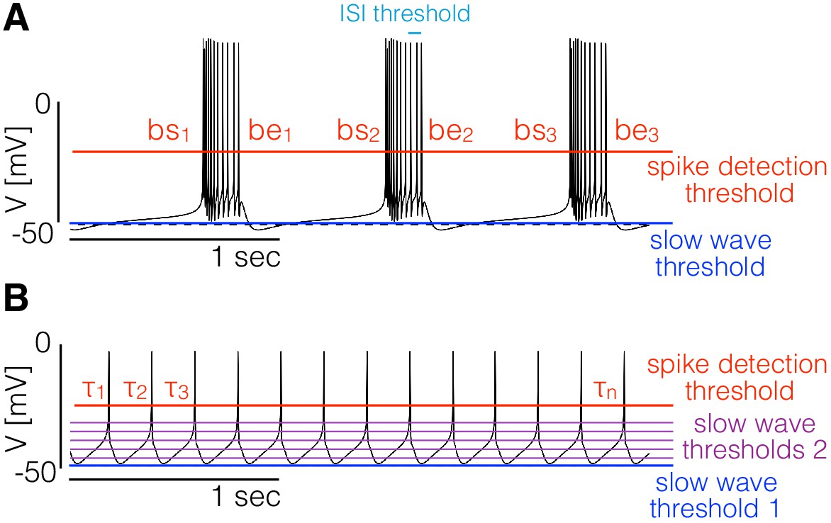
Landscape optimization can be used to find models with specific sets of features.
(A) Example model bursting neuron. The activity is described by the burst frequency and the burst duration in units of the period (duty cycle). The spikes detection threshold (red line) is used to determine the spike times. The ISI threshold (cyan) is used to determine which spikes are bursts starts (bs) and bursts ends (be). The slow wave threshold (blue line) is used to ensure that slow wave activity is separated from spiking activity. (B) Example model spiking neuron. We use thresholds as before to measure the frequency and the duty cycle of the cell. The additional slow wave thresholds (purple) are used to control the waveform during spike repolarization.
Figure 2
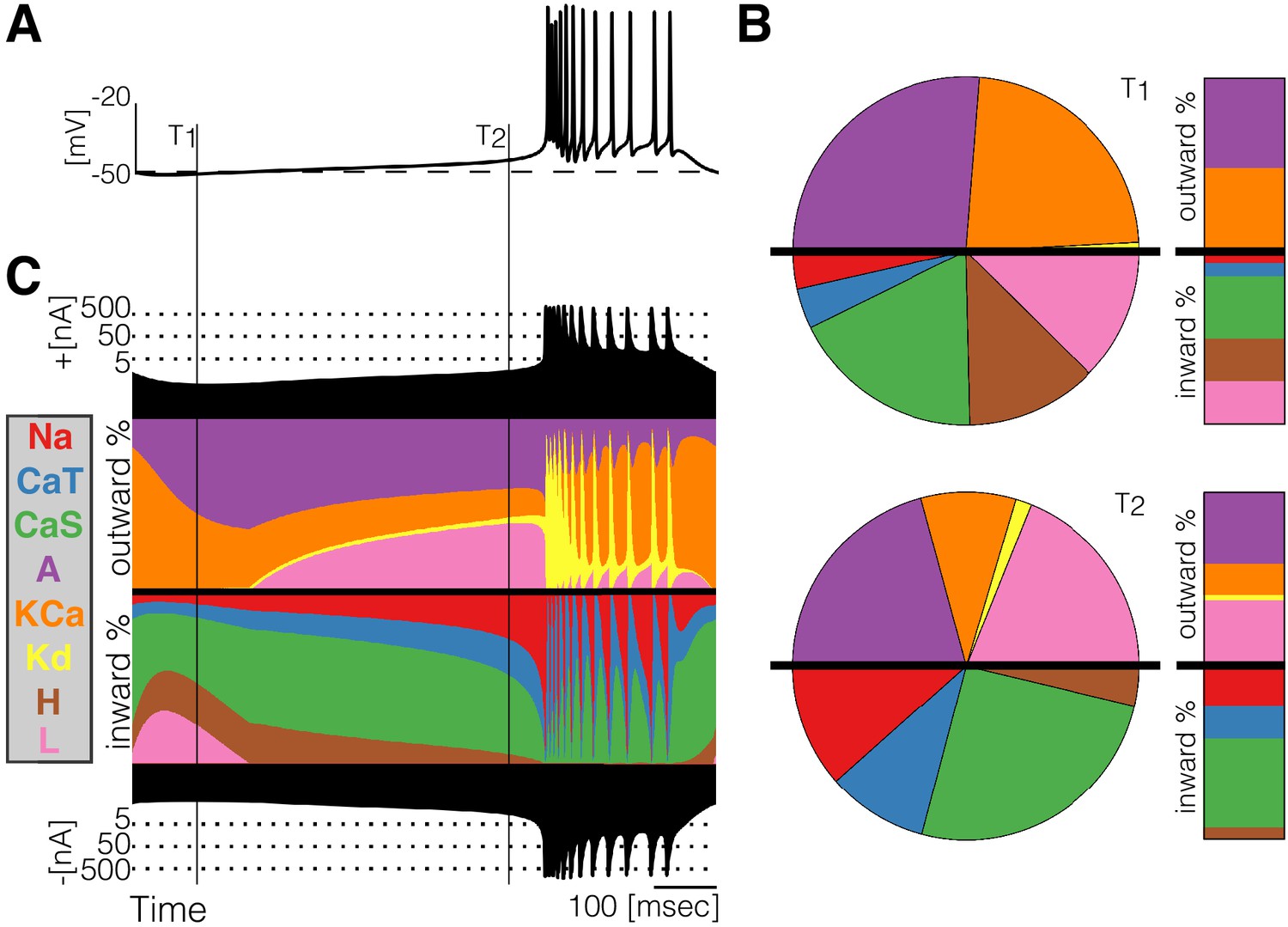
Currentscape of a model bursting neuron.
A simple visualization of the dynamics of ionic currents in conductance-based model neurons. (A) Membrane potential of a periodic burster. (B) Percent contribution of each current type to the total inward and outward currents displayed as pie charts and bars at times and (C) Percent contribution of each current to the total outward and inward currents at each time stamp. The black filled curves on the top and bottom indicate total inward outward currents respectively on a logarithmic scale. The color curves show the time evolution of each current as a percentage of the total current at that time. For example, at the total outward current is and the orange shows a large contribution of . At the total outward current has increased to and the current is contributing less to the total.
Figure 3 with 1 supplement
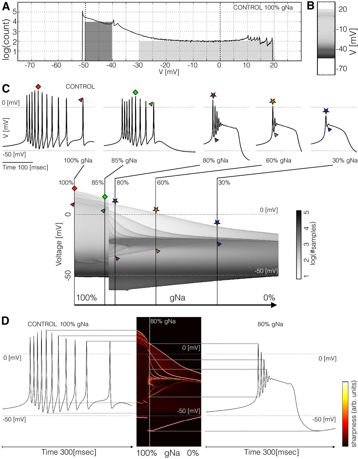
Membrane potential distributions.
(A) Distribution of membrane potential values. The total number of samples is . Y-axis scale is logarithmic. The area of the dark shaded region can be used to estimate of the probability that the activity is sampled between and , and the area of the light shaded region is proportional to the probability that is sampled between and . The area of the dark region is times larger than the light region. (B) The same distribution in (A) represented as a graded bar. (C) Distribution of as a function of and , and waveforms for several values.The symbols indicate features of the waveforms and their correspondence to the ridges of the distribution of . (D) Waveforms under two conditions and their correspondence to the ridges of the distribution of . The ridges were enhanced by computing the derivative of the distribution along the direction.
Figure 3—figure supplement 1
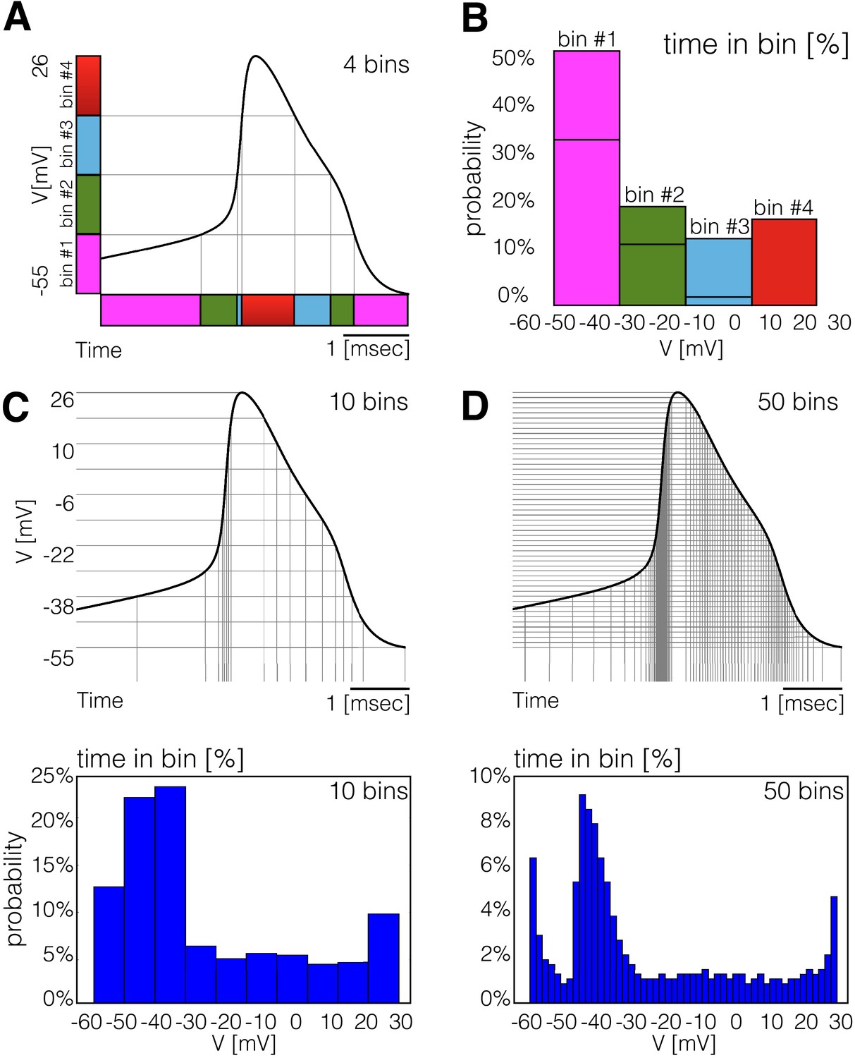
Probability distributions of membrane potential.
(A) The black trace corresponds to the membrane potential during a spike within a burst (total time ). The y-axis is split into four equally sized bins (in colors) that span the full range of V values ( and ). The probability that is observed in a given bin at a random instant is proportional to the total time spends at that bin. This is indicated in colors by the preimage of each bin. (B) The total time spent in each bin can be interpreted as a coarse-grained probability distribution of . (C) (top) Membrane potential , more bins and their pre-images. (bottom) Probability distribution of . (D) Idem for bins. Note that the probability distribution of displays sharp peaks for values of where local maxima (or minima) in time occur. This effect is more noticeable as the number of bins is increased.
Figure 4
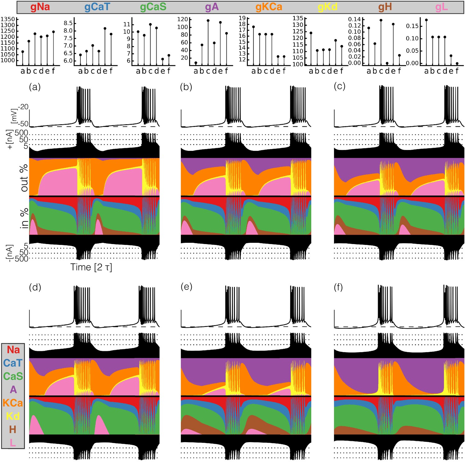
Currentscapes of model bursting neurons.
(top) Maximal conductances of all model bursters. (bottom) The panels show the membrane potential of the cell and the percent contribution of each current over two cycles.
Figure 5
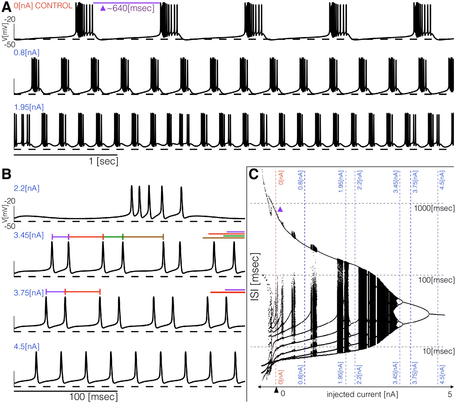
Response to current injections and interspike-intervals (ISI) distributions of model (a).
(A) (top) Control traces (no current injected ), regular bursting (), irregular bursting . (B) (top) Fast regular bursting (), quadruplets (), doublets () and singlets () (tonic spiking). (C) ISI distributions over a range of injected current.
Figure 6

ISI distributions of the six model bursting neurons over a range of injected current.
The panels show all ISI values of each model burster over a range on injected currents (vertical axis is logarithmic). All bursters transition into tonic spiking regimes for injected currents larger than and the details of the transitions are different across models.
Figure 7
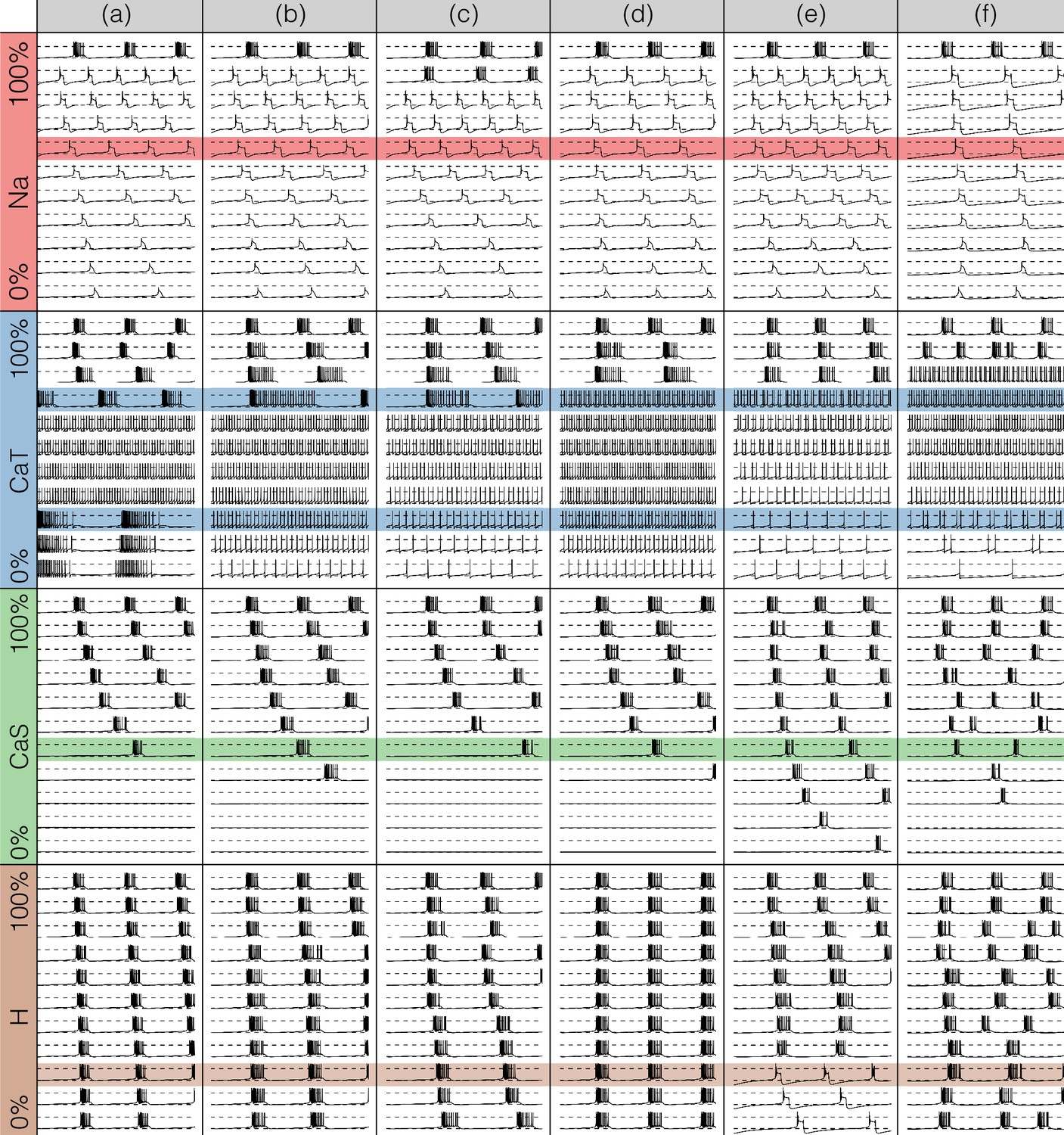
Effects of decreasing maximal conductances: inward currents.
The figure shows the membrane potential of all model cells as the maximal conductance of each current is gradually decreased from to . Each panel shows traces with a duration of 3 s. Dashed lines are placed at and . The shading indicates values of maximal conductance for which the activity the models differs the most.
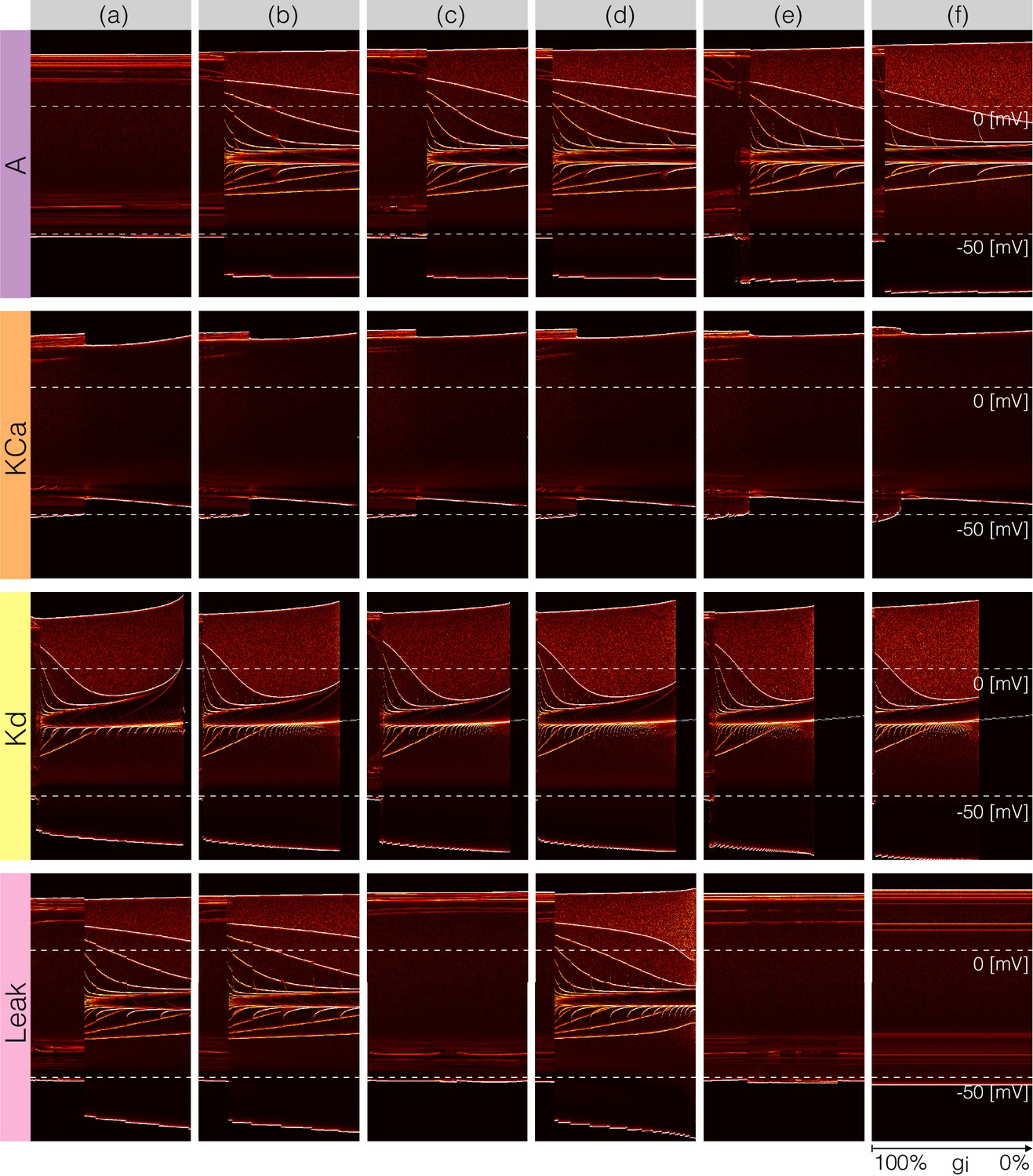
Figure 8
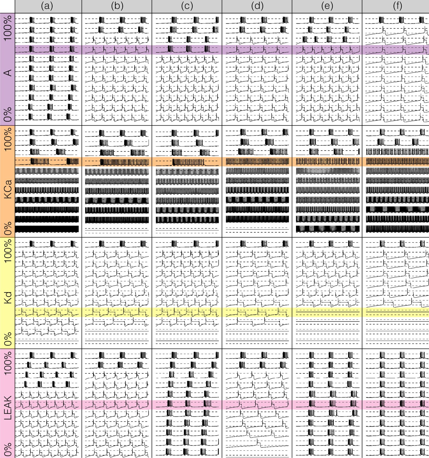
Effects of decreasing maximal conductances: outward currents.
The figure shows the membrane potential of all model cells as the maximal conductance of each current is gradually decreased from to . Each panel shows traces with a duration of 3 s. Dashed lines are placed at and . The shading indicates values of maximal conductance for which the activity the models differs the most.
Figure 9
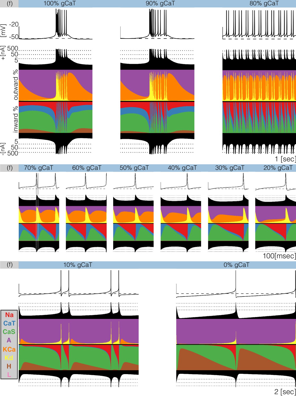
Decreasing in model (f).
The figure shows the traces and the currentscapes of model (f) as is gradually decreased. Top panels show second of data, center panels show seconds and the bottom panels show seconds (see full traces in Figure 8).
Figure 10
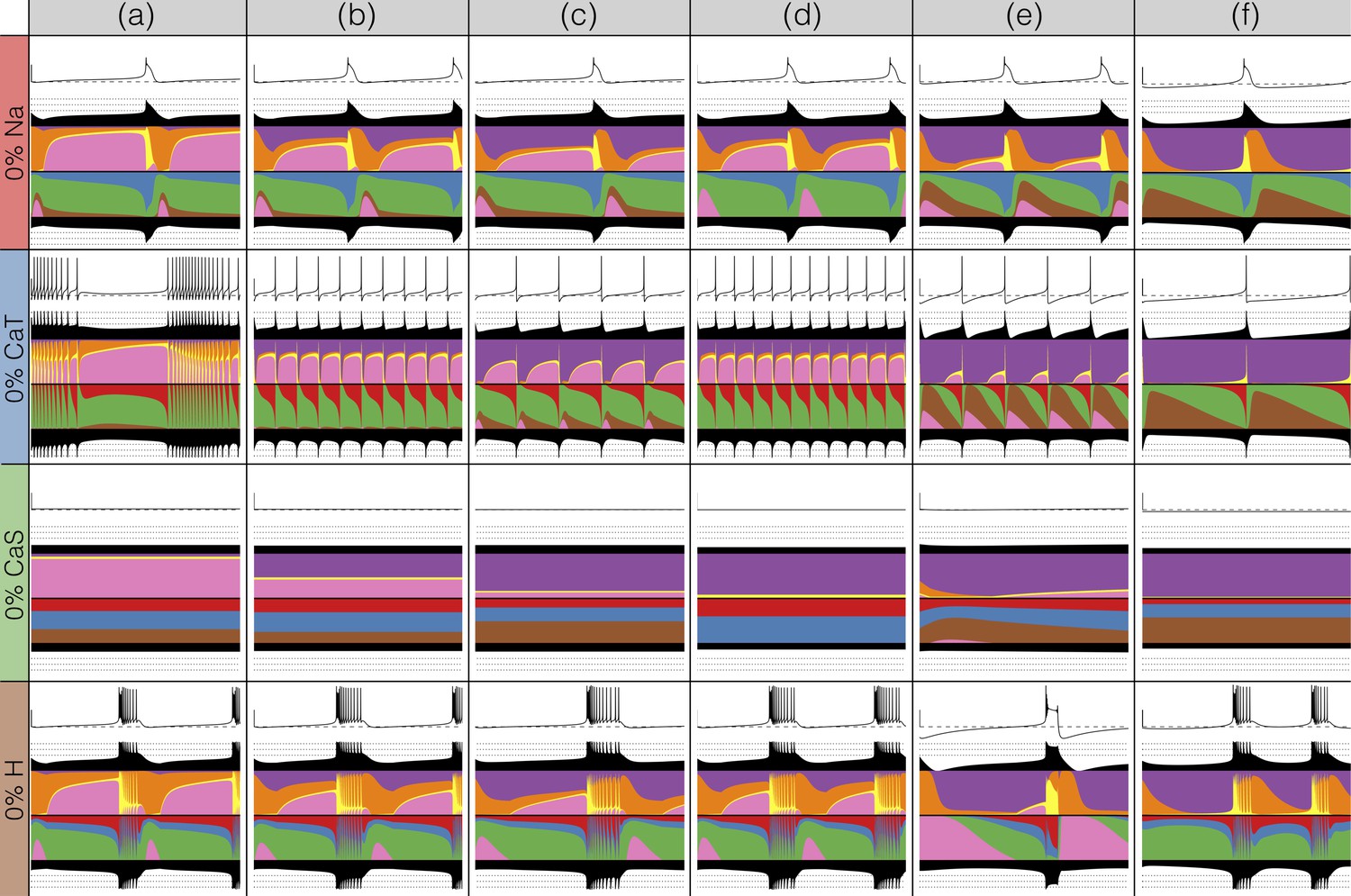
Complete removal of one current: inward currents.
The figure shows the traces and currentscapes for all bursters when one current is completely removed.
Figure 11
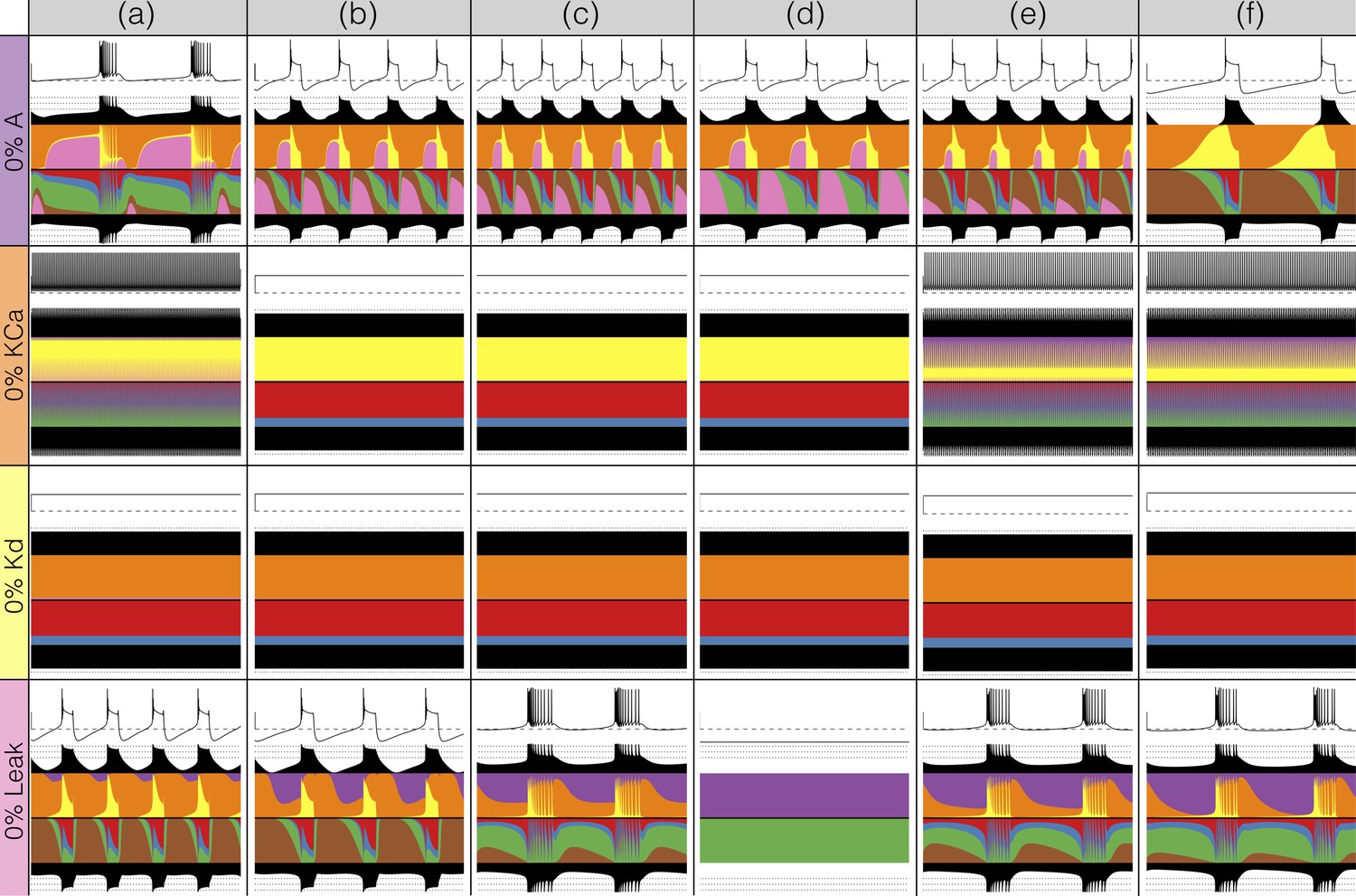
Complete removal of one current: outward currents.
The figure shows the traces and currentscapes for all bursters when one current is completely removed.
Figure 12
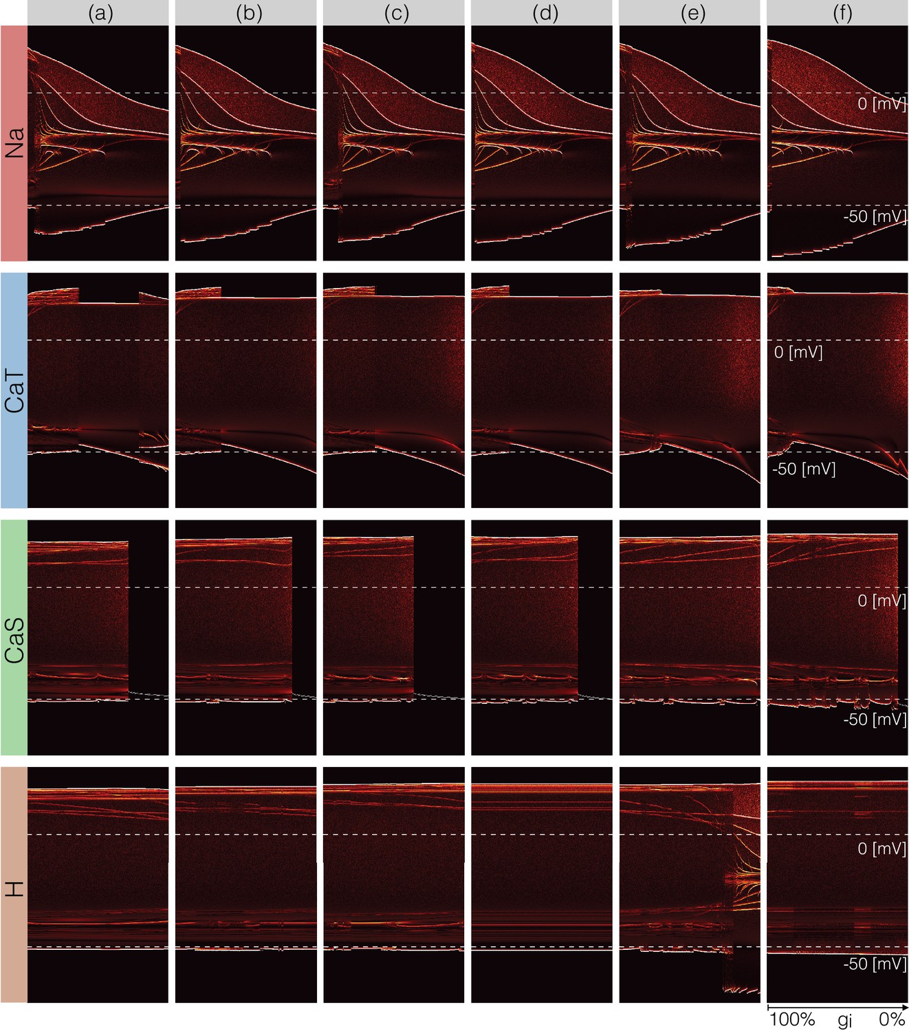
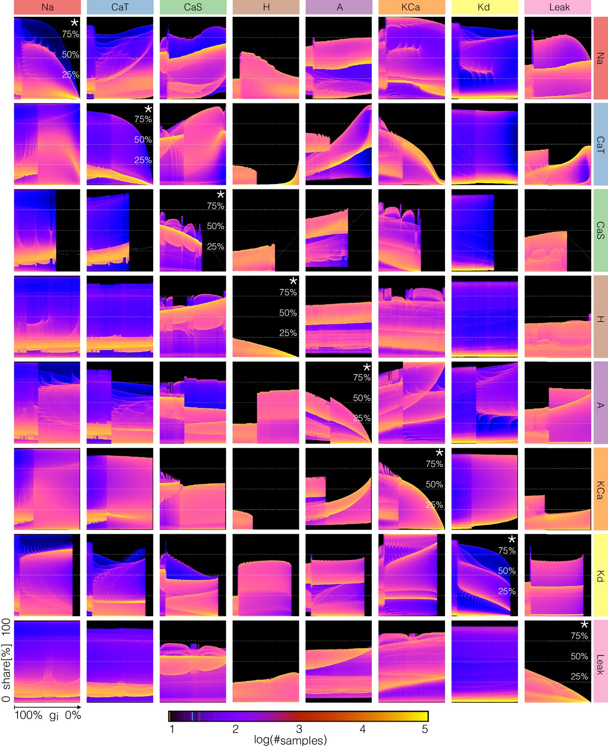
Changes in waveform as currents are gradually removed.
Inward currents. The figure shows the ridges of the probability distribution of as a function of and each maximal conductance . The ridges of the probability distributions appear as curves and correspond to values of where the system spends more time, such as extrema. The panels show how different features of the waveform such as total amplitude, and the amplitude of each spike, change as each current is gradually decreased.
Figure 13
Changes in waveform as currents are gradually removed.
Outward and leak currents. The figure shows the ridges of the probability distribution of as a function of and each maximal conductance . See Figure 12.
Figure 14 with 1 supplement
Changes in waveform of current shares as one current is gradually decreased.
The panels show the probability distribution of the share of each current for model (f) as is decreased (see Figure 14—figure supplement 1).
Figure 14—figure supplement 1
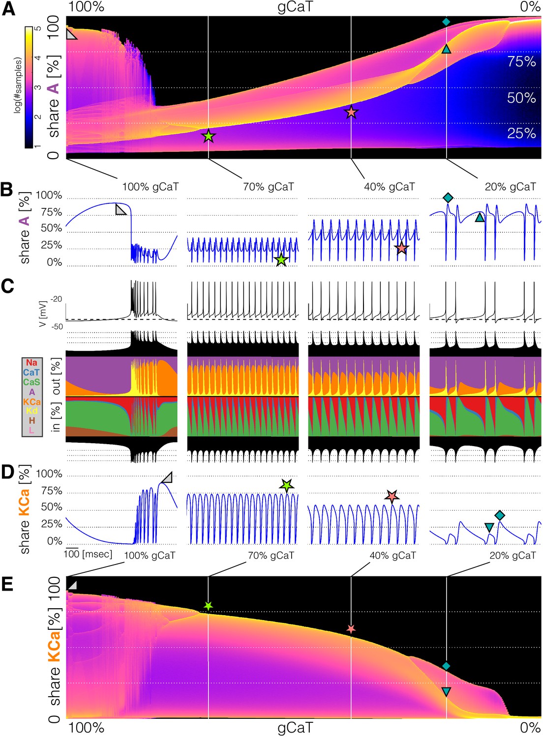
Probability distributions of currents shares.
The Figure shows the relationship between the currentscapes and the distributions of current shares. (A) Distribution of current share to the total outward current for values of between and . (B) Share of current as a time series. The current contributes with more than of the outward current for most of the time. At the cell spikes tonically and the contributes of the outward current most of the time. The symbols indicate features in the waveform that are mapped to ridges in the distribution. (C) Currentscapes. (D) Idem (B) but for . Notice the share of decreasing as . (E) Distribution of current share to the total outward current for values of between and .
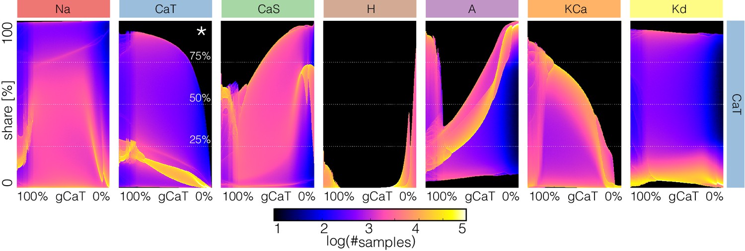
Figure 15
Changes in waveform of current shares as each current is gradually decreased.
The panels show the probability distribution of the share of each current for model (c) as each current is decreased.
Tables
Table 1
Parameters used in this study and error value.
https://doi.org/10.7554/eLife.42722.020| gNa | gCaT | gCaS | gA | gKCa | gKd | gH | gL | |||
|---|---|---|---|---|---|---|---|---|---|---|
| model (a) | 1076.392 | 6.4056 | 10.048 | 8.0384 | 17.584 | 124.0928 | 0.11304 | 0.17584 | 653.5 | 0.051 |
| model (b) | 1165.568 | 6.6568 | 9.5456 | 54.5104 | 16.328 | 110.7792 | 0.0628 | 0.10676 | 813.88 | 0.053 |
| model (c) | 1228.368 | 7.0336 | 11.0528 | 117.5616 | 16.328 | 111.2816 | 0.13816 | 0.10676 | 605.98 | 0.027 |
| model (d) | 1203.248 | 6.6568 | 10.5504 | 59.5344 | 16.328 | 111.4072 | 0.0 | 0.10676 | 653.5 | 0.471 |
| model (e) | 1210.784 | 8.164 | 6.28 | 113.04 | 12.56 | 118.4408 | 0.1256 | 0.0314 | 393.13 | 0.109 |
| model (f) | 1245.952 | 7.7872 | 6.7824 | 84.6544 | 12.56 | 113.9192 | 0.02512 | 0.0 | 174.34 | 0.047 |
| model (Figure 2) | 1228.368 | 7.0336 | 11.0528 | 117.5616 | 16.328 | 110.7792 | 0.13816 | 0.10048 | 605.98 | 0.007 |
| model (Figure 3) | 895.528 | 3.8936 | 16.5792 | 116.4312 | 21.352 | 115.6776 | 0.0 | 0.08792 | 828.73 | 0.058 |
Additional files
-
Transparent reporting form
- https://doi.org/10.7554/eLife.42722.021
Download links
A two-part list of links to download the article, or parts of the article, in various formats.
Downloads (link to download the article as PDF)
Open citations (links to open the citations from this article in various online reference manager services)
Cite this article (links to download the citations from this article in formats compatible with various reference manager tools)
Visualization of currents in neural models with similar behavior and different conductance densities
eLife 8:e42722.
https://doi.org/10.7554/eLife.42722


