Multivariate stochastic volatility modeling of neural data
- University of Pennsylvania, United States
Figures
Figure 1
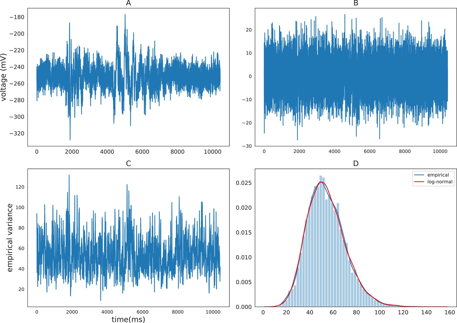
Empirical characteristics of iEEG.
(A) Sample raw iEEG time series during a resting state (count down non-task) period for subject R1240T. (B) Detrended iEEG timeseries after removing autoregressive components. (C) Empirical variance timeseries calculated using a rolling-window of size 20. (D) Distribution of empirical variance with the blue curve showing the estimated empirical density using kernel density estimation and the red curve showing the best-fitting log-normal density to the data.
Figure 2
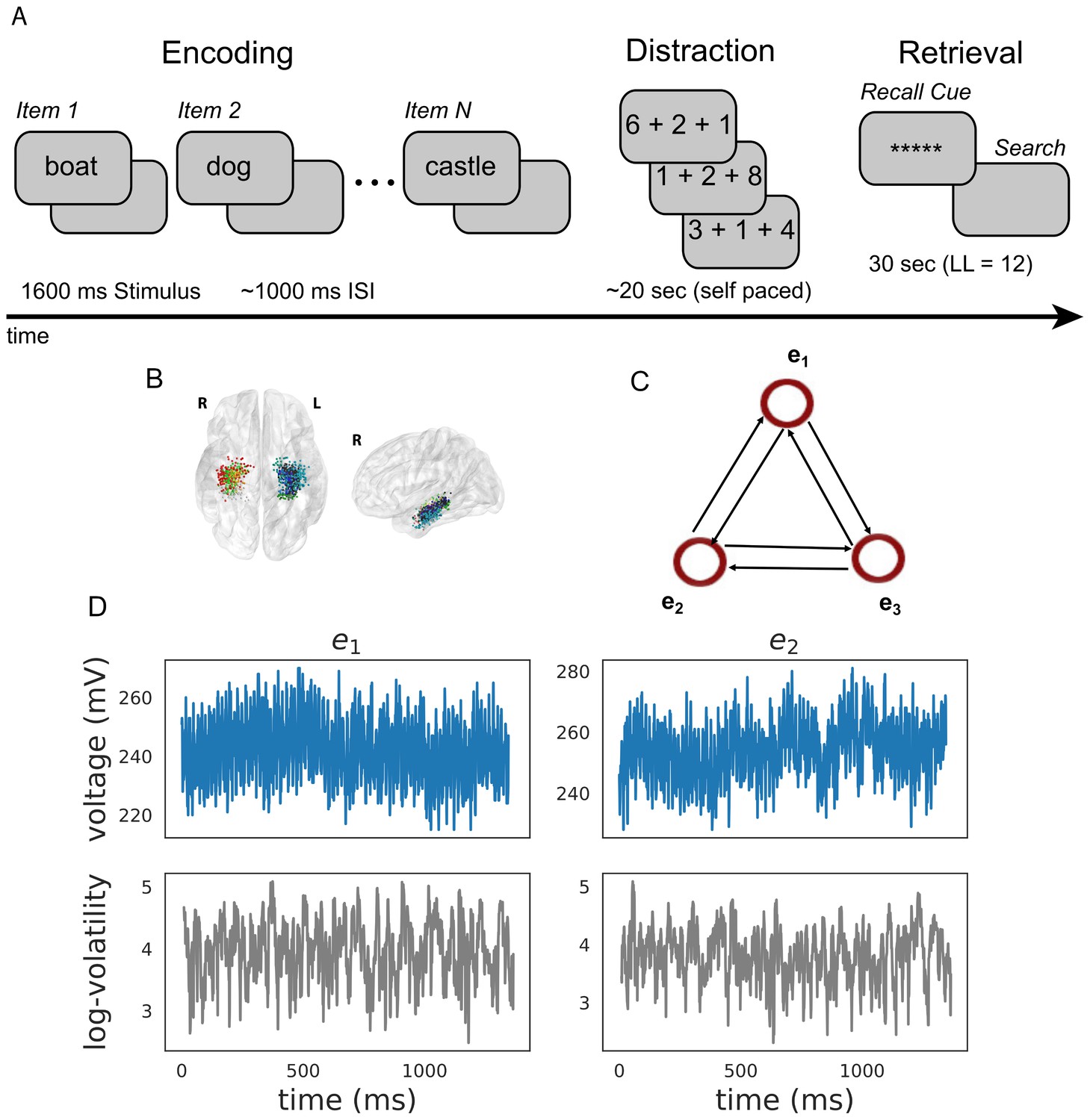
Task design and analysis.
(A) Subjects performed a verbal free-recall task which consists of three phases: (1) word encoding, (2) math distraction, and (3) retrieval. (B) 96 Participants were implanted with depth electrodes in the medial temporal lobe (MTL) with localized subregions: CA1, CA3, dentate gyrus (DG), subiculum (Sub), perirhinal cortex (PRC), entorhinal cortex (EC), or parahippocampal cortex (PHC). (C) To construct a directional connectivity network, we applied the MSV model to brain signals recorded from electrodes in the MTL during encoding. We analyzed the 1.6 s epochs during which words were presented on the screen. The network reflects directional lag-one correlations among the implied volatility timeseries recorded at various MTL subregions. (D) The upper row shows a sample of an individual patient’s raw voltage timeseries (blue) recorded from two electrodes during a word encoding period of 1.6 s, and the lower row shows their corresponding implied volatility timseries (gray) estimated using the MSV model.
Figure 3
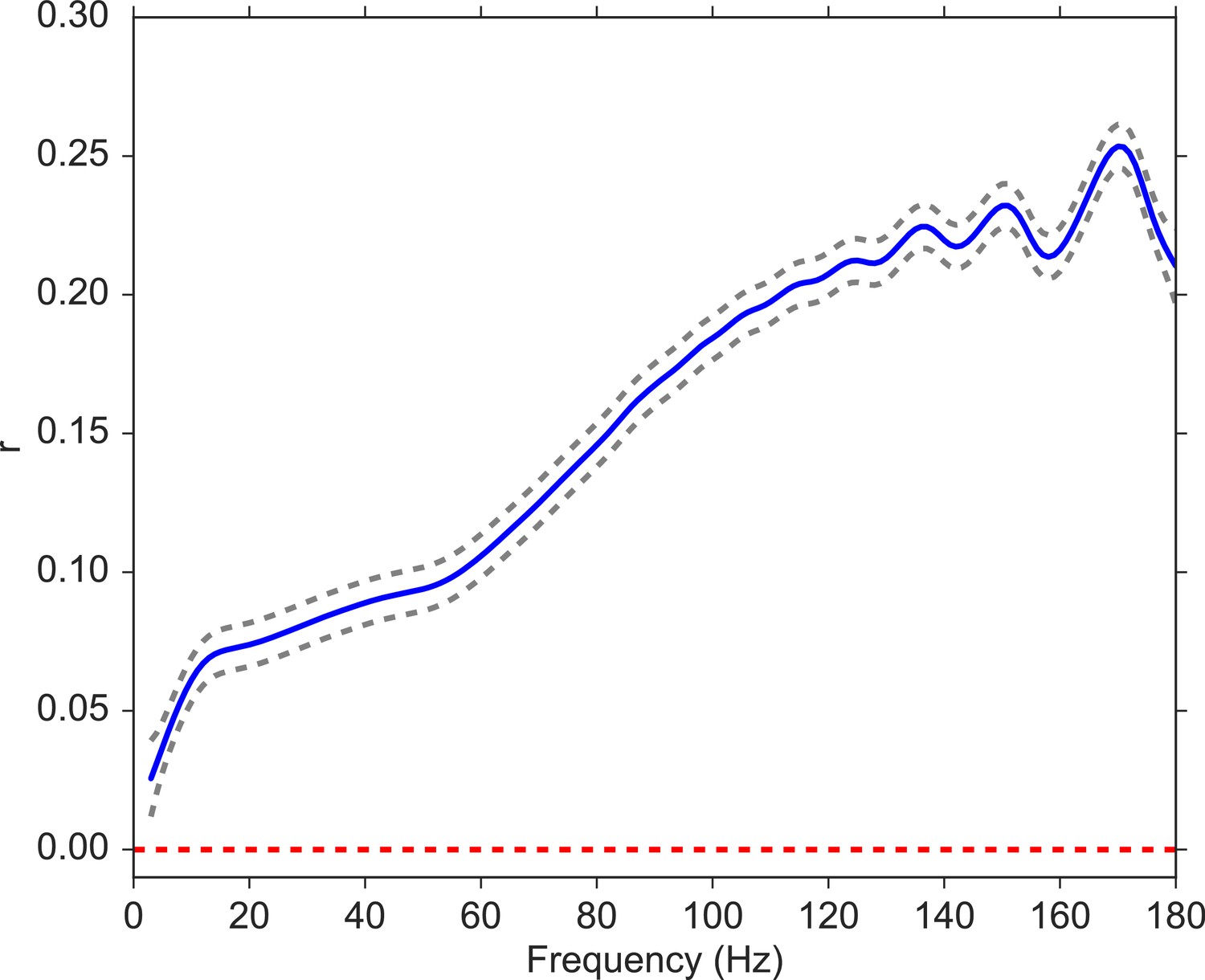
Correlation between volatility and spectral power over a frequency range from 3 to 180 Hz.
We fit a Gaussian process model to estimate the functional form of the correlation function between volatility and spectral power (solid blue line). The 95% confidence bands were constructed from 96 subjects (dashed gray lines). The red line shows the null model. We observe a significantly positive correlation between volatility and spectral power, and the correlation increases with frequency.
Figure 4
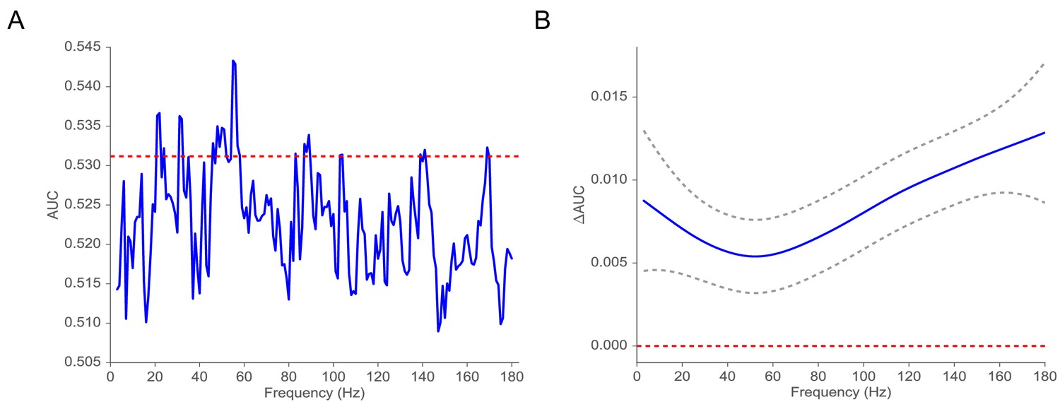
Classification of subsequent memory recall.
(A) Average AUC of the classifier trained on spectral power across 42 subjects with at least three sessions of recording (blue). The red line indicates the average AUC of the classifier trained on volatility. (B) AUC = AUCAUC as a function of frequency estimated by using a Gaussian regression model (dashed gray lines indicate 95% confidence bands). The red line shows the null model. We observe that the classifier trained on volatility performs at least as well as the one trained on spectral power across the frequency spectrum. We find that functional form of AUC is significantly different from the function (, P < ) using a Gaussian process model, suggesting that the difference in performance between the volatility classifier and the spectral power classifier is significant.
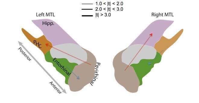
Figure 5
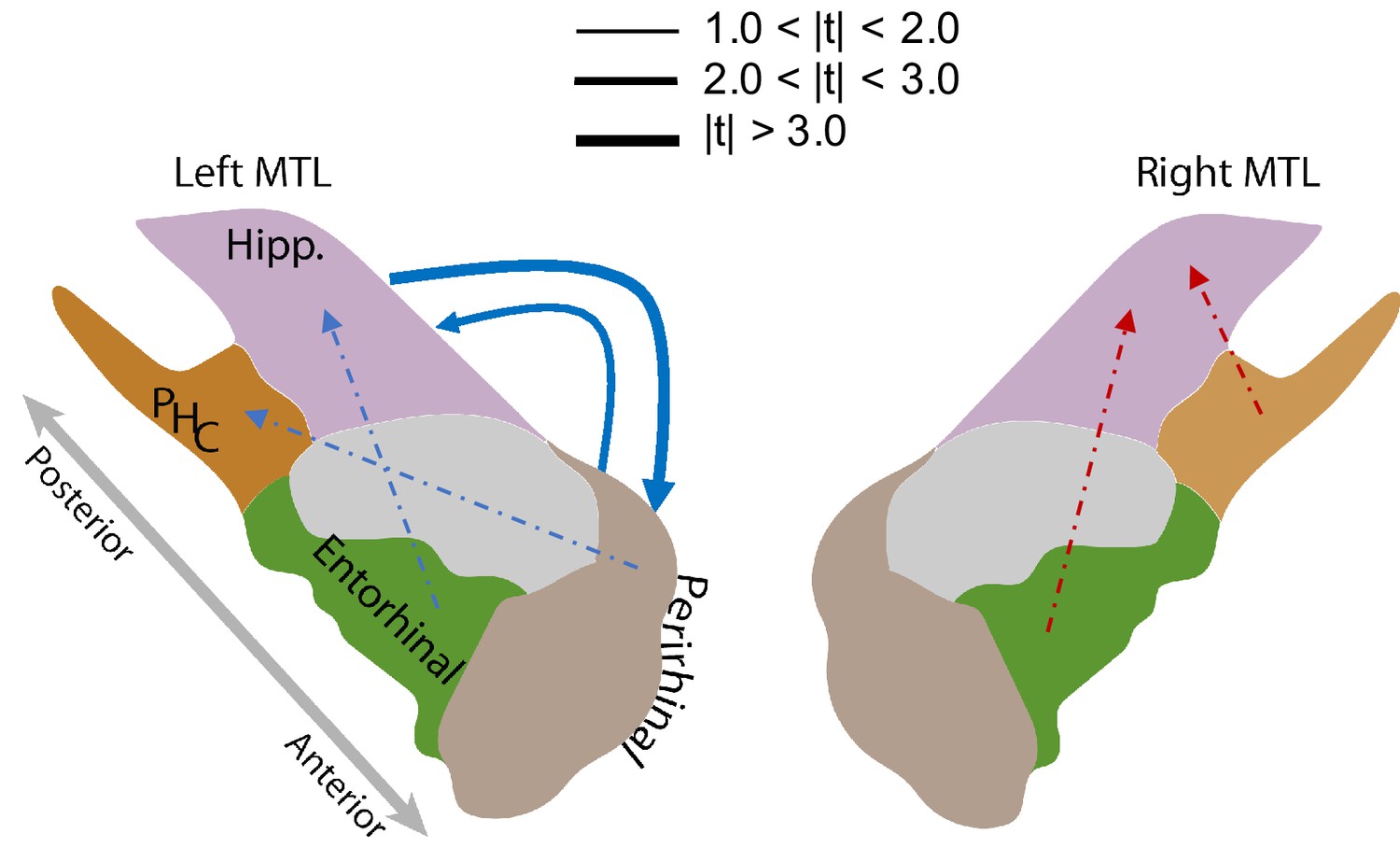
MTL directional connectivity network.
The MTL electrodes were divided into four subregions: hippocampus (Hipp.), parahippocampal cortex (PHC), entorhinal cortex (EC), and perirhinal cortex (PRC). The directional connectivity from region I to region J, , was calculated by averaging the entries of the sub-matrix of the regression coefficient matrix , whose rows and columns correspond to region I and J respectively. We computed the contrast between the directional connectivity of recalled and non-recalled events: for each subject. Solid lines show significant (FDR-corrected) connections between two regions and dashed lines show trending but insignificant connections. Red indicates positive changes and blue indicates negative changes. The directional connectivity from Hipp. to PRC is significant (adj. P < 0.01) and the reverse directional connectivity is also significant (adj. P < 0.05).
Appendix 3—figure 1

Time length analysis.
For ranging from 30 to 180 with 30 increments and for each , we simulated 30 datasets according to the data-generating process specified by the MSV model. Then, we estimated the connectivity matrix for each dataset. We assess the performance of the MSV model in estimating the true connectivity matrix using the log-determinant error metric, . The figure shows the average performance at each time length with the standard error bars.
Appendix 3—figure 2
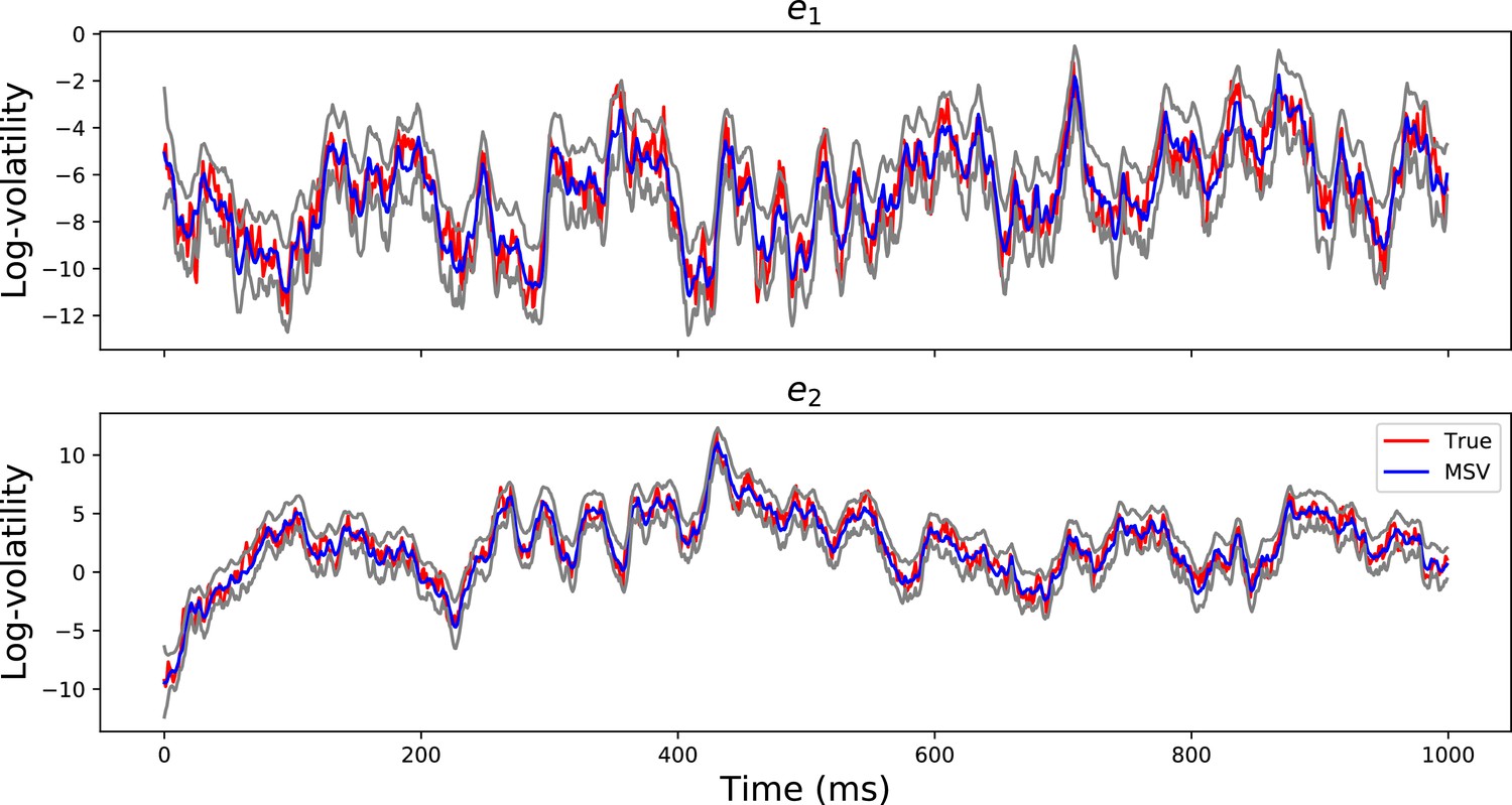
Volatility Timeseries Recovery.
The red lines show the true simulated log-volatility timeseries for the first 1000 time points for two channels . The blue timeseries show the estimated log-volatility time series using the MSV model and the gray timeseries are the 95% posterior confidence intervals. The figure demonstrates that the MSV model can estimate the latent log-volatility timeseries well.
Appendix 4—figure 1
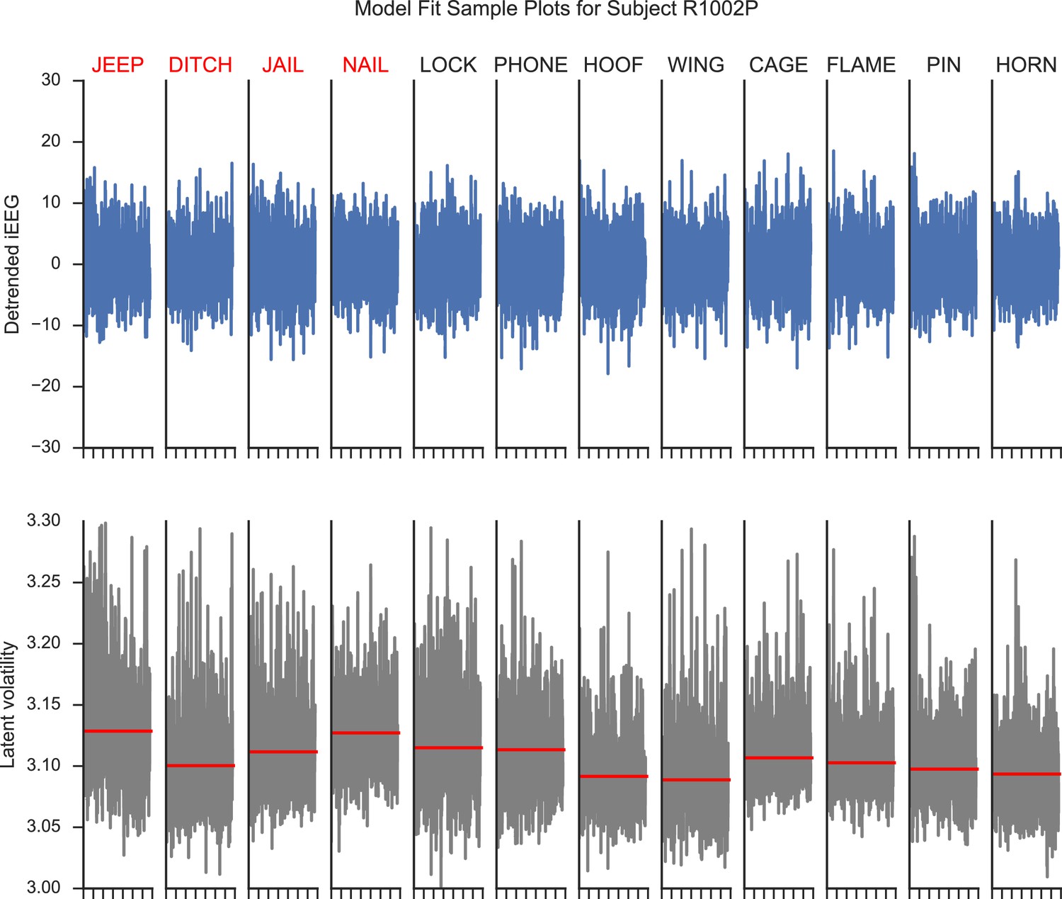
Model fit plots for a hippocampal electrode.
The upper panels show the detrended iEEG signals using an AR(p) model for encoding periods of a list of words. The lower panels show the associated estimated latent volatility processes. The red lines indicate the average volatility during the encoding period. Red words are later recalled and blue words are not recalled.
Appendix 6—figure 1

Cross-validation scheme.
For each subject, we train our classifier on all (yellow) but one session and test the performance on the hold-out session (green) and repeat the procedure for each session.
Appendix 6—figure 2
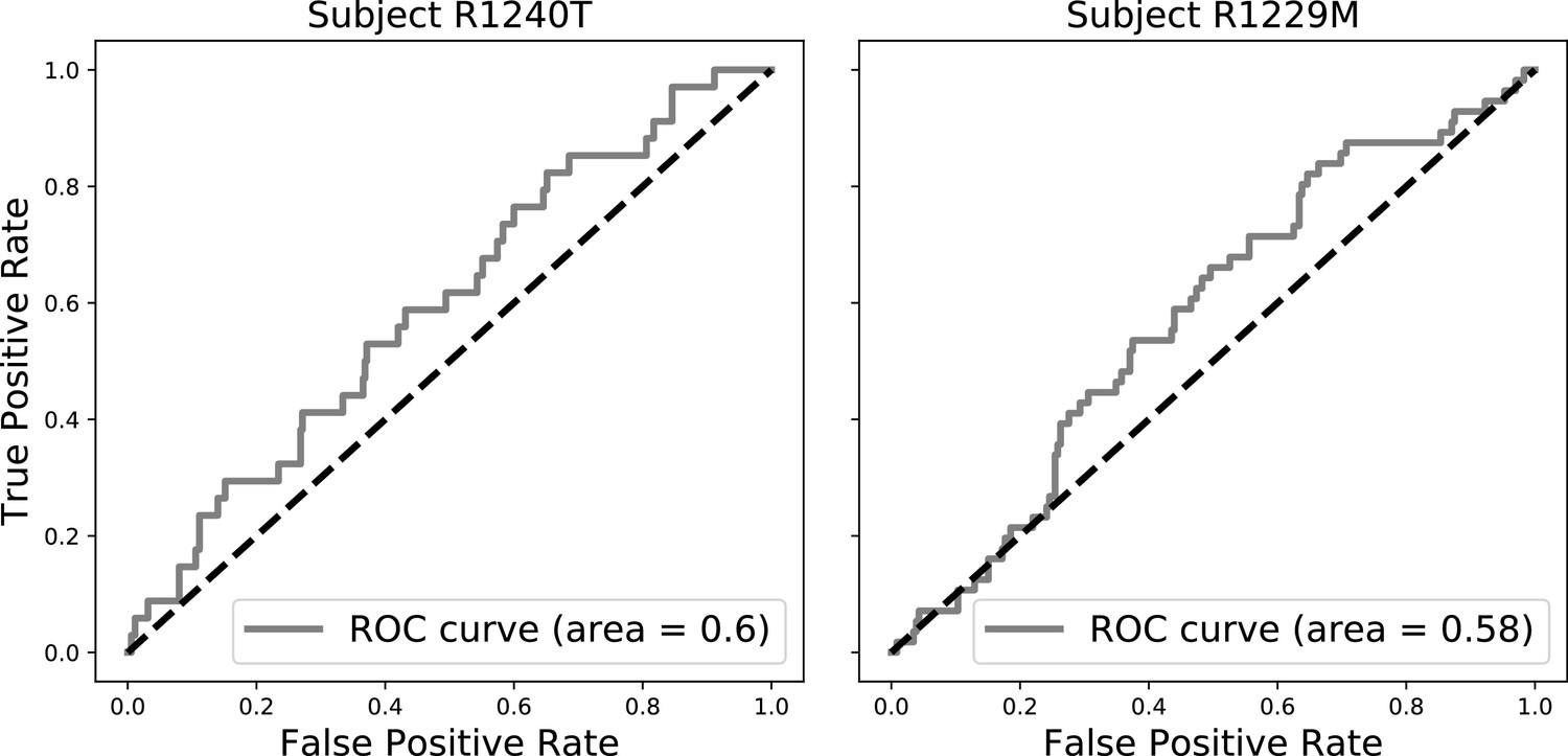
Sample ROC curves (gray).
The black dashed lines indicate ROC curves of at-chance classifiers. The area under the ROC curve (AUC) is a measure of the performance of the classifier across a spectrum of decision thresholds. An AUC of 1 indicates that the classifier can classify recalled items perfectly. An AUC of 0.5 indicates that the classifier is at chance, that is as good as a random coin flip.
Author response image 1
Resting state vs.Encoding Connectivity Contrast.
https://doi.org/10.7554/eLife.42950.024Tables
Key resources table
| Reagent, type (species) or resource | Designation | Source or reference | Identifiers | Additional Information |
|---|---|---|---|---|
| Software and algorithm | Avants et al., 2008 | http://picsl.upenn.edu/software/ants | advanced normalization tool | |
| Software and algorithm | Yushkevich et al., 2015 | https://www.nitrc.org/projects/ashs | ashs | |
| Software and algorithm | sklearnc | Pedregosa et al., 2011 | https://scikit-learn.org/stable/ | |
| Software and algorithm | This paper | http://memory.psych.upenn.edu/Electrophysiological_Data | custom processing scripts | |
| Software and algorithm | PTSA | This paper | https://github.com/pennmem/ptsa_new | processing pipeline for reading in iEEG |
Appendix 2—table 1
Parameter Recovery.
https://doi.org/10.7554/eLife.42950.010| Truth | MSV | |||||||||||||||
|---|---|---|---|---|---|---|---|---|---|---|---|---|---|---|---|---|
| Dataset | SNR | Channel | ||||||||||||||
| 1 | 0.16 | 1 | 3.39 | 0.85 | 0.20 | 0.00 | 0.00 | 0.00 | 0.17 | 3.39 | 0.86 | 0.19 | 0.00 | −0.04 | 0.00 | 0.17 |
| 2 | 3.60 | 0.00 | 0.88 | −0.10 | 0.00 | 0.00 | 0.19 | 3.60 | 0.00 | 0.87 | −0.10 | −0.00 | −0.01 | 0.19 | ||
| 3 | 3.55 | 0.00 | 0.00 | 0.87 | 0.30 | 0.00 | 0.19 | 3.53 | −0.00 | −0.00 | 0.85 | 0.29 | 0.01 | 0.20 | ||
| 4 | 3.51 | 0.00 | 0.00 | 0.00 | 0.71 | 0.00 | 0.12 | 3.51 | 0.01 | −0.00 | 0.01 | 0.69 | −0.03 | 0.14 | ||
| 5 | 3.38 | 0.00 | 0.00 | 0.00 | 0.00 | 0.80 | 0.15 | 3.38 | 0.00 | −0.01 | −0.01 | 0.06 | 0.79 | 0.15 | ||
| 2 | 0.27 | 1 | 3.60 | 0.95 | 0.20 | 0.00 | 0.00 | 0.00 | 0.21 | 3.93 | 0.95 | 0.19 | −0.00 | 0.00 | 0.00 | 0.24 |
| 2 | 3.74 | 0.00 | 0.90 | −0.10 | 0.00 | 0.00 | 0.25 | 3.82 | −0.00 | 0.90 | −0.10 | 0.00 | −0.00 | 0.25 | ||
| 3 | 3.89 | 0.00 | 0.00 | 0.93 | 0.30 | 0.00 | 0.29 | 3.81 | −0.00 | 0.00 | 0.93 | 0.30 | 0.00 | 0.29 | ||
| 4 | 3.05 | 0.00 | 0.00 | 0.00 | 0.91 | 0.00 | 0.28 | 3.04 | −0.00 | 0.01 | 0.01 | 0.91 | 0.00 | 0.28 | ||
| 5 | 3.96 | 0.00 | 0.00 | 0.00 | 0.00 | 0.95 | 0.22 | 3.97 | −0.00 | 0.00 | 0.00 | −0.00 | 0.94 | 0.22 | ||
| 3 | 0.42 | 1 | 3.25 | 0.52 | 0.20 | 0.00 | 0.00 | 0.00 | 0.42 | 3.25 | 0.51 | 0.20 | 0.01 | −0.02 | 0.01 | 0.43 |
| 2 | 3.64 | 0.00 | 0.57 | −0.10 | 0.00 | 0.00 | 0.46 | 3.63 | 0.01 | 0.55 | −0.14 | 0.02 | 0.02 | 0.46 | ||
| 3 | 3.18 | 0.00 | 0.00 | 0.58 | 0.30 | 0.00 | 0.31 | 3.18 | 0.03 | 0.01 | 0.56 | 0.32 | 0.03 | 0.31 | ||
| 4 | 3.44 | 0.00 | 0.00 | 0.00 | 0.65 | 0.00 | 0.41 | 3.45 | 0.00 | −0.00 | −0.00 | 0.64 | 0.00 | 0.41 | ||
| 5 | 3.26 | 0.00 | 0.00 | 0.00 | 0.00 | 0.60 | 0.36 | 3.26 | −0.02 | −0.00 | 0.00 | −0.01 | 0.60 | 0.36 | ||
-
We generated three datasets with different signal-to-noise ratios. The observed multivariate time-series was simulated according to the data-generating process specified by the MSV model with pre-specified parameters (truth). We then applied the MSV model to the simulated series to recover the parameters of the MSV model. In this simulation study, the non-zero off-diagonal entries of the matrix were fixed across datasets. The diagonal elements of were generated from a uniform distribution on , , and respectively. The volatilities of volatility of the electrodes were generated from a uniform distribution on , , and respectively.
Appendix 7—table 1
intra-MTL directional connectivity in the left hemisphere.
https://doi.org/10.7554/eLife.42950.021| Region I region J | Mean | Se | T | N | P | adj. P |
|---|---|---|---|---|---|---|
| Hipp PRC | −0.044 | 0.013 | −3.494 | 48 | 0.001 | 0.009** |
| PRC Hipp | −0.060 | 0.022 | −2.667 | 48 | 0.011 | 0.045* |
| Hipp EC | 0.010 | 0.032 | 0.312 | 14 | 0.768 | 0.953 |
| EC Hipp | −0.077 | 0.067 | −1.158 | 14 | 0.285 | 0.569 |
| PHC PRC | −0.006 | 0.040 | −0.146 | 16 | 0.889 | 0.953 |
| PRC PHC | −0.037 | 0.028 | −1.348 | 16 | 0.212 | 0.564 |
| PRC EC | 0.001 | 0.022 | 0.061 | 21 | 0.953 | 0.953 |
| EC PRC | 0.005 | 0.030 | 0.168 | 21 | 0.872 | 0.953 |
Appendix 7—table 2
intra-MTL directional connectivity in the right hemisphere.
https://doi.org/10.7554/eLife.42950.022| Region I region J | Mean | Se | T | N | P | adj. P |
|---|---|---|---|---|---|---|
| Hipp PRC | −0.010 | 0.020 | −0.471 | 40 | 0.645 | 0.838 |
| PRC Hipp | −0.016 | 0.029 | −0.575 | 40 | 0.574 | 0.838 |
| Hipp EC | 0.011 | 0.030 | 0.361 | 14 | 0.733 | 0.838 |
| EC Hipp | 0.054 | 0.047 | 1.144 | 14 | 0.290 | 0.838 |
| Hipp PHC | −0.027 | 0.032 | −0.837 | 15 | 0.432 | 0.838 |
| PHC Hipp | 0.044 | 0.035 | 1.232 | 15 | 0.254 | 0.838 |
| PRC EC | 0.020 | 0.052 | 0.378 | 14 | 0.722 | 0.838 |
| EC PRC | −0.002 | 0.081 | −0.020 | 14 | 0.985 | 0.985 |
-
P, P, adjusted -values were calculated using the Benjamini-Hochberg procedure.
Additional files
-
Transparent reporting form
- https://doi.org/10.7554/eLife.42950.007
Download links
A two-part list of links to download the article, or parts of the article, in various formats.
Downloads (link to download the article as PDF)
Open citations (links to open the citations from this article in various online reference manager services)
Cite this article (links to download the citations from this article in formats compatible with various reference manager tools)
Multivariate stochastic volatility modeling of neural data
eLife 8:e42950.
https://doi.org/10.7554/eLife.42950


