Replay as wavefronts and theta sequences as bump oscillations in a grid cell attractor network
Figures
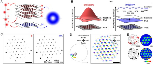
Model architecture and generation of 2D grid cells.
(A) Our model consists of a neural sheet with five overlapping populations, four of them excitatory—N, W, S, and E—and one inhibitory. Each density plot depicts the synaptic outputs in the sheet of a neuron at the origin. (B) Each neuron is driven to a particular membrane potential, which exceeds the spiking threshold for excitatory neurons at the center of the sheet and oscillates at 8 Hz for inhibitory neurons while the animal is running. (C) Snapshot of neural activity showing S and inhibitory populations separately; other excitatory populations have activity patterns similar to that of the S population. Each pixel is a neuron and dark colors indicate recent spiking. (D) Left, segment of a 2D open field trajectory. Right, neural activity over the course of the segment with each neuron colored according to the position at which it attained its maximum firing rate. Each attractor bump moves in synchrony with animal motion. (E) Left, two sample grid cells with spikes shown as colored dots superimposed on the animal’s trajectory. Each neuron’s location in the sheet is indicated by a circle of corresponding color in D. Right, autocorrelation of rate maps calculated from spikes at left. Black scale bars, 50 neurons. White scale bars, 50 cm.
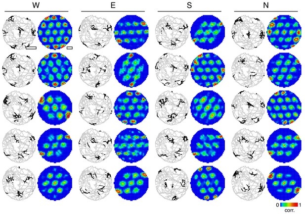
2D firing maps for many grid cells.
Spatial firing maps for a 2D open field trajectory. Twenty grid cells are selected from the simulation depicted in Figure 1D,E across all four excitatory populations. For each grid cell, spikes superimposed on the animal’s trajectory (left) and autocorrelation of rate maps calculated from spikes (right).
Emergence of a grid-like pattern on the neural sheet from randomly initialized membrane potentials.
Neural activities of the W and inhibitory populations over the first 240 ms of simulation setup. Each pixel is a neuron, with black corresponding to current spikes and lightest gray corresponding to spikes 40 ms ago. Defects in the grid are then removed as described in the Model details subsection of Appendix 1 before the main simulation begins.
Path integration over an open field trajectory produces 2D grid cells.
Left, neural activity of the W population. Each pixel is a neuron, with black corresponding to current spikes and lightest gray corresponding to spikes 40 ms ago. Red circle indicates the location of a single recorded neuron. Right, open field trajectory in an enclosure of diameter 1.8 m with a black square indicating the current animal position. Red dots indicate animal positions during spikes recorded from the neuron.
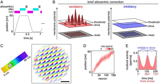
Grid cells along a 1D track.
(A) Trajectory consisting of runs along a track separated by idle periods at either end. Between the end of an idle period and the start of a run, the network receives brief allocentric input. (B) Allocentric input corrects the location of attractor bumps on the neural sheet (Materials and methods). (C) Left, track diagram. Right, neural activity over runs with each neuron colored according to the track position at which it attained maximum firing rate. Red circles indicate regions of recording. Scale bar, 50 neurons. (D) Firing fields of recorded grid cells sorted by position of maximum rate. (E) Multiunit activity of neurons in D averaged over theta cycles, which span from one trough of the oscillating inhibitory drive to the next. Data is repeated over two cycles for clarity.
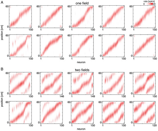
Firing fields for multiple simulations.
Firing fields of recorded grid cells along a 1D track. Fields are sorted by position of maximum rate. (A) Representative simulations exhibiting one field. (B) Representative simulations exhibiting two fields.
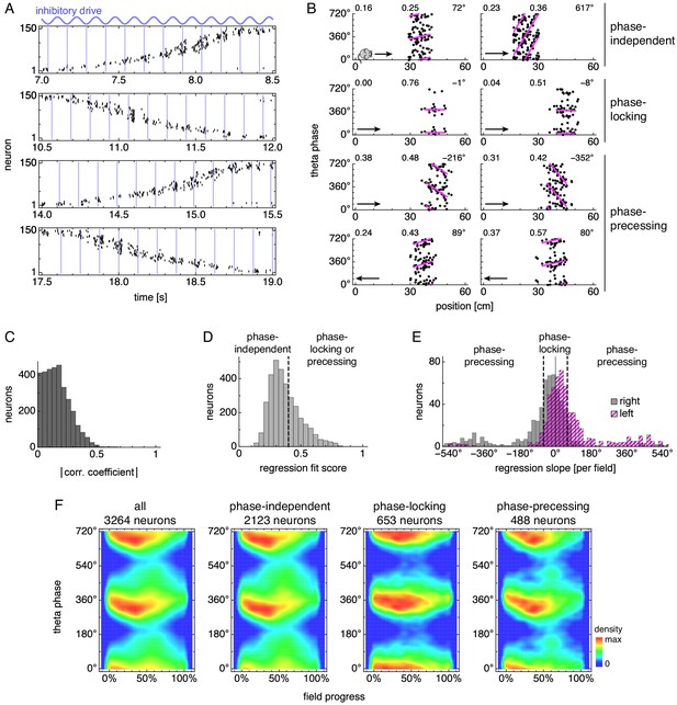
During runs, certain neurons exhibit theta phase locking and precession.
(A) Grid cell spike rasters for four laps along the track. Vertical blue lines indicate theta cycle boundaries. (B) Relationship between animal position along the track and theta phase for representative neurons. Dots represent spikes during runs in the directions indicated by arrows, with each spike repeated at two equivalent phases for clarity. Lines indicate fit by circular-linear regression. Numbers in each panel from top left to top right indicate magnitudes of correlation coefficients, regression fit scores, and regression slopes. (C–E) Data across all replicate simulations. (C) Magnitudes of circular-linear correlation coefficients. Mean ± s.d.: 0.17 ± 0.11. (D) Fit scores for circular-linear regression. (E) Regression slopes in units of field size for neurons with fit score >0.4. The predominance of negative values for rightward runs and positive for leftward runs indicates decreasing phase as the animal traverses grid fields in either direction. (F) Spike densities for different subgroups. An animal enters a grid field at progress 0% and exits it at 100%.
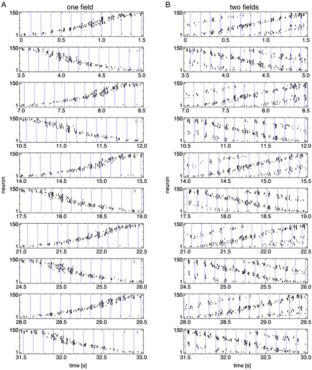
Spike rasters over multiple runs.
Vertical blue lines indicate theta cycle boundaries. (A) Representative simulation exhibiting one field. (B) Representative simulation exhibiting two fields.
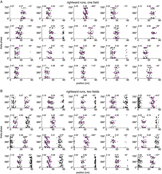
Position-phase relationships during rightward runs for many neurons.
Relationship between animal position along the track and theta phase during rightward runs. Dots represent spikes during runs in the directions indicated by arrows, with each spike repeated at two equivalent phases for clarity. Lines indicate fit by circular-linear regression. Numbers in each panel from top left to top right indicate magnitudes of correlation coefficients, regression fit scores, and precession ranges. (A) Representative neurons from simulations exhibiting one field. (B) Representative neurons from simulations exhibiting two fields.
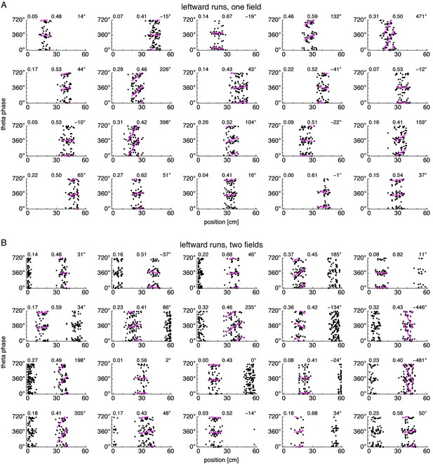
Position-phase relationships during leftward runs for many neurons.
Relationship between animal position along the track and theta phase during leftward runs. Panels same as in Figure 3—figure supplement 2.
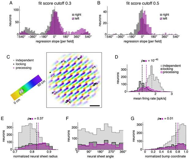
Further analysis of subgroups with different phase relationships.
Further analysis of subgroups of phase-independent, phase-locking, and phase-precessing neurons. (A,B) Distributions of regression slopes using a fit score cutoff different from 0.4, which was used in Figure 3. (C) Neural sheet locations of neurons belonging to each subgroup for the simulation described in Figure 3A,B. Data encompassing recording areas shown in Figure 2C and recording areas offset by 45° on the neural sheet. Left, track diagram. Right, neural activity over runs with each neuron colored according to the track position at which it attained maximum firing rate. Scale bar, 50 neurons. (D–G) Distribution of neurons in each subgroup with respect to various properties. Medians for each subgroup indicated by dashed lines. Medians for phase-locking and phase-precessing subgroups compared by the Mann-Whitney U test with reported p-value. (D) Mean firing rate. (E) Distance from the center of the neural sheet divided by the half the neural sheet size n. (F) Angle on the neural sheet relative to the right direction, or . (G) Location relative to attractor bumps in units of relative firing rate. A value of 1 means that the center of a bump passes over the neuron, and a value of 0 means that no part of a bump passes over the neuron (Appendix 1).
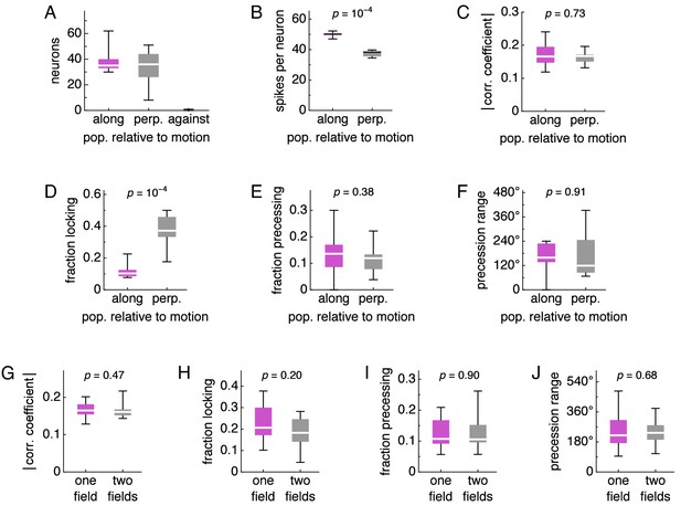
Dependence of phase relationships on excitatory population and number of fields.
Box-whisker plots with lines at medians, boxes between first to third quartiles, and whiskers between the entire data range excluding outliers lying more than 1.5 times the interquartile distance beyond the first or third quartile. Medians compared by the Mann-Whitney U test with reported p-values. (A–F) Analysis of phase relationships with respect to excitatory population. For these simulations, the direction of animal velocity is 0°, which means that runs are aligned to the E and W directions. The ‘along’ category corresponds to both the E population when the animal is running towards E and the W population when the animal is running towards W. The ‘against’ category corresponds to the E and W populations during the opposite running directions. The ‘perp.’ category corresponds to the N and S directions. (A) Number of valid recorded neurons. Note that there are very few ‘against’ neurons due to low firing rate, and this category is excluded from further analysis. (B) Number of spikes per neuron. (C) Magnitude of correlation coefficient. (D) Fraction of phase locking neurons. (E) Fraction of phase precessing neurons. (F) Phase precession range. (G–J) Analysis of phase relationships with respect to number of fields exhibited by a simulation. (G) Magnitude of correlation coefficient. (H) Fraction of phase locking neurons. (I) Fraction of phase precessing neurons. (J) Phase precession range.
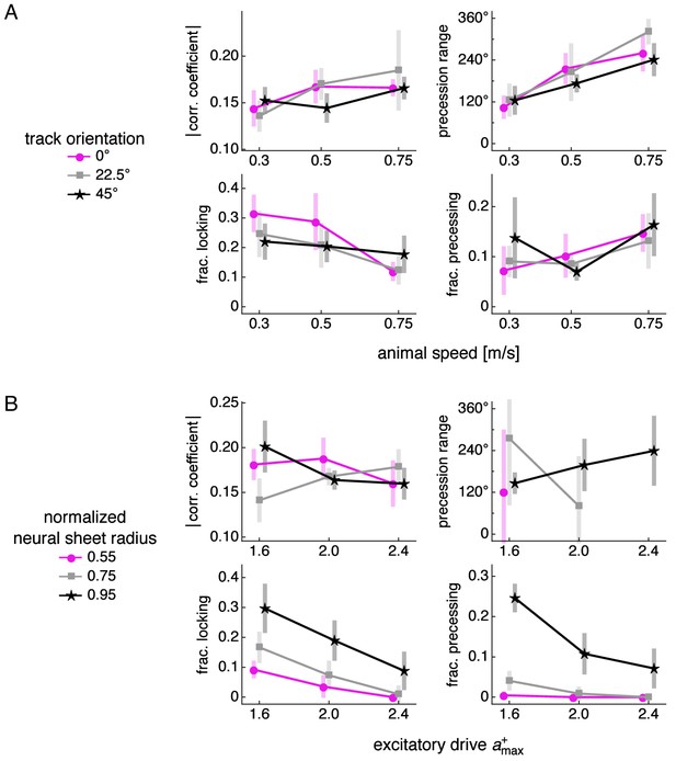
Phase relationship properties over different simulation parameters.
Correlation coefficient magnitude, precession range, fraction of phase-locking neurons, and fraction of precessing neurons as functions of various simulation parameters. Points at mean values with bars indicating s.d. over replicate simulations. Small horizontal offsets added for clarity. (A) Animal speed and track orientation relative to the E direction, or . (B) Excitatory drive and recording distance from the center of the neural sheet divided by the half the neural sheet size.
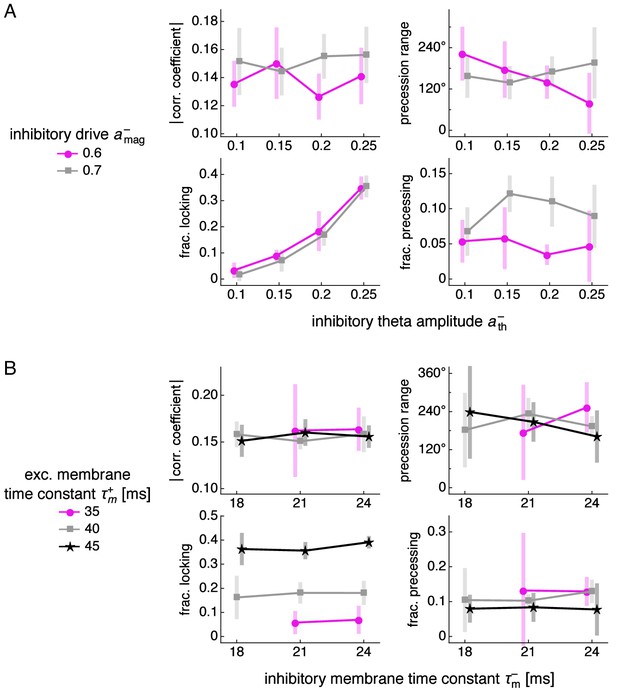
Phase relationship properties over different simulation parameters, continued.
Same as Figure 3—figure supplement 6, except as functions of different parameters. (A) Inhibitory theta amplitude and inhibitory drive. (B) Inhibitory and excitatory membrane time constants.
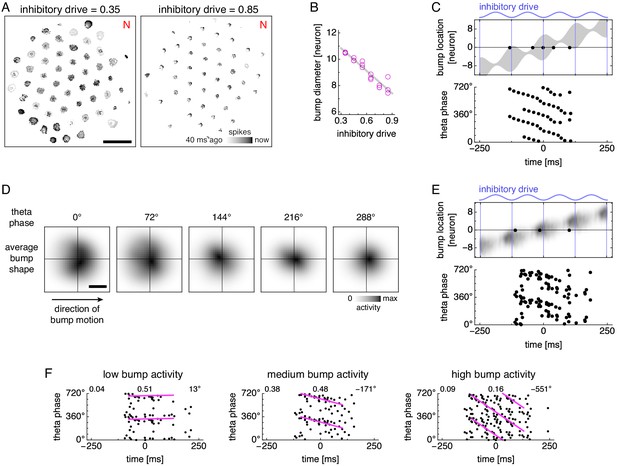
Bump size oscillations explain phase precession in models with simplified dynamics.
(A,B) Data from simulations with fixed inhibitory drive and constant animal velocity. (A) Snapshots of neural activity. Scale bar, 50 neurons. (B) The diameter of bumps on the neural sheet decreases linearly with inhibitory drive (linear regression , ANOVA ). (C) Phase precession in a conceptual model with bump size oscillations. We imagine an attractor bump, with size oscillations described by B, passing through a recorded grid cell. Top, a single lap. The recorded neuron is at location 0 and fires a spike (black dot) whenever contained within the bump (gray area), subject to a 40 ms refractory period. Bottom, relationship between theta phase and time across multiple laps with different initial phases. Spikes occur around 360° (equivalently, 0°) at the start of the field, and their phase generally decreases with time within in the grid field. (D) Attractor bump shape at different theta phases averaged over theta cycles and individual bumps (Appendix 1). Grays scaled separately for each theta phase. Scale bar, three neurons. (E,F) Phase behavior in a simplified model using average bump dynamics. (E) We imagine the average attractor bump passing through a recorded grid cell. Top, a single lap. The recorded neuron is at location 0 and stochastically fires a spike (black dot) with rate proportional to bump activity, subject to a 40 ms refractory period. Bottom, relationship between time and theta phase across multiple laps with different initial phases. (F) Relationship between time and theta phase using average bumps whose activity has been rescaled to different maximum values: 40, 50, and 100 spikes/s. Dots represent spikes generated according to E. Lines indicate fit by circular-linear regression. Numbers in each panel from top left to top right indicate magnitude of correlation coefficient, regression fit score, and regression slope.
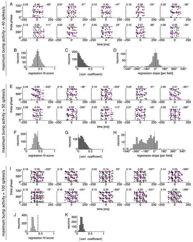
Simplified model using average bump dynamics produces different phase behaviors for different levels of rescaled activity.
Simplified model of phase precession using average bump dynamics. Bump activity is rescaled to different maximum values. (A–D) Neurons exhibit phase locking under low bump activity with maximum value 40 spikes/s. Statistics from 1000 neurons simulated according to Figure 4E. (A) Relationship between animal position along the track and theta phase for representative neurons. Dots represent spikes. Lines indicate fit by circular-linear regression. Numbers in each panel from top left to top right indicate magnitude of correlation coefficient, regression fit score, and regression slope. (B) Magnitudes of circular-linear correlation coefficients. (C) Fit scores for circular-linear regression. (D) Regression slopes for neurons with fit score >0.4. (E–H) Neurons exhibit phase precession under medium bump activity with maximum value 50 spikes/s. Panels same as A–D. (I–K) Neurons exhibit phase independence under high bump activity with maximum value 100 spikes/s. Panels same as A–C.
Phase precession in a simplified conceptual model.
An idealized attractor bump, with constant speed and oscillating size, passes through a recorded grid cell multiple times with different initial theta phases. This represents an animal running multiple laps in the same direction at constant speed. Top, the recorded neuron is at location 0 and fires a spike (black dot) whenever it is contained within the bump (gray area), subject to a 40 ms refractory period. Bottom, relationship between theta phase and time for spikes accumulated across multiple laps. Theta phase generally decreases with time within in the grid field. Since the simulated animal moves at constant speed, time is proportional to position, so theta phase decreases with position within in the grid field.
Average attractor bump shape as a function of theta phase.
Bump activity is averaged over multiple bumps and theta cycles. Darker areas indicate higher activity, scaled separately for each theta phase. The constant velocity component of bump motion is removed.
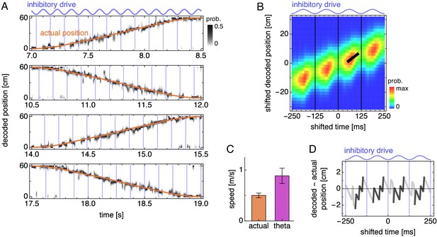
During runs, the decoded position exhibits theta sequences.
(A) Decoded position for four laps along the track corresponding to Figure 3A. Vertical blue lines indicate theta cycle boundaries. (B) Decoded position shifted by actual position and averaged over theta cycles. The thick black fit line indicates the time window with the steepest increase in decoded position. Vertical thin black lines indicate theta cycle boundaries. (C) Mean actual run speed (error bars indicate s.d. over time) and mean theta sequence speed, as indicated by the slope of the thick black line in B (error bars indicate s.d. over replicate simulations). (D) Difference between the maximum likelihood decoded position from B and the actual animal position as a function of time. Within each theta cycle, the segment from the smallest to the largest value is emphasized as a theta sequence.
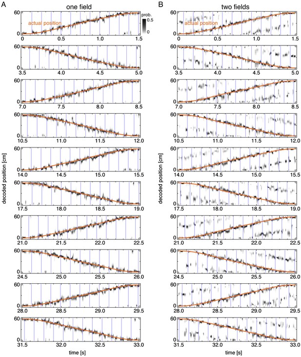
Decoded position over many runs.
Decoded position over multiple runs corresponding to Figure 3—figure supplement 1. Vertical blue lines indicate theta cycle boundaries. Orange line indicates the actual animal trajectory. (A) Representative simulation exhibiting one field. (B) Representative simulation exhibiting two fields.
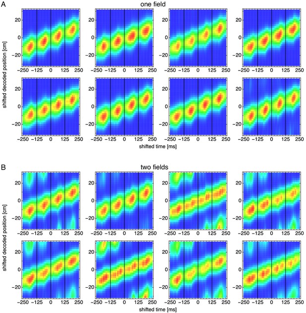
Decoded position shifted by actual position and averaged over theta cycles for many simulations.
Vertical black lines indicate theta cycle boundaries. (A) Representative simulations exhibiting one field. (B) Representative simulations exhibiting two fields.
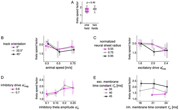
Dependence of theta sequence speed on number of fields and simulation parameters.
Theta sequence speed divided by mean actual speed for different numbers of fields and parameter values. (A) Dependence of theta speed on number of fields. Box-whisker plot with line at medians, box between first to third quartiles, and whiskers between the entire data range excluding outliers lying more than 1.5 times the interquartile distance beyond the first or third quartile. p-value calculated by the Mann-Whitney U test. (B–E) Theta sequence speed divided by mean actual speed as a function of various simulation parameters. Points at mean values with bars indicating s.d. over replicate simulations. (B) Animal speed and track orientation relative to the E direction, or . (C) Excitatory drive and recording distance from the center of the neural sheet divided by the half the neural sheet size. (D) Inhibitory theta amplitude and inhibitory drive. (E) Inhibitory and excitatory membrane time constants.
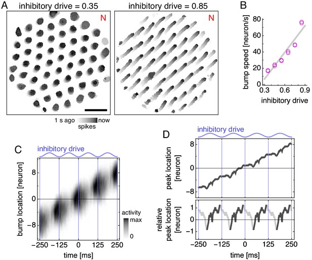
Bump speed oscillations explain theta sequences.
(A,B) Data from simulations with fixed inhibitory drive and constant animal velocity. (A) Snapshots of neural activity. Scale bar, 50 neurons. (B) The speed of bumps on the neural sheet increases linearly with inhibitory drive (linear regression , ANOVA ). Thus, the average decoded position in Figure 5B advances most rapidly around the middle of the theta cycle. (C) Activity of the average attractor bump depicted in Figure 4D along its central axis. (D) Top, peak activity location from C as a function of time. Bottom, peak activity position relative to constant bump motion as a function of time. Within each theta cycle, the segment from the smallest to the largest value is emphasized and corresponds to a theta sequence in Figure 5D.
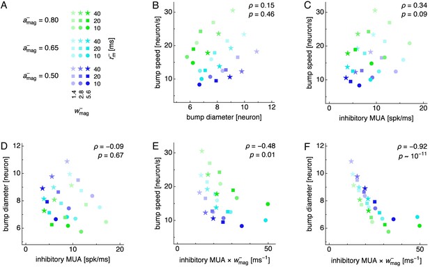
Relationship between attractor bump size and speed.
Attractor bump size and speed are not generally correlated over changes in multiple simulation parameters, but both are negatively correlated with the amount of inhibition produced by inhibitory neurons. (A) Legend for simulations with fixed inhibitory drive. Each simulation is performed at different values of inhibitory drive , inhibitory synaptic strength , and inhibitory membrane time constant . Other parameters are set at the values used for main simulation runs (Table 1). (B–F) Relationships between pairs of attractor bump properties across parameters displayed in A. Rank correlation computed by Spearman’s with p-values indicated. Attractor bump properties are diameter, speed, the multiunit activity of inhibitory neurons (inhibitory MUA), and a metric for the amount of inhibition produced by inhibitory neurons (). Note that B indicates no overall correlation between bump size and speed, but increasing (following blue–cyan–green) increases bump speed and decreases bump diameter, as seen in Figure 4B and Figure 6B.
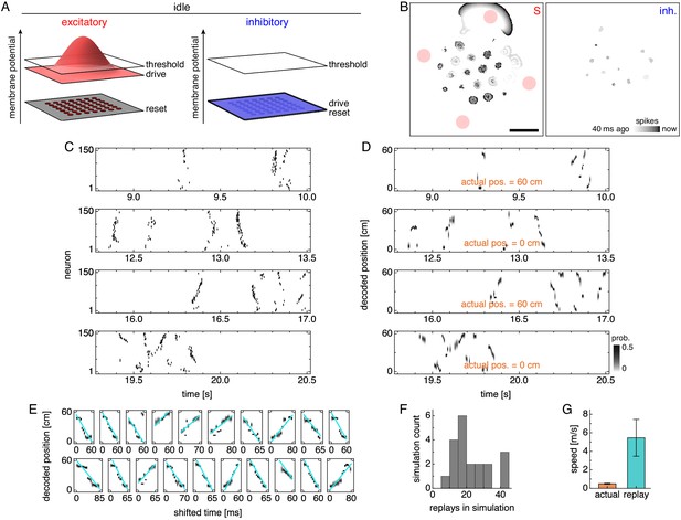
Lower drive during quiescence produces traveling wavefronts of activity that are decoded as replays.
(A) During idle periods at either end of the track, excitatory and inhibitory drives decrease, and the latter no longer oscillates. (B) Snapshot of neural activity showing S and inhibitory populations separately. Red circles indicate regions of recording. Scale bar, 50 neurons. (C) Grid cell spike rasters for four idle periods. (D) Decoded position corresponding to C. Rapid trajectory sweeps arise from traveling wavefronts as depicted by the S population in B. (E) Replays from one simulation with cyan fit lines. (F) Number of replays across simulations. (G) Mean actual run speed (error bars indicate s.d. over time) and mean replay speed, as indicated by the slopes of cyan lines in E (error bars indicate s.d. over replays).
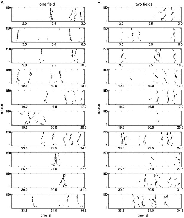
Spike rasters over multiple idle periods.
(A) Representative simulation exhibiting one field. (B) Representative simulation exhibiting two fields.
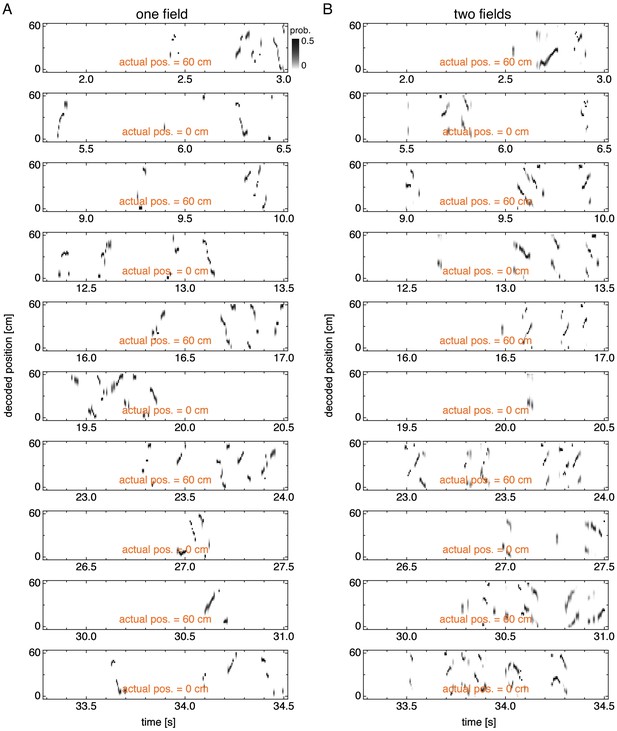
Decoded position over many idle periods.
Decoded position over multiple idle periods corresponding to Figure 7—figure supplement 1. (A) Representative simulation exhibiting one field. (B) Representative simulation exhibiting two fields.
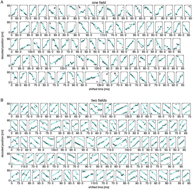
Many replays.
Replays with cyan fit lines. (A) Representative replays from simulations exhibiting one field. (B) Representative replays from simulations exhibiting two fields. Note that two or three parallel lines participate in the fit (Appendix 1).
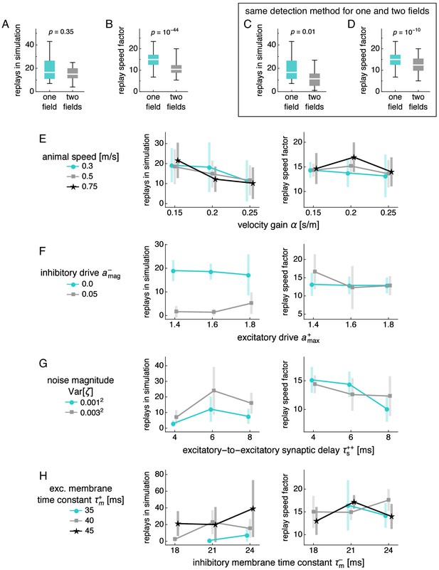
Dependence of replay count and speed on number of fields and simulation parameters.
(A–D) Dependence of replay count and speed on number of fields. Box-whisker plot with line at medians, box between first to third quartiles, and whiskers between the entire data range excluding outliers lying more than 1.5 times the interquartile distance beyond the first or third quartile. p-value calculated by the Mann-Whitney U test. (A) Replay count. (B) Replay speed divided by mean actual speed. (C,D) Same as A,B, but we detect replays in simulations exhibiting two fields with the same method used for single fields. (E–H) Replay count and replay speed divided by mean actual speed as functions of various simulation parameters. Points at mean values with bars indicating s.d. over replicate simulations. (E) Velocity gain and animal speed. (F) Excitatory and inhibitory drive. (G) Excitatory-to-excitatory synaptic delay and noise magnitude for both excitatory and inhibitory neurons. (H) Inhibitory and excitatory membrane time constants.
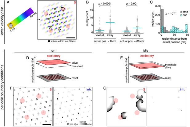
Replays acquire additional properties in networks with different configurations of attractor bumps.
(A–C) With lower velocity gain, neural sheet locations have a clear one-to-one correspondence with track positions, which allows replays to exhibit a directional bias. (A) Left, track diagram with animal idle at 0 cm. Right, corresponding snapshot of neural activity superimposed on a background colored according to the position at which each neuron attains its maximum firing rate (cf. Figure 2C, right panel). Red circles indicate regions of recording. Attractor bumps still represent the animal position, and a wavefront can be seen emanating from one bump at the top right. (B) Direction of replay propagation across simulations. For each actual position and replay direction, width of gray bars indicates the number of simulations with a particular replay count. Means indicated with lines. p-values from the Mann-Whitney U test show that a significantly greater number of replays propagate away from either actual position. (C) Distances between actual position and decoded position at the start or end of replays. Paired medians compared by the Wilcoxon rank-sum test with indicated p-value. (D–G) With periodic boundary conditions and uniform excitatory drive, attractor bumps and activity wavefronts appear throughout the neural sheet. (D,E) Excitatory drive during runs and idle periods. (F,G) Snapshots of neural activity during runs and idle periods showing S and inhibitory populations. Each pixel is a neuron and dark colors indicate recent spiking. Red circles indicate regions of recording. Scale bars, 50 neurons.
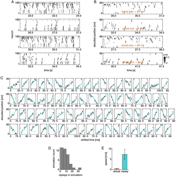
Replay properties in simulations with lower velocity gain.
(A) Grid cell spike rasters for four idle periods. (B) Decoded position corresponding to A. (C) Replays across multiple simulations with cyan fit lines. (D) Number of replays across simulations. (E) Actual run speed 0.50 ± 0.05 m/s (mean ± s.d. over time) and replay speed 7.4 ± 2.3 m/s (mean ± s.d. over replays).
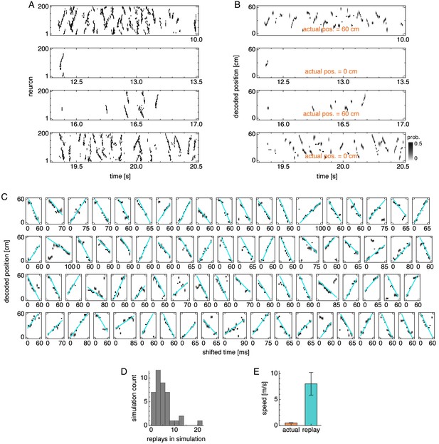
Replay properties in simulations with periodic boundary conditions and uniform excitatory drive.
Same as Figure 8—figure supplement 1, but for simulations with periodic boundary conditions and uniform excitatory drive. Replay speed is 8.0 ± 2.2 m/s (mean ± s.d. over replays).
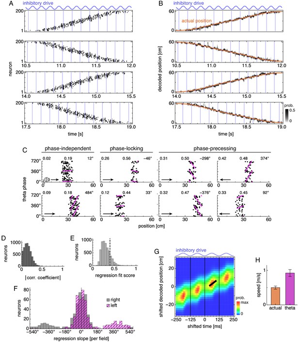
Phase precession and theta sequence properties in simulations with periodic boundary conditions and uniform excitatory drive.
(A) Grid cell spike rasters for four runs. Vertical blue lines indicate theta cycle boundaries. (B) Decoded position corresponding to A. (C) Relationship between animal position and theta phase for representative neurons. Dots represent spikes during runs in the directions indicated by arrows. Lines indicate fit by circular-linear regression. Numbers in each panel from top left to top right indicate magnitudes of correlation coefficients, regression fit scores, and regression slopes. (D–F) Data across all replicate simulations. (D) Magnitudes of circular-linear correlation coefficients. Mean ± s.d.: 0.14 ± 0.09. (E) Fit scores for circular-linear regression. (F) Regression slopes for neurons with fit score >0.4. (G) Decoded position averaged over theta cycles. Thick black line fit to theta sequence. (H) Actual run speed 0.50 ± 0.05 m/s (mean ± s.d. over time) and theta sequence speed 0.90 ± 0.11 m/s (mean ± s.d. over replicate simulations).
Replays preferentially radiate from attractor bumps encoding the current animal position.
The activity snapshot in Figure 8A corresponds to t = 41.14 s. Left, position of the animal (black square) at 0 cm along a 1D track, whose positions are colored with a gradient. Right, neural activity of the E population superimposed upon a spatial firing map. Each neuron is colored according the position at which it attains maximum firing rate. Each black pixel represents a spike within the last 5 ms. A wavefront travels through the red recording region located at the top right of the neural sheet. It emanates from an attractor bump sustained by yellow neurons that represent the current position of 0 cm, and it rapidly sweeps through neurons representing progressively farther track positions.
Neural activity during runs, idle periods, and allocentric corrections for a simulation with periodic boundary conditions and uniform excitatory drive.
Left, position of the animal (black square) along a 1D track. Right, neural activity of the E population. Each pixel is a neuron, with black corresponding to current spikes and lightest gray corresponding to spikes 40 ms ago. Red circles indicate regions of recording.
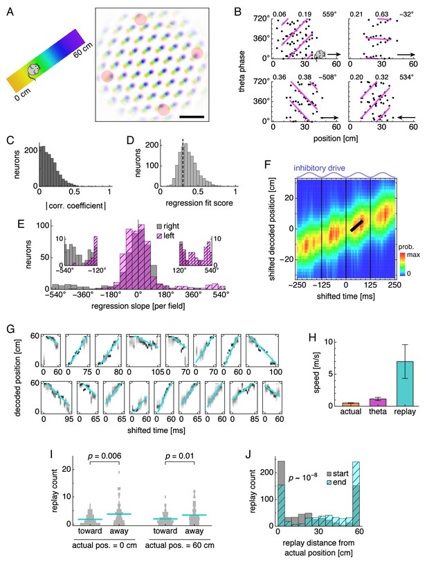
Theta-related and replay properties in simulations without brief allocentric corrections.
(A) Left, track diagram. Right, neural activity over runs with each neuron colored according to the track position at which it attained maximum firing rate. Red circles indicate regions of recording. (B) Relationship between animal position and theta phase for representative neurons. Clockwise from top left, relationships depicted are phase independence, phase locking, phase precession, and phase precession. Dots represent spikes during runs in the directions indicated by arrows. Lines indicate fit by circular-linear regression. Numbers in each panel from top left to top right indicate magnitudes of correlation coefficients, regression fit scores, and precession ranges. (C–E) Data across all replicate simulations. (C) Magnitudes of circular-linear correlation coefficients. Mean ± s.d.: 0.15 ± 0.11. (D) Fit scores for circular-linear regression. (E) Regression slopes for neurons with fit score >0.3. (F) Decoded position averaged over theta cycles. Thick black line fit to theta sequence. (G) Replays with cyan fit lines. (H) Mean actual run speed (error bars indicate s.d. over time), mean theta sequence speed (error bars indicate s.d. over replicate simulations), and mean replay speed (error bars indicate s.d. over replays). (I) Direction of replay propagation across simulations. Means indicated with lines. p-values from the Mann-Whitney U test show that a significantly greater number of replays propagate away from either actual position. (J) Distances between actual position and decoded position at the start or end of replays. Paired medians compared by the Wilcoxon rank-sum test with indicated p-value. Scale bars, 50 neurons.
Videos
Neural activity during runs, idle periods, and allocentric corrections.
Left, position of the animal (black square) along a 1D track. Right, neural activity of the E population. Each pixel is a neuron, with black corresponding to current spikes and lightest gray corresponding to spikes 40 ms ago. Red circles indicate regions of recording.
Neural activity during runs and idle periods during a simulation without allocentric corrections.
Left, position of the animal (black square) along a 1D track. Right, neural activity of the E population. Each pixel is a neuron, with black corresponding to current spikes and lightest gray corresponding to spikes 40 ms ago. Red circles indicate regions of recording.
Tables
Main model parameters and their values unless otherwise noted.
Values that change between runs, idle periods, and allocentric corrections are indicated accordingly.
| Parameter | Variable | Value |
|---|---|---|
| Neurons per population | ||
| Simulation timestep | 1 ms | |
| Exc. membrane time constant | 40 ms | |
| Inh. membrane time constant | 20 ms | |
| Exc.-to-exc. synaptic delay | 5 ms | |
| Exc.-to-inh. synaptic delay | 2 ms | |
| Inh. synaptic delay | 2 ms | |
| Exc. drive maximum | ||
| Exc. drive minimum | 0.8 | |
| Exc. drive scaled spread | ||
| Inh. drive magnitude | ||
| Inh. drive theta amplitude | ||
| Inh. drive theta frequency | 8 Hz | |
| Exc. synaptic strength | 0.2 | |
| Exc. synaptic spread | 6 | |
| Inh. synaptic strength | 2.8 | |
| Inh. synaptic distance | 12 | |
| Exc. synaptic shift | 3 | |
| Exc. velocity gain | 0.25 s/m | |
| Exc. noise magnitude | 0.0022 | |
| Inh. noise magnitude | 0.0022 |
Additional files
-
Source code 1
Source code for the main simulation written in C.
- https://cdn.elifesciences.org/articles/46351/elife-46351-code1-v2.zip
-
Transparent reporting form
- https://cdn.elifesciences.org/articles/46351/elife-46351-transrepform-v2.docx


