Self-organised segregation of bacterial chromosomal origins
- Heidelberg University, Germany
- University of Oxford, United Kingdom
- Max Planck Institute for Terrestrial Microbiology, LOEWE Centre for Synthetic Microbiology (SYNMIKRO), Germany
Figures
Figure 1 with 1 supplement

Fluorescence microscopy indicates that ori and MukBEF are not positioned independently of one another.
A strain with FROS (LacI-mCherry) labelled ori and MukB-mYPet was treated with DL serine hydroxamate to obtain cells with a single non-replicating chromosome and imaged at 1 min intervals. (a) Overlay of phase contrast and fluorescence images showing three representative cells. Bar indicates 2 µm. (b) The position distribution (along the long axis of the cell) of fluorescent foci of ori (red) and MukB (blue). N = 31820 from 952 cells tracked over up to 56 frames. Cells have a mean length of 2.2 µm. (c) The expected distribution (dashed line) of the distance between ori and MukB foci given that the distributions in (b) are independent. The measured distribution (circles and solid line) of separation distances from the same cells. (d) The step-wise velocity of ori as a function of position relative to mid-cell (blue) and to the MukB focus (red). (e) The step-wise velocity of MukB as a function of position relative to mid-cell (blue) and the ori (red). Shaded regions indicate standard error. See also Figure 1—figure supplement 1.
-
Figure 1—source data 1
Matlab .mat files containing the data used in Figure 1.
- https://doi.org/10.7554/eLife.46564.004
Figure 1—figure supplement 1
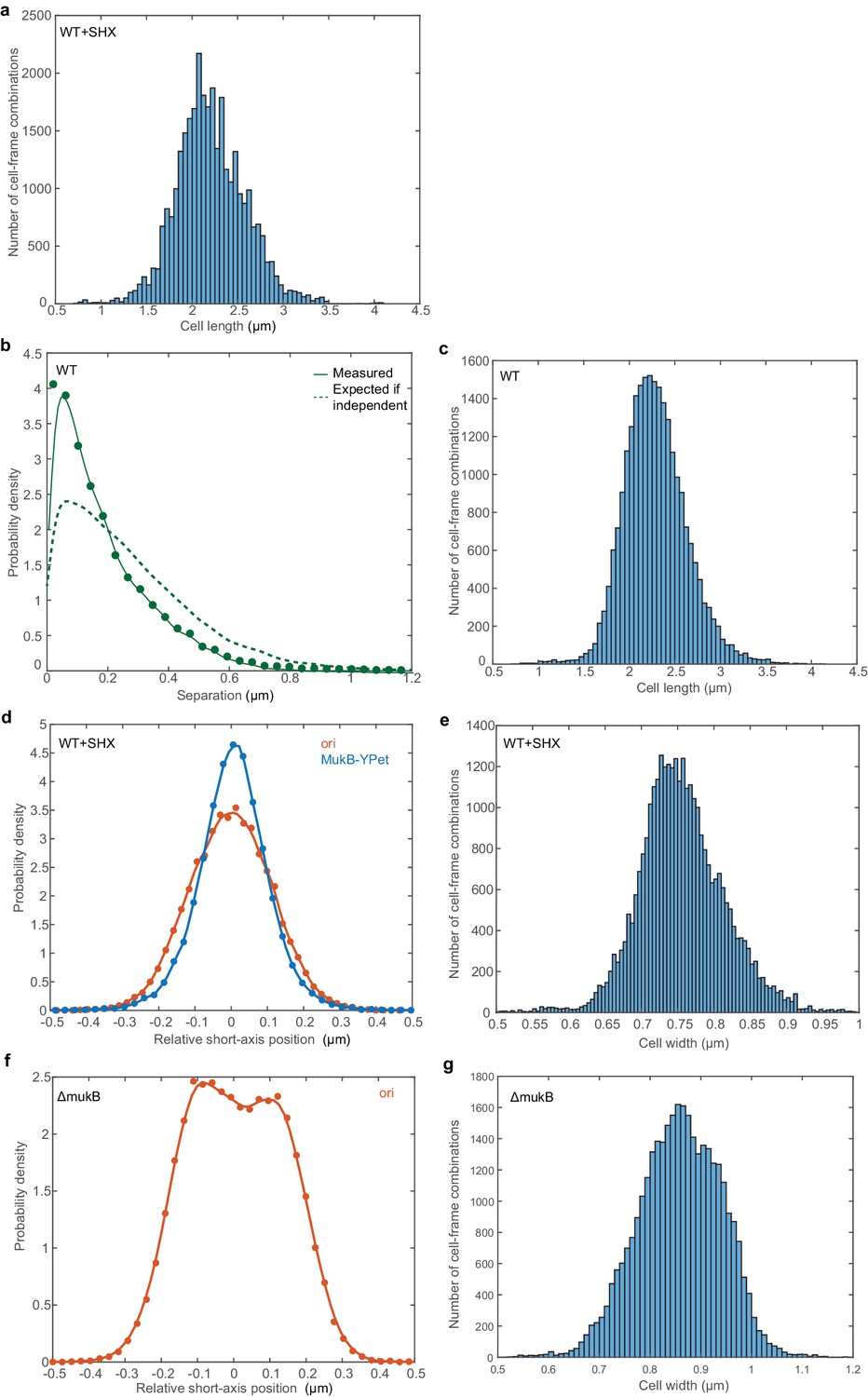
Positioning of ori (LacI-mCherry) and MukB-mYPet foci.
(a) Histogram of cell lengths of the cells analysed in Figure 1b,c. The mean cell length is 2.2 µm. (b) The predicted and measured distributions of the distance between ori and MukB-mYPet foci (in cells with a single focus of each) as in Figure 1c but without treatment with SHX. N = 16961 from 2401 cells imaged every five mins. (c) Histogram of cell lengths of the cells analysed in (b). The mean cell length is 2.2 µm. (d) The relative position distribution along the short axis of the cell for the same cells analysed in Figure 1 and (a). 95% of ori foci are within the centre 44% of the cell width, corresponding to a region 0.33 µm wide. 95% of MukB-mYPet foci are within the centre 39% of the cell width, corresponding to a region 0.30 µm wide. Note that the centre 40% region consists of 50% of the cross-sectional area. (e) Histogram of cell widths of the cells analysed in (d). The mean cell width is 0.756 µm. (f) The relative position distribution of ori along the short axis of the cell in cells lacking MukB. (a). 95% of ori foci are within the centre 50% of the cell width, corresponding to a region 0.42 µm wide. The centre 50% region consists of 61% of the cross-sectional area. N = 33001 from 1190 cells imaged every minute. (g) Histogram of cell widths of the cells analysed in (f). The mean cell width is 0.859 µm.
Figure 2 with 5 supplements
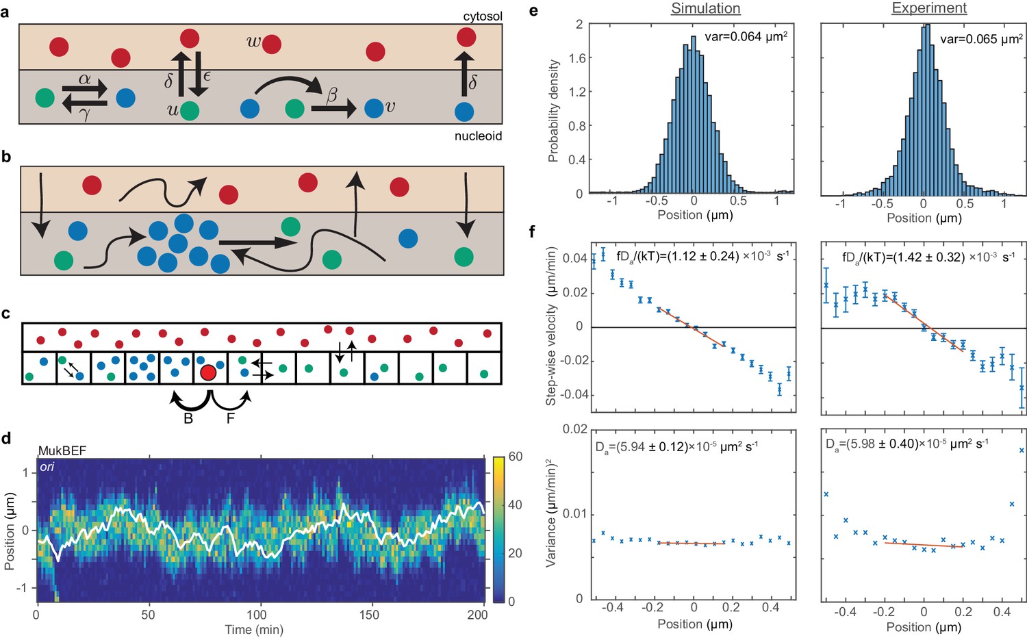
ori positioning by a self-organised protein gradient reproduces experimental results.
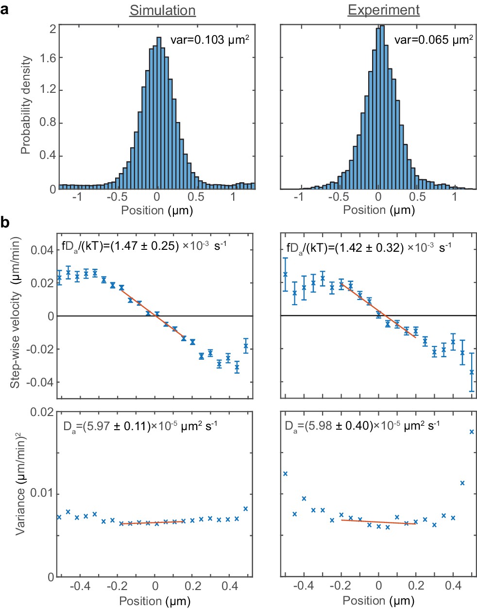
(a) Schematic showing the reactions of the previous MukBEF model (Murray and Sourjik, 2017) (see methods). Species w diffuses in the cytosol (red). Species u (green) and v (blue) diffuse on the nucleoid. Binding and species interaction are indicated by arrows. Diffusion is not shown. See the methods for a review of the model and the model parameters. (b) Schematic showing the flux-balance mechanism. The thinner arrows represent binding/unbinding and diffusion. Species w (red) is well-mixed and therefore converts to species u (green) uniformly across the nucleoid. If a molecule of species u explores a sufficiently large region of the nucleoid before it detaches again, then the flux of u molecules reaching a high density region (focus) of species v (blue) from either side is proportional to the length of the nucleoid on either side. This difference in fluxes leads to net movement of the self-organised focus towards the position at which the fluxes balance, the mid-cell in the case of a single focus. (c) The stochastic model is implemented using the spatial Gillespie method which discretises the spatial dimension into compartments in which molecules react and between which molecules can diffuse. Colours label species as in (a). The cytosolic species is taken to be well-mixed and its concentration is therefore not simulated spatially. This is the same implementation as was used previously (Murray and Sourjik, 2017). In this work, we extend these simulations by incorporating the ori as a single diffusing particle (outlined red circle). However, unlike MukBEF its diffusion is biased, being determined by forward (F) and backward (B) jump rates that depend on the gradient of MukBEF concentration (blue circles, v) (see methods). (d) Kymograph from a single simulation showing the number of MukBEF molecules (colour scale) and the position of the ori (white line). (e) and (f) A comparison between the experimental data of Kuwada et al. (2013) and the results of simulations in the case of a single ori and 6x preferential loading. (e) Histograms of ori position (unscaled) along the long axis of the cell. Zero is the middle position. (f) Mean (top) and variance (bottom) of the step-wise velocity as a function of position relative to mid-cell. Bars indicate standard error. The linear velocity profile at mid-cell is indicative of diffusion in a harmonic potential (). In such a model the variance of the step-wise velocity is independent of position. Thus we obtain the apparent diffusion constant and drift rate by fitting to the central region. Bounds are 95% confidence intervals. Red lines are weighted linear fits. Simulated data are from 100 independent runs, each of 600 min duration. Experimental data are based on over 16000 data points from 377 cells. Both data sets use 1 min time-intervals. Simulations are from 2.5 μm cells, whereas experimental data is from a range of cell lengths. See methods for further details and model parameters. See also Figure 2—figure supplement 1–5.
Figure 2—figure supplement 1
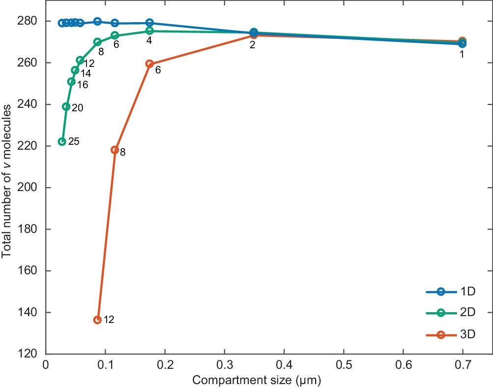
Compartment size effects.
The total number of v molecules as a function of compartment size in one, two and three dimensions. Simulations were performed as in Figure 2d but without ori and with a cell length of 2.8 µm. The width of the simulated rectangle (2D), rectangular cuboid (3D) is 0.7 µm. Individual compartments are square (2D) or cubic (3D). The number of compartments along the short axis is overlayed for 2D and 3D. The number of compartments along the long axis is four times this number.
Figure 2—figure supplement 2
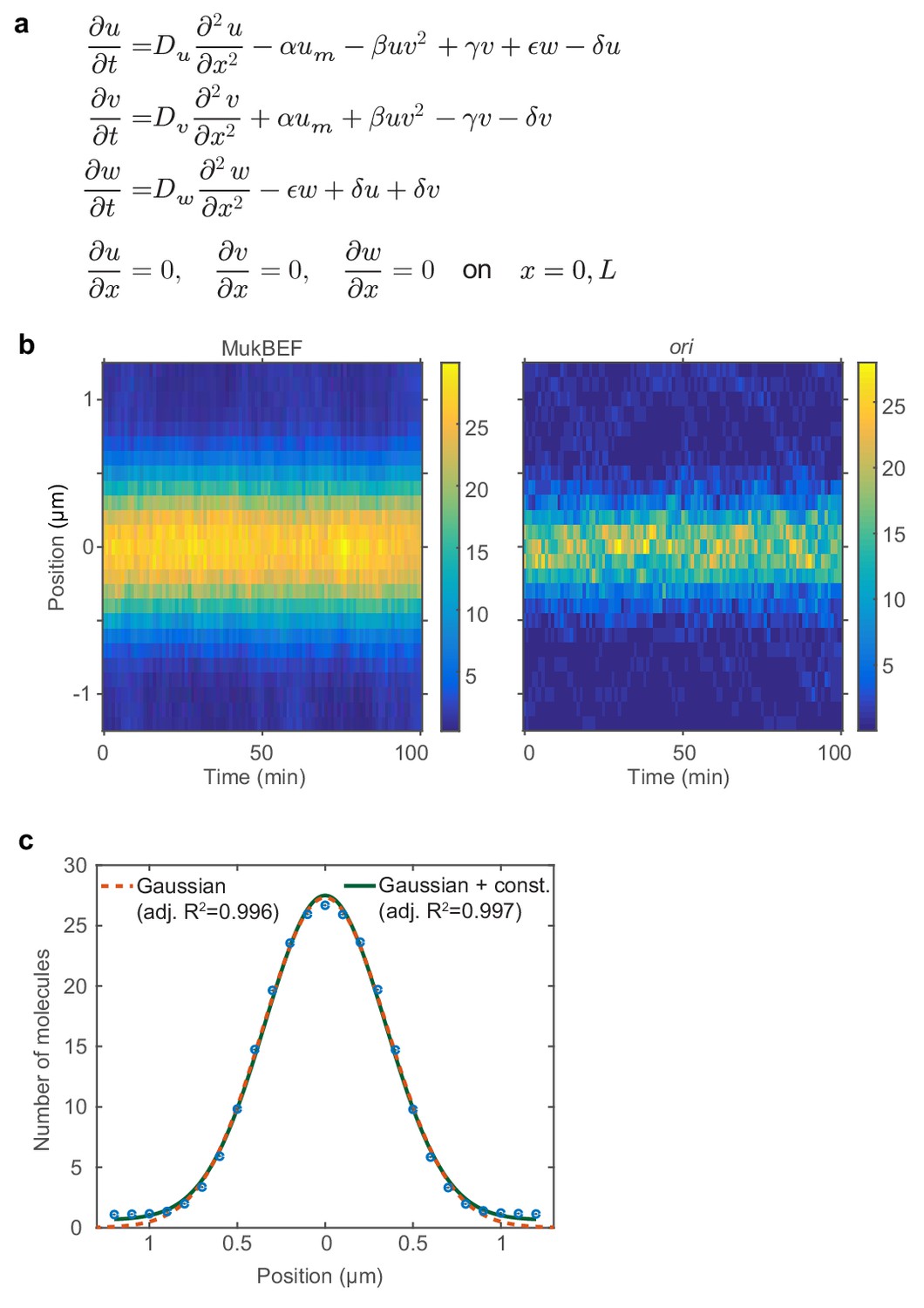
Properties of MukBEF model and ori positioning.
(a) The differential equations of the model in Figure 2a. Given for reference and to specify the nature of the reaction terms. In this work, we exclusively use the stochastic implementation of the model (Figure 2c). (b) Average kymographs from 100 simulations showing the distributions of MukBEF and ori positions. (c) The average MukBEF profile in the simulations (blue dots) is well approximated by a Gaussian.
Figure 2—figure supplement 3
Fitting the model to experimental data.
A fit to the experimental data of Kuwada et al. (2013) and the results of simulations in the case of a single ori (without preferential loading). (a) Histograms of ori position (unscaled) along the long axis of the cell. Zero is the middle position. (b) Mean (top) and variance (bottom) of the step-wise velocity as a function of position relative to mid-cell. Bars indicate standard error. The linear velocity profile at mid-cell is indicative of diffusion in a harmonic potential (). In such a model the variance of the step-wise velocity is independent of position. Thus we obtain the apparent diffusion constant and drift rate by fitting to the central region. Bounds are 95% confidence intervals. Red lines are weighted linear fits. Simulated data are from 100 independent runs, each of 600 min duration. Experimental data are based on over 16000 data points from 377 cells. Both data sets use 1 min time-intervals. Simulations are from 2.5 μm cells, whereas experimental data is from a range of cell lengths.
Figure 2—figure supplement 4
Additional properties in short cells with one ori.
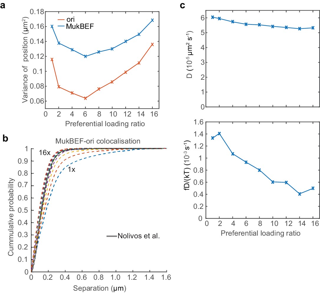
(a) The variance of the MukBEF and ori position distributions for different preferential loading ratios for the case of a single ori. (b) Cumulative probability distribution of the separation distance between ori and MukBEF peaks. (c) The change in the apparent diffusion constant and drift rate as a function of the preferential loading rate.
Figure 2—figure supplement 5
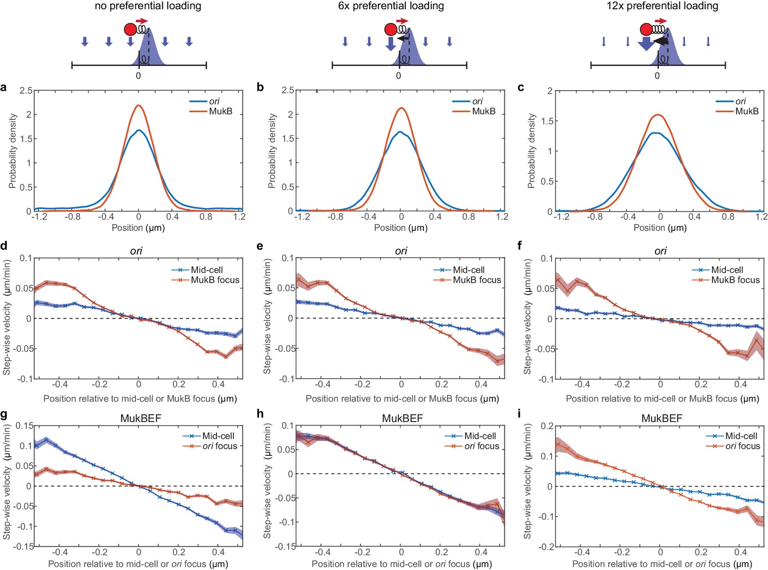
MukBEF is attracted towards mid-cell at low loading ratios and towards ori at high loading ratios.
(a–c) Simulated position distributions of MukBEF and ori for no (a), six times (b) and 12 (c) times preferential loading. The MukBEF position is the centroid of the simulated MukBEF peak. (d–i) Simulated step-wise ori (d–f) and MukBEF velocities (g–i) for no (d,g), six times (e,h) and 12 (f,i) times preferential loading as above. Shaded region indicates standard error. Note the inversion in the dominant MukBEF restoring velocity as preferential loading is increased. The position distribution and ori step-wise velocity for the case of no preferential loading are reproduced from Figure 2—figure supplement 3. Note that MukBEF is not affected by ori in the absence of preferential loading. The apparent restoring velocity of MukBEF towards ori in (g) is not physical and is likely due to the higher variability (diffusivity) of the MukBEF focus compared to ori.
Figure 3 with 1 supplement
Preferential loading of MukBEF at ori leads to correct and stable partitioning.
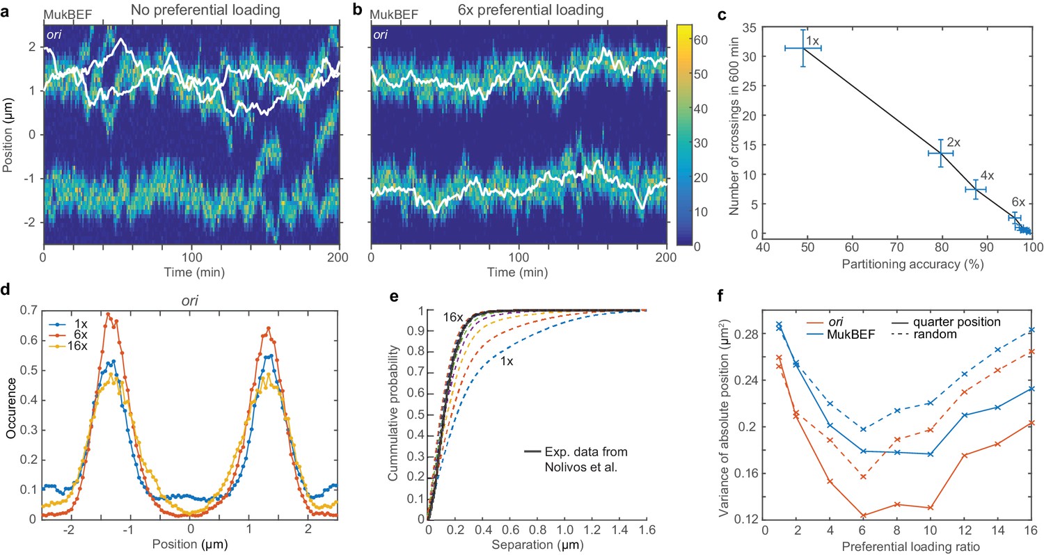
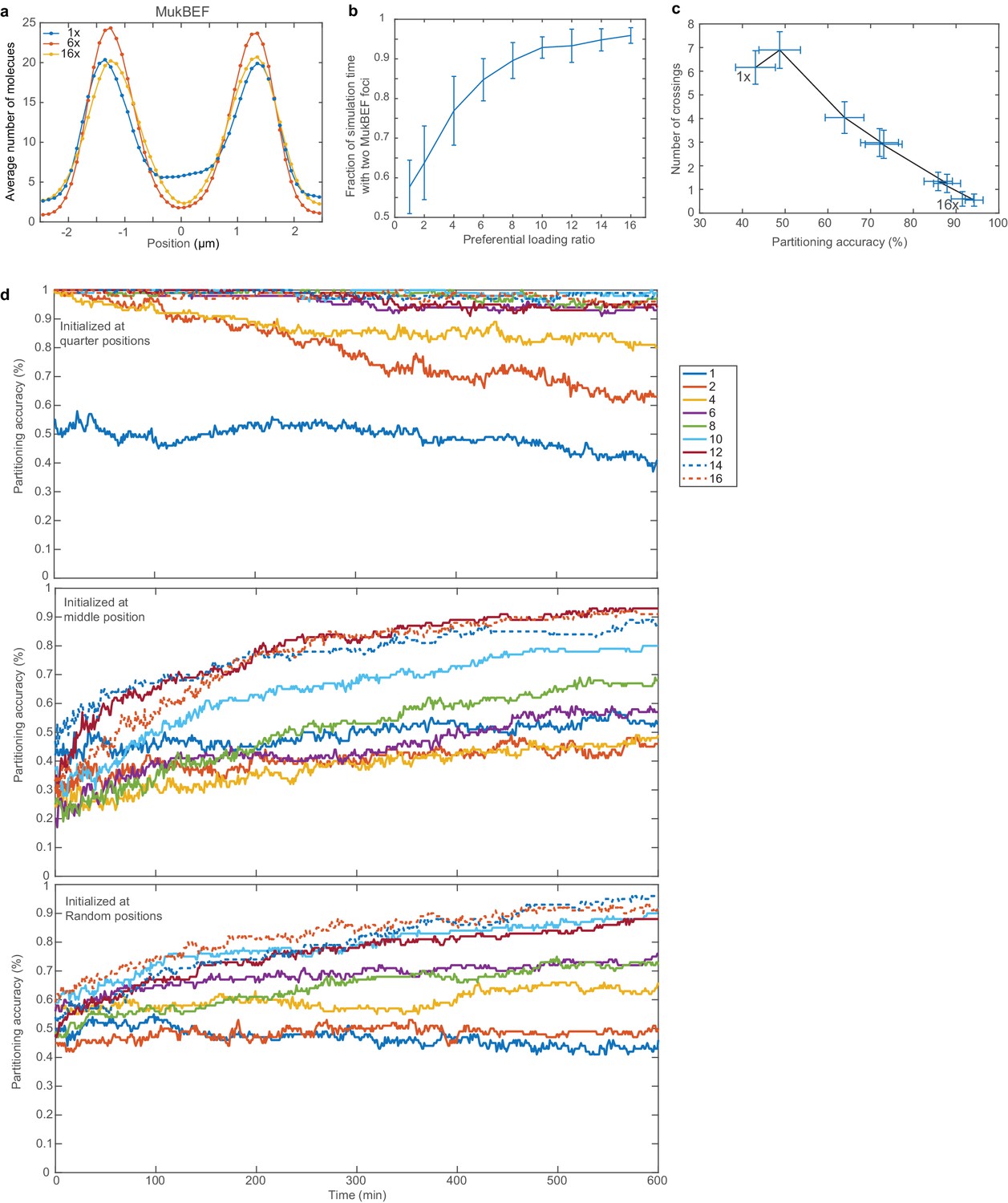
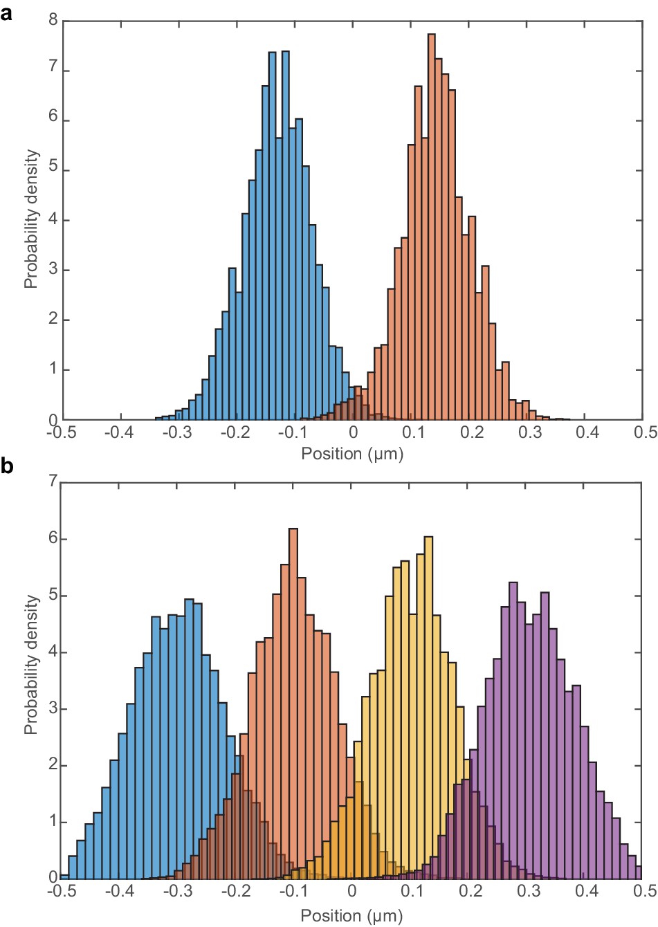
(a) Example simulated kymograph showing two ori (white lines) diffusing around the same MukBEF peak (colour scale). This occurs approximately 50% of the time. (b) The addition of 6x preferential loading of MukBEF at ori positions results in correct partitioning of ori. The loading rate in each of the spatial compartments containing ori is six times that of the other 48 compartments. The total loading rate is unchanged. (c) Partitioning accuracy is measured by the fraction of simulations with ori in different cell halves. Stability is measured by the number of times ori cross paths. Both partitioning accuracy and stability increase with preferential loading up to approximately 6x. Preferential loading ratios are as in (f). Points and bars indicate mean and standard error over independent simulations. See also Figure 3—figure supplement 1c. (d) Histograms of ori positions for 1x, 6x and 16x preferential loading. Positioning is more precise at 6x than with no or 16x preferential loading. See Figure 3—figure supplement 1a for MukBEF distributions. (e) The cumulative probability distribution for the separation distance between ori and MukBEF peaks. Experimental data (black line) is from Nolivos et al. (2016). The addition of preferential loading leads to substantially better agreement. Preferential loading ratios are as in (f). See also Figure 2—figure supplement 4b. (f) The variances of individual peaks (obtained by reflecting the data around the mid-position) have a minimum at approximately 6x preferential loading. Solid lines are from simulations with ori initially at the quarter positions, as for (a)-(e). Dashed lines are from simulations with random initial ori positions. Simulations were performed for a 5 µm domain and two ori.
Figure 3—figure supplement 1
Additional properties of model in longer cells with two ori.
(a) Histograms of MukBEF numbers for 1x, 6x and 16x preferential loading. Positioning is more precise at 6x than with no or 16x preferential loading. (b) Fraction of simulation time with two MukBEF foci as a function of the preferential loading ratio. Error bars indicate standard deviation. (c) Partitioning accuracy and stability as in Figure 3c but using random initial ori positions. Data is from the last 100 min of 600 min simulations. Due to both ori sometimes being in close initial proximity, the occurrence of the undesirable configuration (both ori associated to the same MukBEF peak) is higher. Nevertheless the system eventually tends to transition (irreversibly) to the correct configuration, promoted by high preferential loading rates. The loading ratios are as in (b). (d) Partitioning accuracy as a function of time and preferential loading ratio for different initial ori positions. Note that simulations were run for 30 min. before the system state was recorded in order to allow the self-organised MukBEF profile to establish and stabilise. Hence, ori have already moved from their initial positions at the first recorded time-point.
Figure 4 with 3 supplements
Repulsion between newly replicated ori results in realistic simulations of growing cells.
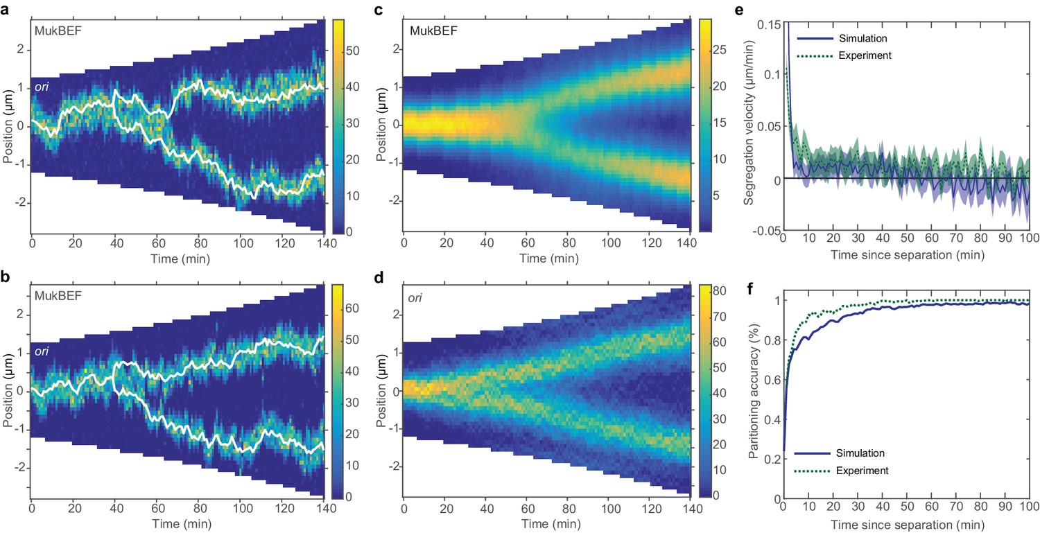
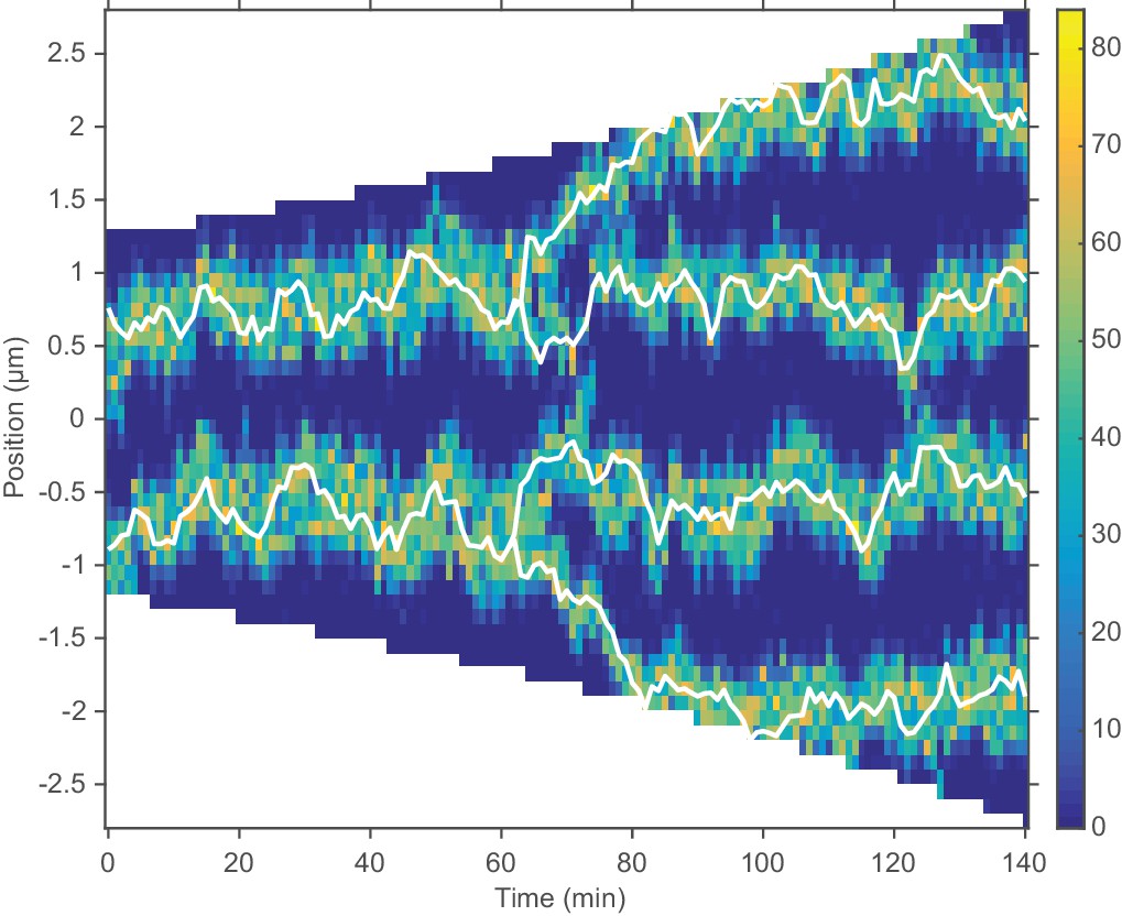
(a) and (b) Two example kymographs from individual simulations during exponential growth (doubling time of 120 min) in the presence of a repulsive force between ori. Shown is the number of MukBEF molecules (colour scale) overlayed with the ori position (while lines). (c) and (d) Average kymographs of MukBEF (c) and ori position (d). (e) and (f) Segregation velocity (the step-wise rate of change of the absolute distance between ori) (e) and partitioning accuracy (f) plotted as function of the time since ori duplication (simulations, blue) or separation (experiment, green). Experimental data is from Kuwada et al. (2013). Shading indicates 95% confidence intervals. The segregation velocity has been corrected for growth. Simulation results in (c–f) are from 450 independent simulations and use 10x preferential loading ratio and a repulsion range of 200 nm (as indicated by the black circle in Figure 4—figure supplement 2).
Figure 4—figure supplement 1

The effect of preferential loading during growth.
(a) Two randomly selected individual simulations of exponential growth with homogeneous loading. The colour scale represents the number of MukBEF molecules; white lines show the positions of ori. (b) Average kymograph of the number of MukBEF molecules (top) and ori positions (bottom). (c) and (d) As in (a) and (b) but with 10x preferential loading. Simulation results are from 450 independent runs and use a doubling time of 120 min.
Figure 4—figure supplement 2
Preferential loading and entropic repulsion are individually not capable of reproducing the observed partitioning efficiency.
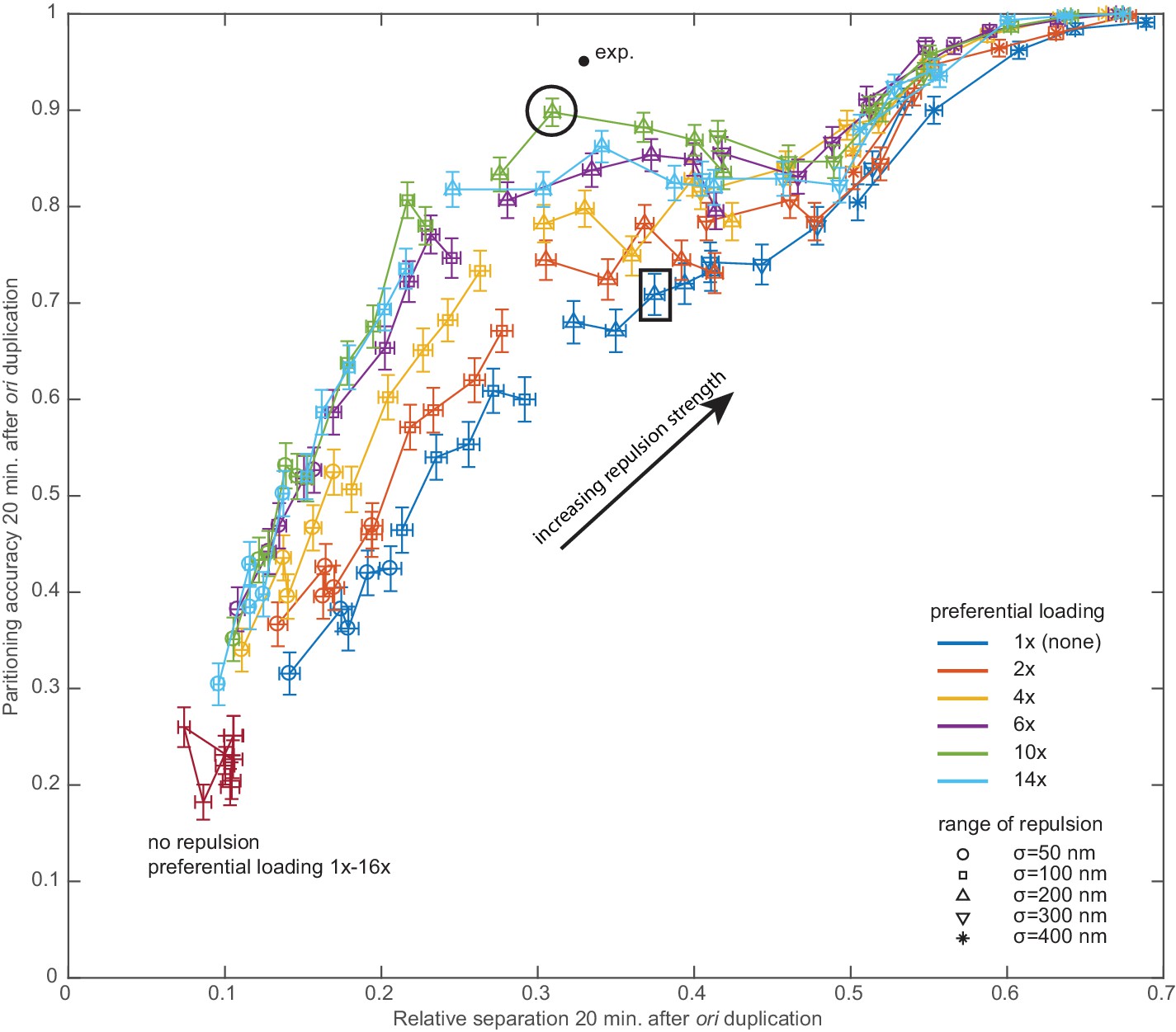
Results from a parameter sweep over the two properties specifying the repulsion, its range (symbols) and its strength (increasing as indicated). Different colours indicate different levels of preferential loading (1x-14x). The dark red points are from simulations without repulsion, with only the preferential loading varying. Each data point is the mean over 450 independent simulations (performed as in Figure 4—figure supplement 1). The output is the partitioning accuracy and relative separation measured 20 min. after ori duplication (which varies stochastically). Error bars are standard errors. The experimental data point is from an analysis of the data of Kuwada et al. (2013) (see also Figure 4f). The black circle indicates the simulations subsequently shown and analysed in Figure 4. The black rectangle indicates the simulations shown in Figure 4—figure supplement 3.
Figure 4—figure supplement 3
Repulsion between ori alone results in incorrect dynamics.
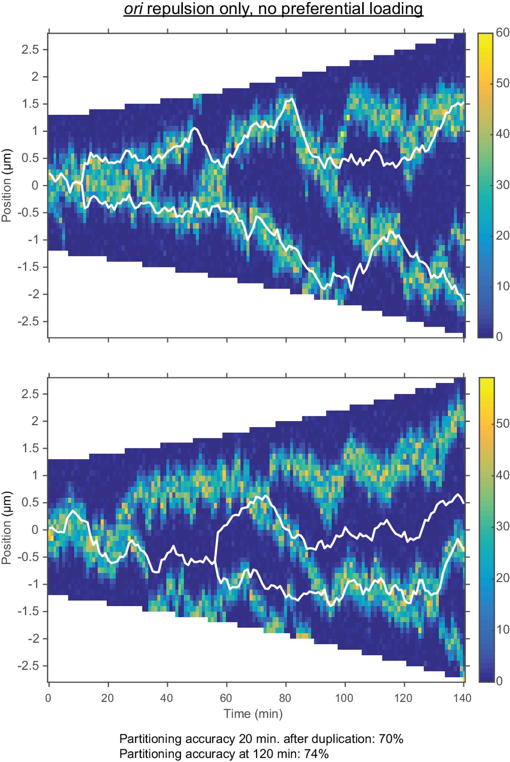
Two representative kymographs of the number of MukBEF molecules and ori positions during exponential group (doubling time 120 min.) with repulsion between ori but without preferential loading. The colour scale represents the number of MukBEF molecules; white lines show the positions of ori. The range of the repulsive force is 200 nm and indicted by the rectangle in Figure 4—figure supplement 2.
Figure 5 with 2 supplements
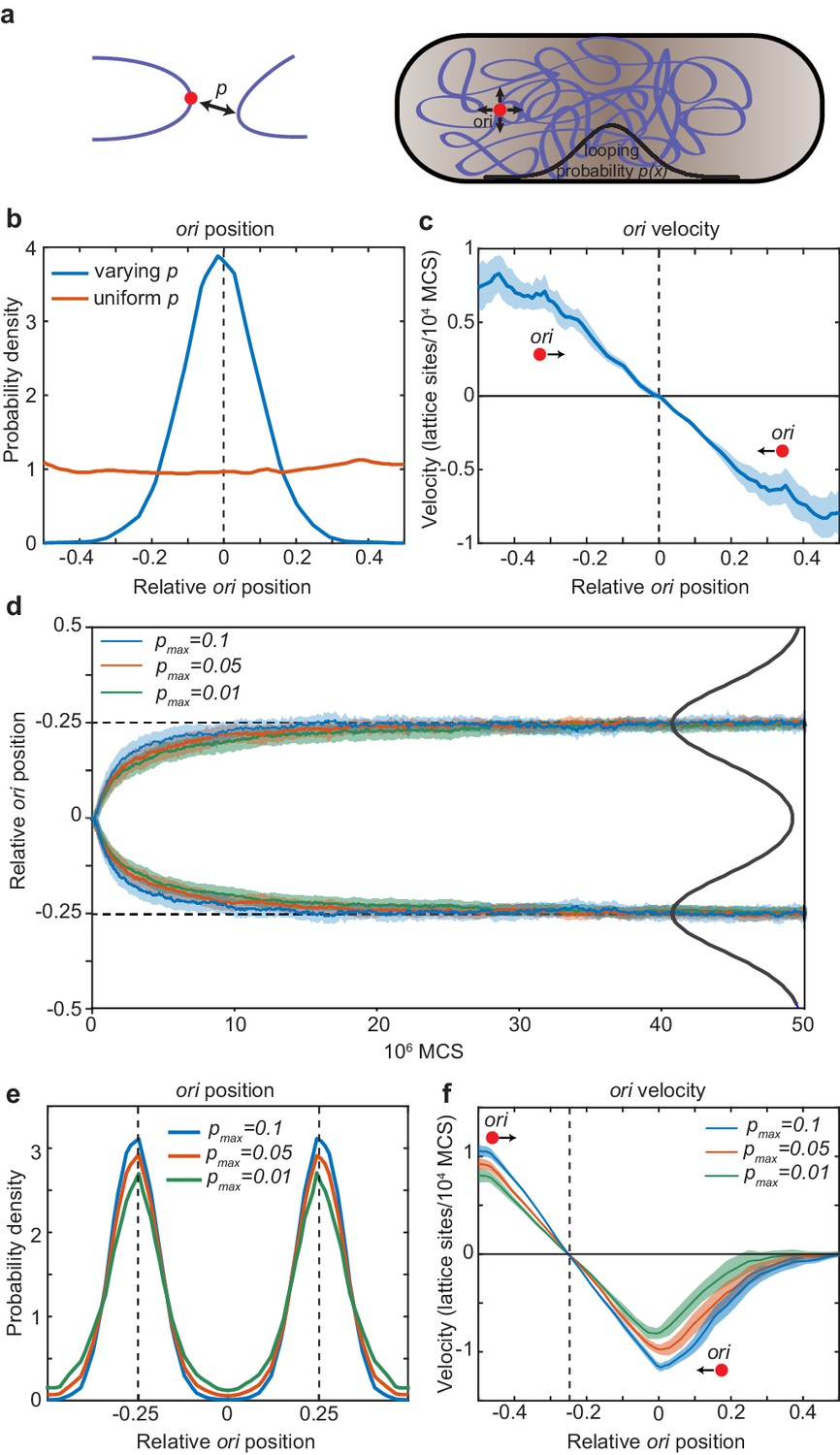
Directed movement of ori can arise from spatially-dependent looping interactions.
(a) A diagram illustrating how the elastic fluctuations of ori allow it sample the spatial looping probability distribution. It is therefore more likely to form a loop with a locus that is closer to mid-cell, where the probability of looping, p, is higher. (b) Probability density of relative ori position along the long axis of the cuboid (aspect ratio 4:1) with (blue) and without (red) a spatially-varying looping probability (a Gaussian shaped distribution centred at 0 with standard deviation 0.1 in units of long-axis length; the looping probabilty at 0, pmax, is 0.02.). See also Figure 5—figure supplement 1. (c) The mean ori velocity along the long axis as a function of relative position. Shaded area indicates standard error. In (b) and (c), the ori position was read out every 50000 Monte Carlo time-steps (MCS) and data is from 50 independent simulations with approximately 10000 data points from each. (d) The mean relative position of oris along the long axis of the cuboid during segregation. Simulations were initialized with two overlapping polymers with the ori monomers at the middle position. We used a looping probability distribution (black line) with the shape of the sum of two Gaussians centred at the quarter positions with standard deviation 0.1 in units of long-axis length. Results for different values of the looping probability at the quarter positions, pmax, are shown. Data is from 500 independent simulations read out as in (c). Shading indicates the standard error. (e) Probability density of relative ori positions in simulations of two polymers described in (d) after equilibration i.e. the polymers have segregated to opposite ends of the cuboid. (f) The mean step-wise ori velocity for one of the two segregated polymers. This polymer is confined to the left side of the cuboid. The ori experiences a restoring velocity to the approximate −1/4 position. The right half of the curve is due to infrequent excursions of the ori into the other half of the cuboid. The shaded region indicates standard error. See also Figure 5—figure supplement 2.
Figure 5—figure supplement 1
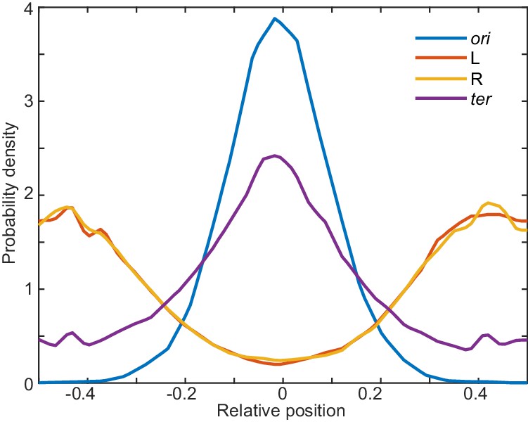
Positions of other loci.
Probability density of relative ori (0°), L (−90°), R (+90°), and ter (180°) position along the long axis of the cuboid in the presence of a spatially-varying probability for ori to forms loops as in Figure 5b. L and R are generally positioned at the ends of the cuboid, while the ter is positioned roughly a mid-cell, though with a substantially broader distribution than ori. Data is from 50 independent simulations. Results are consistent with the histograms (from a single simulation) of Junier et al. (2014), in which the ori is localised to mid-cell by an imposed strong harmonic potential.
Figure 5—figure supplement 2
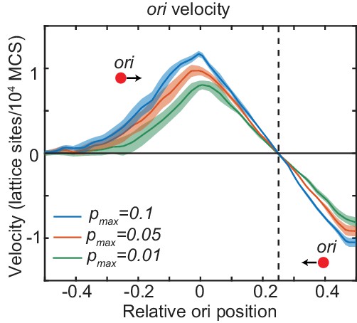
The mean ori velocity for the polymer not shown in Figure 5f.
This polymer is confined to the right side of the cuboid and its ori experiences a restoring velocity to the approximate +1/4 position. Otherwise as in Figure 5f.
Figure 6 with 1 supplement
Preferential loading and entropic repulsion together lead to the observed ori dynamics.
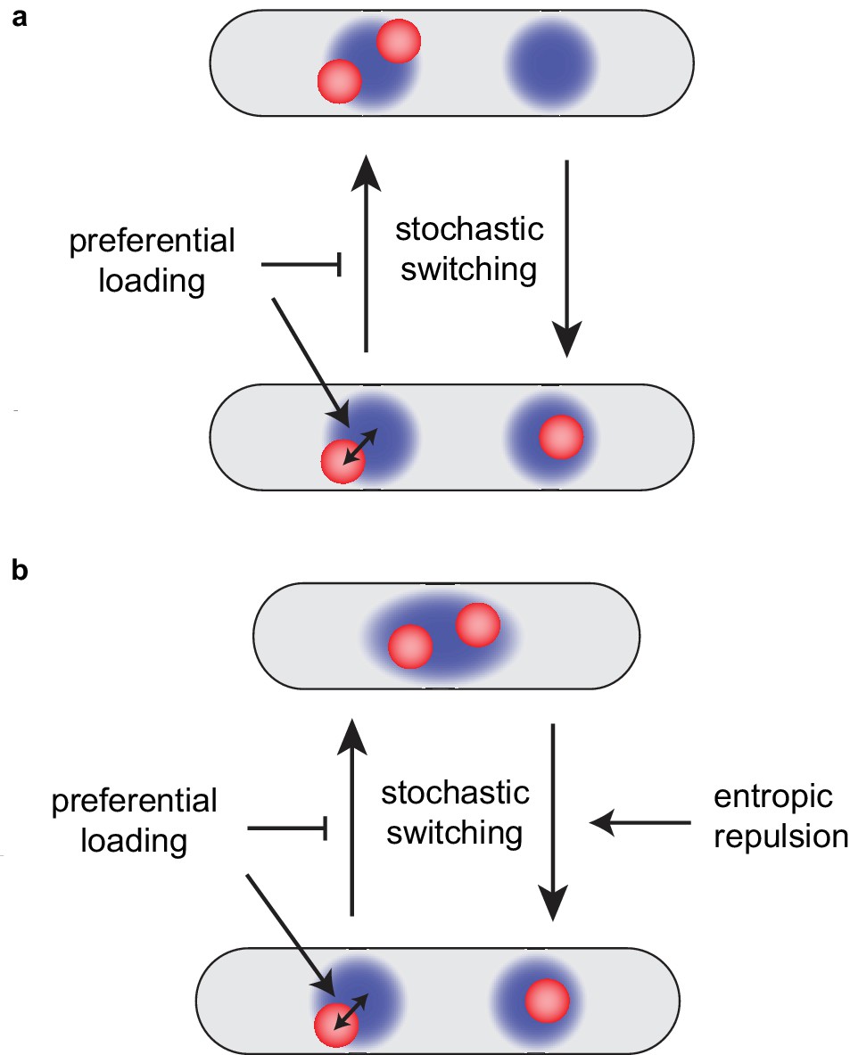
(a) Schematic illustrating the effect of preferential loading of MukBEF at ori in the simulations of non-growing cells. In the presence of preferential loading ori (red) and MukBEF foci (blue) are strongly associated with both each other and the quarter positions. This acts to stabilise the desirable correctly partitioned configuration (bottom) over the un-partitioned one (top). In the absence of preferential loading, both configurations have equal stability (are equally likely). See also Figure 6—figure supplement 1. (b) Short-range entropic repulsion promotes the timely separation of newly duplicated ori. Their separation promotes splitting of MukBEF foci. MukBEF-ori then move together to opposite quarter positions with preferential loading promoting their association and the stability of the quarter-positioned configuration.
Figure 6—figure supplement 1
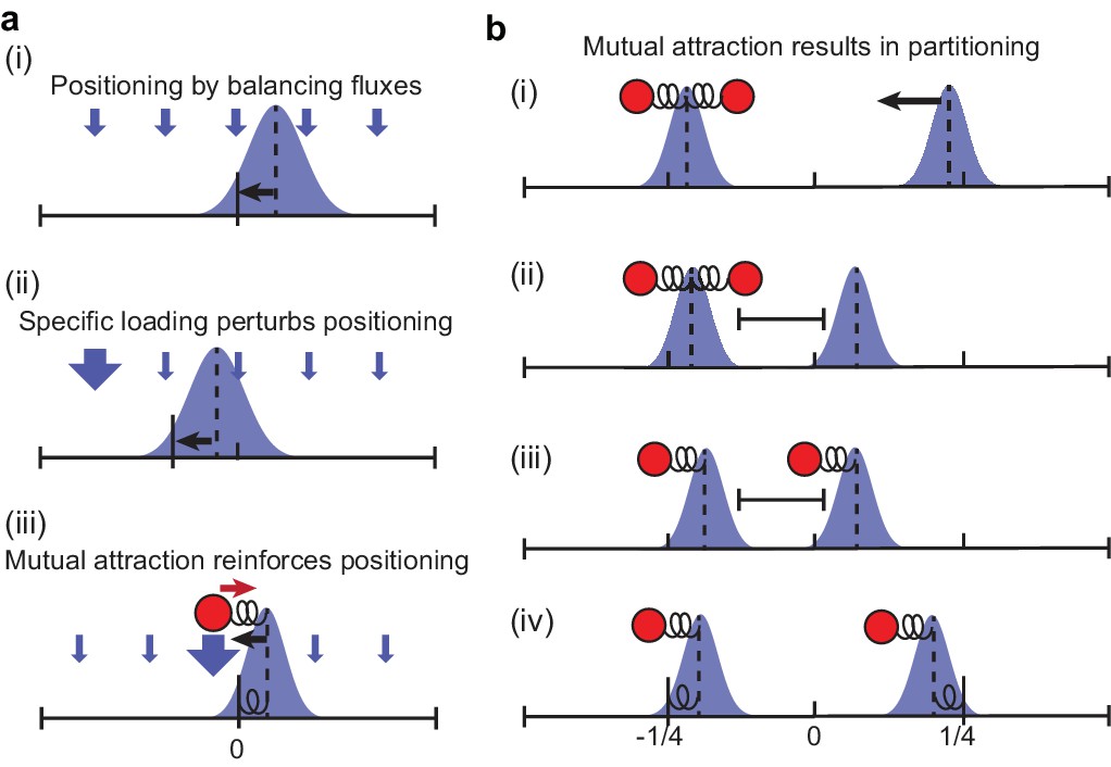
Schematic of how preferential loading leads to partitioning.
(a) MukBEF self-organises via a Turing instability into regions of high local density (foci). The position of these foci is determined by the balancing of fluxes originating from the well-mixed cytosolic state. With spatially homogeneous loading of the well-mixed state onto the nucleoid, the fluxes balance, in the case of a single focus, at the mid-cell position (i). An object (the ori) that is attracted up the resulting gradient will also be positioned at mid-cell. However, if loading is not homogeneous, then the position at which the fluxes balance changes (ii). If higher loading occurs at the ori, then the mutual attraction between the self-organised MukBEF focus and the ori results in the suppression of fluctuations, strong colocalisation and positioning at mid-cell (iii). The system is analogous to a compound spring with the fixed end at mid-cell (but with a non-trivial relationship between the spring constants and preferential loading ratio). At high levels of preferential loading, colocalised MukBEF-ori becomes less sensitive to the (decreased) incoming flux from other regions, and is therefore less attracted towards mid-cell, resulting in more diffusive behaviour and a broader position distribution. (b) Suppose both ori have been pulled towards the same MukBEF focus. Due to the flux imbalance, the MukBEF focus without an ori will be effectively pulled towards the other one (i) until the fluxes balance (ii). The stochastic nature of ori and MukBEF movement means that at some point one ori leaves the influence of its MukBEF focus and becomes associated to the other focus (iii). This is aided by the fact that the two MukBEF foci repulse each other so that the first MukBEF focus is prevented from following the ori. After the ori associates to the other MukBEF focus, the balance of fluxes is again disturbed and MukBEF-ori move as single units towards opposite quarter positions (iv). Due the strong association and reduced spatial fluctuations caused by preferential loading, this is the stable configuration and the system does not revert back to (i). See also Figure 6.
Figure 7 with 1 supplement
The model qualitatively reproduces the observed ori dynamics during multi-fork replication.
An example kymograph showing multi-fork replication. See also Figure 7—figure supplement 1. Results qualitatively agree with Youngren et al. (2014). All parameters are as in Figure 4, except for the total number of MukBEF molecules, which was increased from 520 nM to 1000 nM, broadly in line with previous measurements (Li et al., 2014).
Figure 7—figure supplement 1
Histograms of ori positions during multi-fork replication.
(a) Histogram of relative ori positions at time points at which there are two ori. (b) Histogram of relative ori positions at time points at which there are four ori. Results are from 450 independent simulations performed as in Figure 7.
Tables
Table 1
Common Parameters.
https://doi.org/10.7554/eLife.46564.024| Parameter | Value |
|---|---|
| α | 0.5 s−1 |
| β | 1.5 × 10⁻⁴ nM−2 s−1 |
| γ | 3.6 s−1 |
| δ | log(2)/50 s−1 |
| ϵ | 3δ |
| Du | 0.3 µm2 s−1 |
| Dv | 0.012 µm2 s−1 |
| V (volume at length 2.5 µm) | 1.25 × 10⁻¹⁵ L |
| C | 520 nM |
Table 2
Additional parameters used in Figure 2d, Figure 2—figure supplements 1–4, Figure 3, Figure 3—figure supplement 1.
Obtained by fitting the model without preferential loading to the data of Kuwada et al. Some simulations use preferential loading as stated in the legend or on the plot axis.
| Parameter | Value |
|---|---|
| 5.4 × 10⁻⁵ µm2 s−1 | |
| 0.026 µm |
Table 3
Additional parameters used in Figure 2e,f, Figure 4, Figure 4—figure supplement 1–3.
Obtained by fitting the model with 6X preferential loading to the data of Kuwada et al. (Figure 2e,f).
| Parameter | Value |
|---|---|
| 5.1 × 10⁻⁵ µm2 s−1 | |
| 0.052 µm |
Table 4
Additional parameters (together with those in Table 3) used in Figure 4—figure supplement 3.
ori repulsion without preferential loading.
| Parameter | Value |
|---|---|
| 5 s−1 | |
| 200 nm |
Table 5
Additional parameters (together with those in Table 3) used in Figure 4.
ori repulsion with 10x preferential loading.
| Parameter | Value |
|---|---|
| 1 s−1 | |
| 200 nm |
Additional files
-
Transparent reporting form
- https://doi.org/10.7554/eLife.46564.029
Download links
A two-part list of links to download the article, or parts of the article, in various formats.
Downloads (link to download the article as PDF)
Open citations (links to open the citations from this article in various online reference manager services)
Cite this article (links to download the citations from this article in formats compatible with various reference manager tools)
Self-organised segregation of bacterial chromosomal origins
eLife 8:e46564.
https://doi.org/10.7554/eLife.46564


