Figures and data in Population adaptation in efficient balanced networks | eLife

Figures
Additional files

8 figures and 1 additional file

Figures

Figure 1

Download asset Open asset

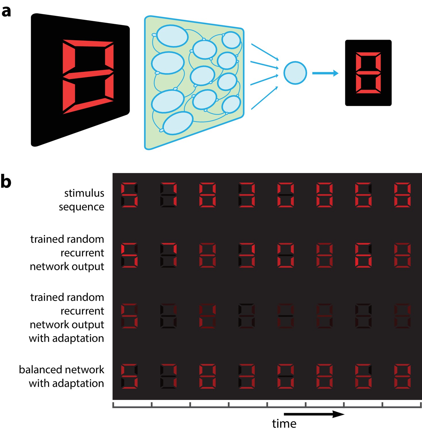
Digital number encoding network.

(a) Schematic of a 7-dimensional input (one dimension for each bar position of a digital interface) being presented to a random recurrent network that sends input to a readout layer (here represented by a single neuron). (b) Top, a sequence of digits that serve as stimuli (presented for 200 ms each, spaced by 100 ms between digits). Second row, decoded output of random recurrent network with optimal decoder (trained on 100 samples of completely random patterns). Third row, decoded output of same random recurrent network as above but with adapting neuron responses. Bottom row, balanced network with adaptation derived from efficient coding framework. [All rows: 400 neurons, $τ = 5 m s$ for neural responses integrated by decoder; 3rd and 4th row: $μ = 0.02; τ_{a} = 2000 m s$ for the adaptive firing rates].

https://doi.org/10.7554/eLife.46926.003

Figure 2

Download asset Open asset

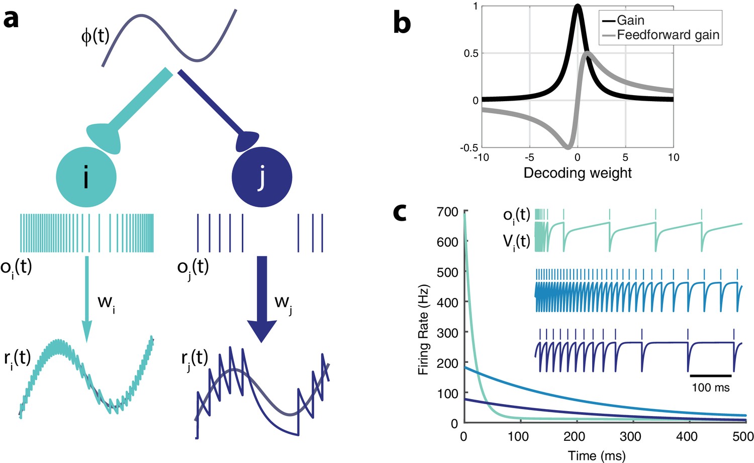
Intrinsic model neuron properties.

(a) High gain neurons (light blue) are intrinsically excitable and due to their small decoding weights they are precise while low gain neurons (dark blue) are less excitable and less precise. An arbitrary input, $ϕ (t)$ , elicits distinct responses from the two neurons (spikes train $o_{i}$ and $o_{j}$ , respectively). Neurons send a filtered response, $r_{i}$ , $r_{j}$ , to the decoder weighted by $w_{i}$ and $w_{j}$ , respectively. (b) Relationship between gain $g_{i} = 1 / (w_{i}^{2} + μ)$ , feedforward gain $g_{i} w_{i} = w_{i} / (w_{i}^{2} + μ)$ , and decoding weight $w_{i}$ ( $μ = 1$ ). (c) Different gains give neurons distinct adaptation dynamics. Instantaneous spiking rates in response to a constant input are plotted over time for three model neurons with different decoding weights (light blue, w = 1; medium blue, w = 5; dark blue, w = 9). High gain neurons have the steepest adaptation (light blue) whereas low gain neurons (dark blue) do not adapt as rapidly given the same input. Inset shows the voltage trace, $V (t)$ , and spike train, $o (t)$ , for each example neuron.

https://doi.org/10.7554/eLife.46926.004

Figure 3

Download asset Open asset

Two-neuron network.

(a) Schematic of recurrently connected two-neuron network derived from efficient coding framework. Neuron 1 is strongly excitable ( $w_{i} = 1$ ), while neuron 2 is weakly excitable ( $w_{i} = 2$ ). (b) Spikes from neuron 1 (light blue) and neuron 2 (dark blue) show the transient response of the strongly excitable neuron and the delayed, but sustained response of the weakly excitable neuron (top) in response to a constant stimulus. Postsynaptic activity, $r (t)$ (bottom) [ $μ = 0.02, τ = 25 m s, τ_{a} = 1000 m s, ϕ (t) = 10$ ]. (c) The balanced network with adaptation follows a linear manifold (left), whereas the network without recurrent connections but with adaptation cannot be linearly decoded (right). (d) The cost ( $μ \sum_{n} f_{n}^{2}$ , yellow) accumulates steeply until neuron one adapts and neuron two is recruited and the cost increases at a slower rate. The network representation (orange) is maintained despite the redistribution of activity among the neurons.

https://doi.org/10.7554/eLife.46926.005

Figure 4

Download asset Open asset

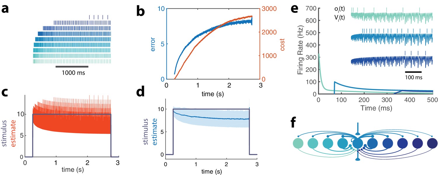
Adapting population of heterogeneous neurons.

(a) Spike raster of all 10 neurons in a balanced network with adaptation in response to a pulse stimulus ( $μ = 0.2, τ = 5, τ_{a} = 1000, ϕ (t) = 10, 𝒘 = [1, 2, \dots, 10]$ ). Neurons are ordered from weakly excitable (top, dark blue) to highly excitable (bottom, light blue). (b) Both the error ( ${(ϕ (t) - \hat{ϕ} (t))}^{2}$ , blue) and cost ( $μ \sum_{n} f_{n}^{2}$ , orange) accumulate over time. (c) The network estimate ( $\hat{ϕ} (t)$ , orange) tracks the stimulus ( $ϕ (t)$ , gray) with increasing variance. (d) The smoothed network estimate (blue line) shows a biased estimate with increasing variance (blue shade, standard deviation). (e) Instantaneous spiking rates of 3 example neurons in the network. Inset shows the voltage trace, $V (t)$ , and spike train, $o (t)$ , for each example neuron. (f) Schematic of 10-neuron balanced network showing only connections to and from the middle neuron. Excitatory connections are shown as triangles and in this particular network are only found in the feedforward and output connections. Inhibitory connections are shown with small circles and make up only the recurrent connections.

https://doi.org/10.7554/eLife.46926.006

Figure 5

Download asset Open asset

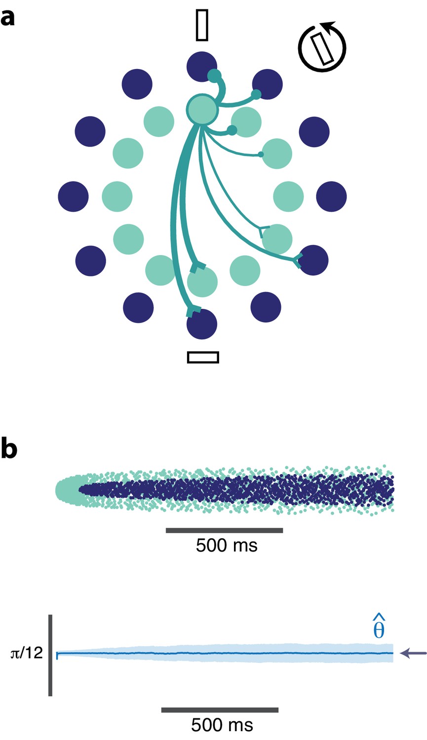
Orientation coding-network.

(a) Schematic showing the dual-ring structure of the network of high gain (light blue) and low gain (dark blue) neurons. Some of the recurrent connections from the outlined light blue neuron are illustrated to show that a neuron inhibits its neighbors most strongly and excites neurons with opposing preferences (inhibitory connections are shown as circles, excitatory connections are shown as chevrons). (b) Spike raster (top) of population activity showing the evolution of the population response during a prolonged stimulus presentation of a constant orientation. Rasters are displayed in order of neuron orientation preferences. The decoded orientation is steady while the variance increases over time (bottom). Arrow indicates the stimulus orientation. ( $μ = 0.1, τ = 5 m s, τ_{a} = 2000 m s$ , $η = 10$ , stimulus magnitude C = 50, 200 neurons).

https://doi.org/10.7554/eLife.46926.007

Figure 6

Download asset Open asset

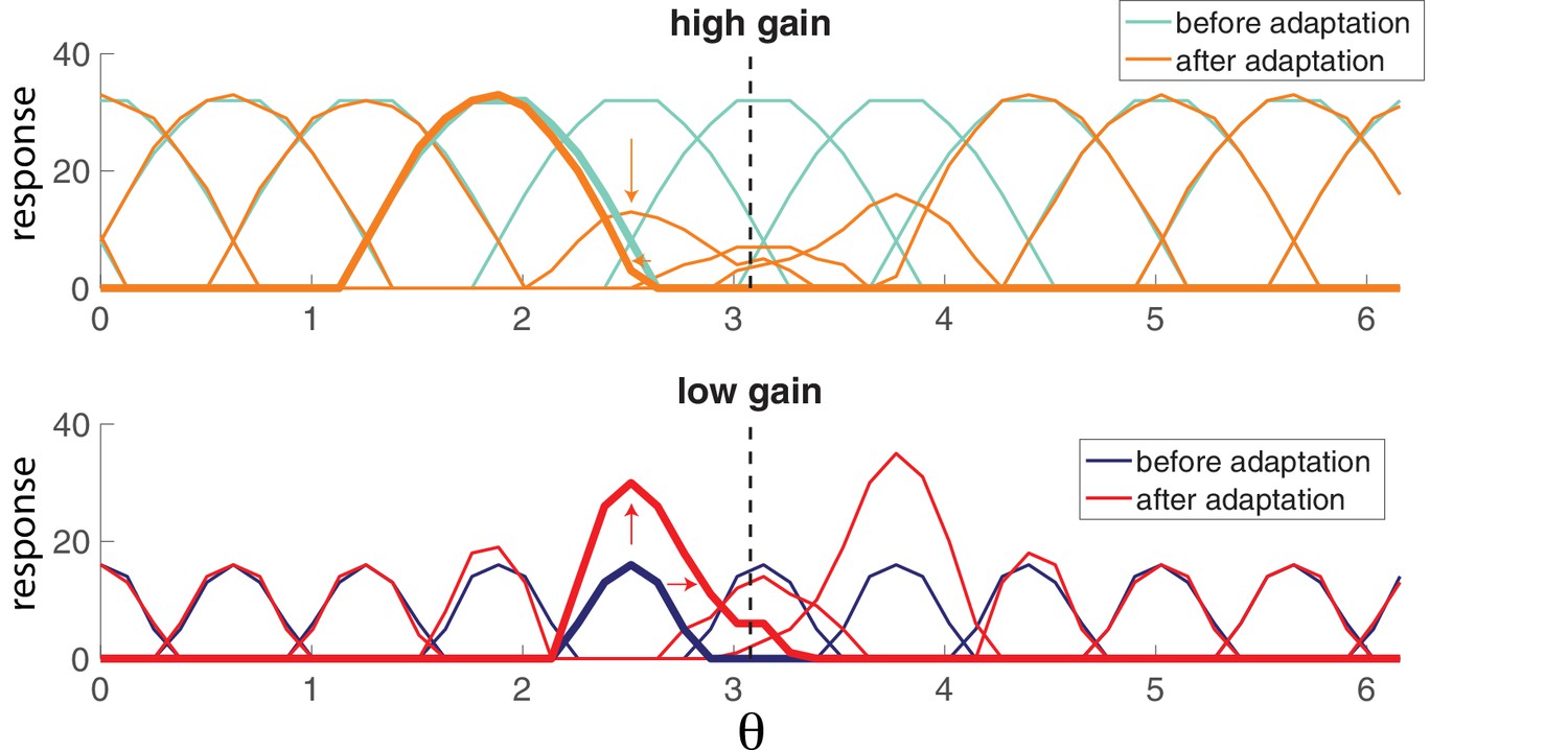
Population adaptation tuning curves show neuron responses to a full range of test orientations (x-axis) after adaptation to a single orientation (black dashed line).

Top, tuning curves for strongly excitable neurons before adaptation (light blue) are broad. After adaptation (orange), tuning curves near the adaptor are suppressed. Bottom, tuning curves for weakly excitable neurons before adaptation (dark blue) show less activation than for high gain neurons and more specific tuning. After adaptation (red), flanking curves are facilitated and shifted toward adaptor. [ $μ = 0.1, τ = 5 m s, τ_{a} = 2000 m s$ , $η = 10$ , stimulus magnitude C = 50, 200 neurons].

https://doi.org/10.7554/eLife.46926.008

Figure 7

Download asset Open asset

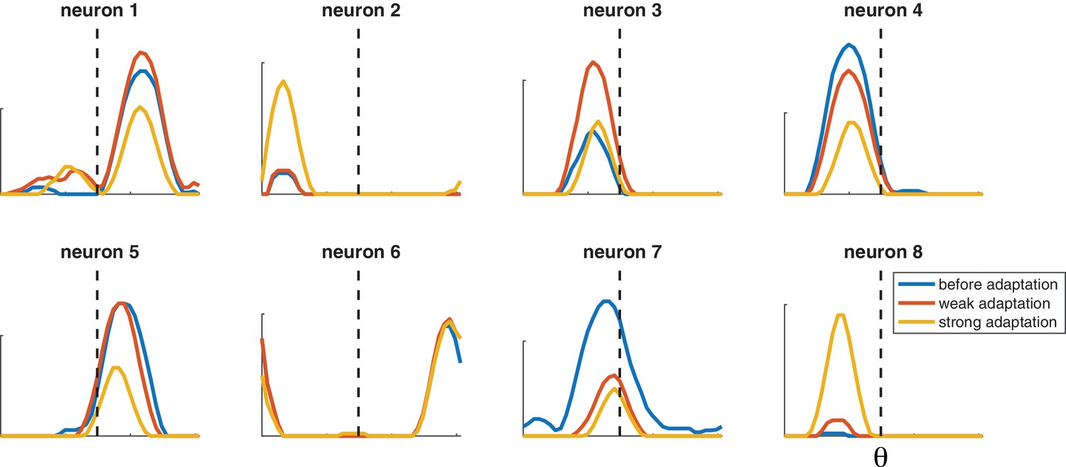
Selected tuning curves from orientation network with random decoder weights (and thus random neuron gains).

Blue curves, before adaptation; red curves, after weak adaptation; yellow curves, after strong adaptation. Some neuron responses are suppressed after adaptation while others are facilitated, and some tuning curves shift laterally after adaptation. Dashed lines indicate adaptor orientation. [ $μ = 0.2, τ = 5 m s, τ_{a} = 1000 m s, η = 1$ , weak stimulus magnitude C = 10, strong stimulus magnitude C = 50, test stimulus magnitude C = 10, 200 neurons].

https://doi.org/10.7554/eLife.46926.009

Figure 8

Download asset Open asset

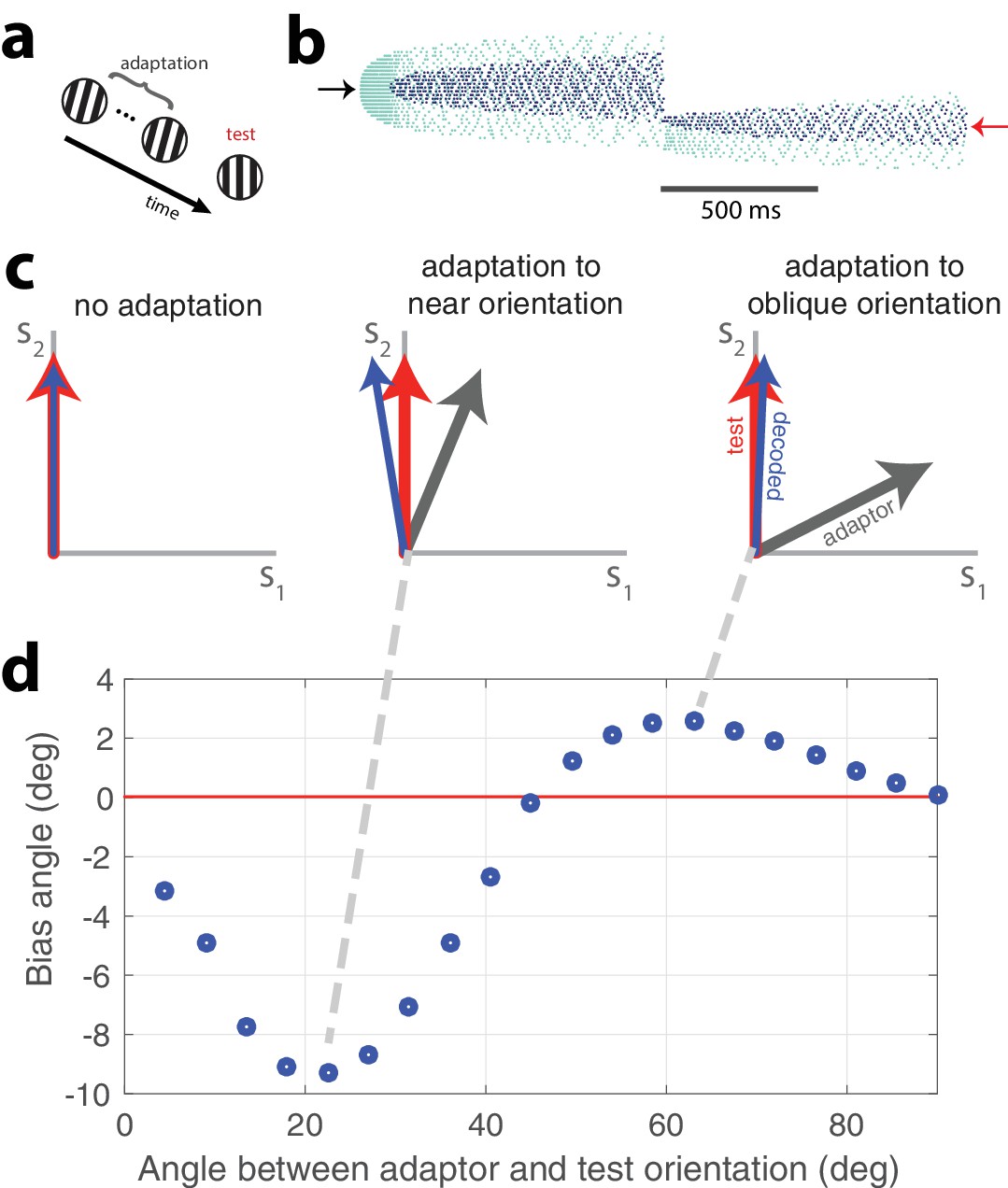
Tilt illusion.

(a) Schematic of tilt adaptation protocol. (b) Network activity in response to an adapting stimulus followed by a test stimulus. Rasters are ordered by neurons’ orientation preferences. Black arrow, neurons that prefer adapting orientation; red arrow, neurons that prefer test orientation ( $μ = 0.1, τ = 5 m s, τ_{a} = 2000 m s, η = 10$ , 200 neurons, adaptor C = 50, test C = 25). (c) Examples of tilt bias: (left) no bias before adaptation, (middle) network estimate is biased away from test stimulus and adaptor when adaptor is near test orientation, (right) estimate is biased towards adaptor when adaptor is at large angle to test stimulus (red arrow, test orientation; grey arrow, adaptor; blue arrow, decoded orientation to test orientation after adaptation). (d) Estimate bias is repulsive for near adaptation and attractive for oblique adaptation. Adaptor is presented for 2 s and test orientation is presented for 250 ms ( $η = 0$ , adaptor C = 25, test C = 5).

https://doi.org/10.7554/eLife.46926.010

Additional files

Transparent reporting form: https://doi.org/10.7554/eLife.46926.011
Download elife-46926-transrepform-v1.docx

Download links

A two-part list of links to download the article, or parts of the article, in various formats.

Downloads (link to download the article as PDF)

Article PDF

Open citations (links to open the citations from this article in various online reference manager services)

Mendeley

Cite this article (links to download the citations from this article in formats compatible with various reference manager tools)

Gabrielle J Gutierrez
Sophie Denève

(2019)

Population adaptation in efficient balanced networks

eLife 8:e46926.

https://doi.org/10.7554/eLife.46926

Sign up for email alerts

Privacy notice