Layer 6 ensembles can selectively regulate the behavioral impact and layer-specific representation of sensory deviants
- Department of Neuroscience and Carney Institute for Brain Science, Brown University, United States
- Department of Brain and Cognitive Sciences, MIT, United States
Figures
Figure 1 with 1 supplement

In a natural behavior, strong optogenetic drive of L6 causes a sensory deficit.
(a) To test the impact of L6 modulation in a naturalistic context, we used an unrestrained Gap Crossing task and applied high or low power optogenetic drive to L6 CT cells (ChR2 in NTSR-1 cre line). (b) Example trace (nose position over the gap) where strong optogenetic L6 drive disrupted Gap Crossing behavior, causing the mouse to retreat before crossing. (c) Strong L6 drive made mice less likely to cross the gap (N = 514 trials, bootstrapped 95% confidence intervals (CIs)). (d) In contrast, weaker L6 drive did not reduce crossing probability (N = 751 trials) but led to a small increase in crossing probability.
Figure 1—figure supplement 1

Overview of trial structure and timing for the experimental paradigms used in this study.
(a) Experimental preparation for head-fixed detection behavior (Figure 3, N=4 mice). Mice were head-posted and rested on a platform. Correct stimulus detection was rewarded with water. (b) Trial timing for head-fixed behavioral testing. Early licking in a variable timeout period reset the timeout. (c) State diagram for head-fixed detection task. (d) Setup for unrestrained gap-crossing behavior (Figure 1, N=6 mice). Mice freely crossed between two platforms for water reward. The platform distances were chosen randomly between 4-6cm, and on a subset of trials the target platform was pulled back by ~2mm mid-exploration. (e) Timing structure for gap-crossing. All events except for the timing of the laser stimulus and the gap-repositioning were chosen freely by the animals. (f) State diagram for gap-crossing. (g) Setup for chronic electrophysiology (Figures 4, 6, 7, 9, N=5 mice). Correct stimulus detection was rewarded with water. Mice rested or walked/ran on a spherical treadmill to promote comfort and longer recording sessions. (h) Trial timing for electrophysiology. No timeout periods or catch trials were used. (i) Setup for 2-photon imaging (Figure 5,8,9, N=2 mice) and simultaneous 2-photon imaging and optogenetics (Figure 5,9, N=4 mice). Mice were not water restricted and rested or walked/ran on a spherical treadmill. (j) Trial timing for imaging experiments. No reward was used, but stimulus timing was randomized as in other conditions.
Figure 2 with 2 supplements
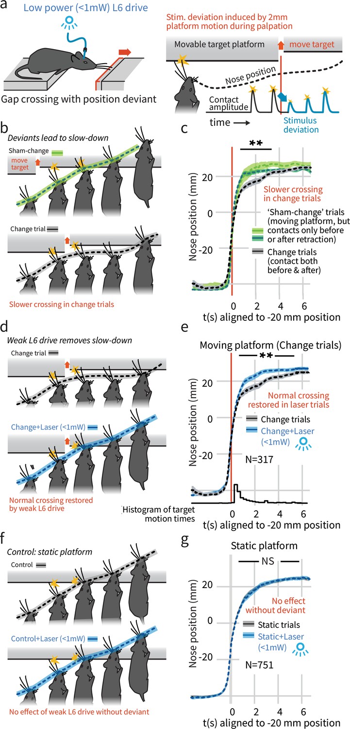
In a natural behavior, weak L6 drive selectively negates processing of deviant stimuli.
(a) To create a sudden, small sensory deviation, in the Gap Crossing with Deviation task the target platform was retracted by ~2 mm during bouts of tactile sampling. Prior high-speed videography studies have shown this small, unexpected deviation in the position of the platform leads to changes in vibrissal motion, including reduced deflection amplitudes (Figure 9 of Voigts et al., 2015). (b) When the platform was retracted in the middle of a bout of vibrissal contacts (black trace), mice slowed their approach relative to control trials where they contacted the target either exclusively before (light green) or after (dark green) platform retraction. (c) Summary statistics (95% CIs) of mouse position over time in the three trial types. (d) Weak L6 drive removed the deceleration associated with platform position deviants. (e) During weak L6 drive, the time course of the Gap Crossing with Deviation task does not show the signature deceleration created by a change in platform position during palpation. (f, g) Weak L6 drive had no effect on the Gap Crossing when the platform was static, showing that it selectively abolished the reaction to platform position deviants with little effect on other sensory and sensorimotor function. See Figure 2—figure supplement 2 for per-mouse data.
-
Figure 2—source data 1
Gap crossing speed across sham-change, control, and L6 drive conditions.
- https://cdn.elifesciences.org/articles/48957/elife-48957-fig2-data1-v2.zip
Figure 2—figure supplement 1
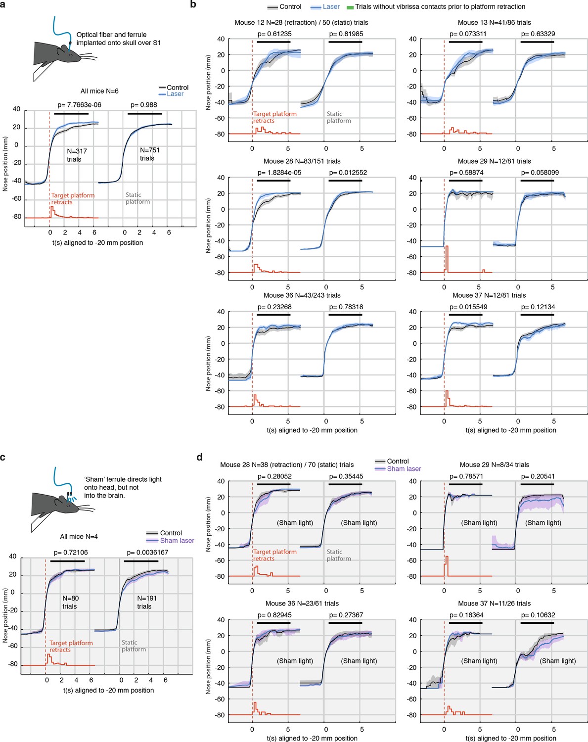
Per-mouse analysis of freely behaving gap-crossing and sham-laser control experiment.
(a) Summary statistics for gap-crossing in the low-power (<1 mW laser) condition, same as Figure 1 Left: Trials with retracting target (retraction times indicated in red, sum-normalized histogram). Right: return trials (opposite direction) with a static target platform. P-values are from a rank sum test using the mean position for each trial in the region indicated with a black line. Only trials where vibrissae overlap the platform before and after the platform retraction were included because only these trials present sensory change to the mouse. This analysis was performed using fully automated vibrissa tracking and no explicit collision detection other than intersection of vibrissae and target edge was used. (b) Analysis for the gap-crossing experiment for each individual animal. (c) Same as panel a, but for sham-laser condition. Mice (N = 4) were tested as usual, but a 'sham' ferrule directed the laser light diffusely over the entire head of the animal instead of coupling it into the implanted ferrule. These control experiments were run with higher laser powers of ~10 mW to ensure that the light was always brighter and more visible to the animals than in the main experiment. (d) Analysis for the sham-laser experiment for each individual animal. There was no specific effect on stimulus change detection.
Figure 2—figure supplement 2
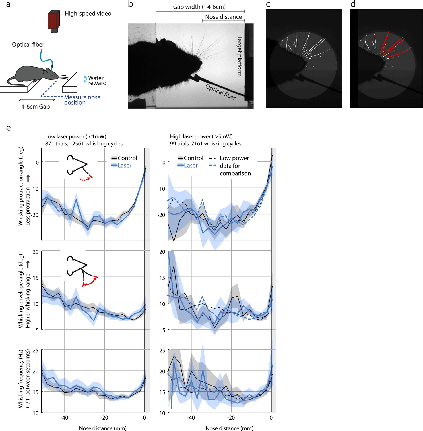
Whisking pattern kinematics in the gap-crossing task are not impacted by laser stimulation.
Neither the low-power (<1 mW) nor the high-power (>5 mW) optogenetic L6 CT drive caused significant disruption of the sensorimotor whisking pattern in the gap-crossing task. (a) Overview of setup for gap-crossing (Chater et al., 2006; Rao and Ballard, 1999; Courchesne et al., 1975; Tiitinen et al., 1994). (b) Example raw image from gap-crossing experiment. (c) Output of the convolutional neural network / vibrissa-identification stage of the vibrissa tracker (github.com/jvoigts/whisker_tracking). (d) Same as panel (c) but individual vibrissa segments are identified with a Hough transform. (e) Vibrissa kinematics, resolved by nose-target platform distance (N = 4 mice with vibrissa tracking, 970 trials total) for the low-power (<1mW ChR2 drive) and high power (>5mW) conditions. All plots are median and 95% confidence bounds for the median via bootstrapping. The low-power medians (left) are re-plotted as dotted lines in the high power condition (right). Top row: maximum protracted angle per vibrissa protraction cycle. Values closer to 0 correspond to smaller vibrissal protractions. Middle: Whisking pattern envelope amplitude (Hilbert-transform on 8-20 Hz filtered median whisker angle). Bottom: Whisking frequency computed from time between whisking pro/retraction setpoints. Data points above 30 Hz were excluded.
-
Figure 2—figure supplement 2—source data 1
Whisking dynamics for the Gap rossing task.
- https://cdn.elifesciences.org/articles/48957/elife-48957-fig2-figsupp2-data1-v2.zip
Figure 3 with 2 supplements
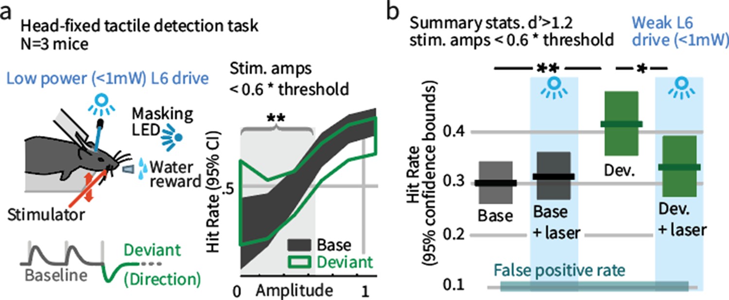
Weak L6 drive negates the improved sensitivity driven by inclusion of deviant stimuli in a head-fixed detection task.
(a) Left: Mice were trained on a go/no-go stimulus detection task. Mice were not explicitly trained to report the presence of a deviant. In 50% of trials, direction deviants were present at positions 2–4 in the stimulus train. Right: Example psychometric curve from one mouse. Deviants increased detection rates for weak stimuli that were less than 60% of the threshold amplitude (gray region). (b) Box plots show 95% CIs (via bootstrap) for the detection probabilities for this range of stimuli from three mice for baseline and deviant-containing stimuli, for the control (blue masking light) and laser (weak L6 drive, <1 mW) condition.
Figure 3—figure supplement 1
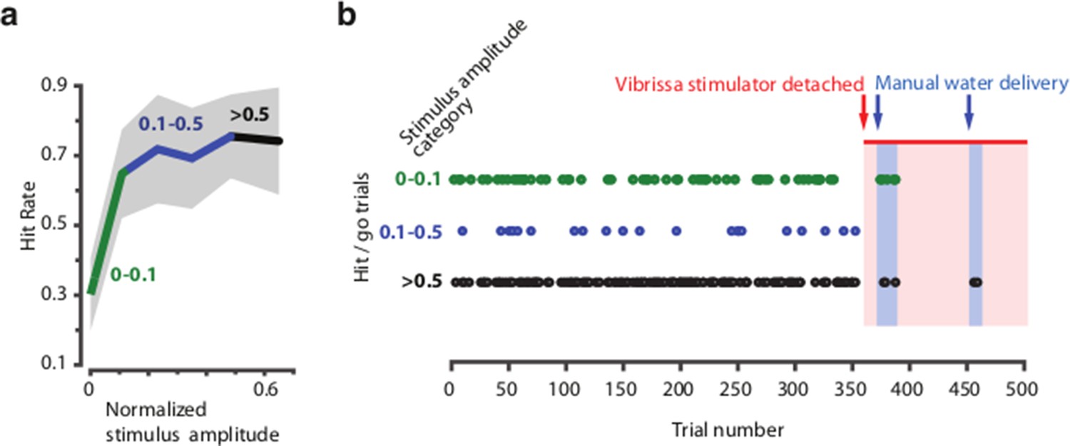
Head-fixed behavior depends on vibrissa stimulation and is independent of other (auditory or visual) cues.
Mice were trained to detect vibrissa stimulation (in a separate experiment) using the same vibrissa stimulator, masking noise, absence of <650nm light, and behavioral protocol as described in Methods. (a) Psychometric curve for one session, stimulus amplitudes were split into three categories based on stimulus amplitude (<0.1, 0.1 – 0.5 and >0.5 x maximum amplitude). (b) Raster plot of successful detections (licks in go-trials) over the session (500 trials). Misses or catch trials are not plotted. Towards the end of the session, the stimulator was opened freeing the vibrissae, but remained in the same position, so that vibrissa contact to the stimulator was still possible and any vibration, visual or auditory cues were the same as in the beginning of the session. In two blocks, reward was given manually to verify that the animal was still attentive and could react to reward delivery (indicated by the click of a solenoid) with licking (indicated as hits in cases where water was given in non-catch/go trials).
Figure 3—figure supplement 2
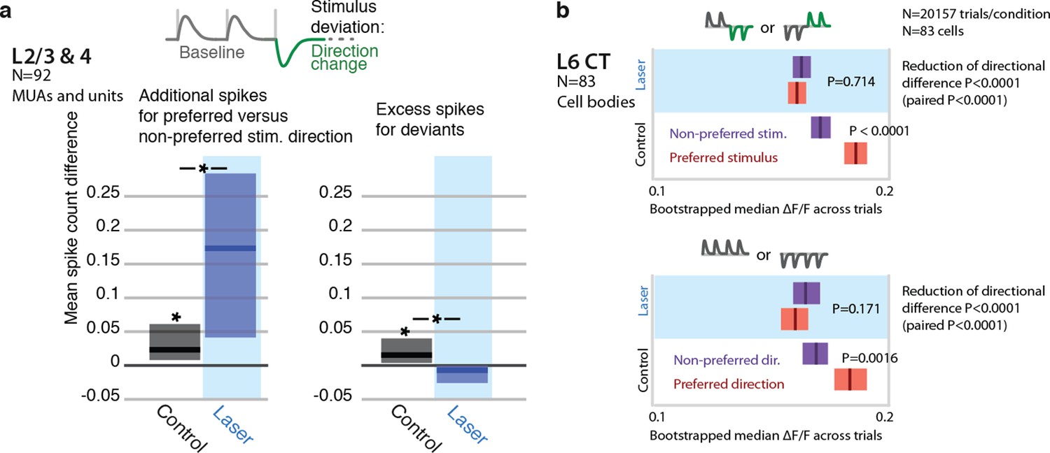
Encoding of directional deviants, and effect of L6 activation.
The direction changes employed for the head-fixed detection task differ from the amplitude deviants used throughout the rest of the study. We therefore also examined the impact of weak L6 CT drive on the neural representation of direction deviations in separate recordings. In L6 CT (GCaMP6s imaging, N = 83 sensory responsive neurons), encoding of stimulus direction was disrupted by weak optogenetic drive (P<0.05, baseline direction and direction changes). Similarly, L2/3 and L4 neurons (N=92 units and MUA recordings) became more sharply tuned to preferred directions during optogenetic activation (P=0.038 left tailed, change in spike count for preferred over non-preferred), rather than increasing firing rates for deviants (P=0.003 right tailed decrease). These findings parallel the effects observed using amplitude deviants. (a) Stimulus design for electrophysiological study of directional deviants, same as for head-fixed behavioral stimulus detection task (9 sessions). Baseline direction was randomly chosen (see Methods). Spike rate increase to preferred deviant direction (N=92 units and MUAs) relative to baseline. Preferred direction was determined by the tuning to baseline stimuli. L6 activation increased the relative response to the preferred versus non-preferred direction (rank sum, p=0.038 left tailed increase in spike count increase for preferred). Spike rates were increased for directional deviants (relative to baseline, directions are balanced). L6 drive removes this change encoding (p=0.003 right tailed decrease in additional spikes). (b) Direction encoding in L6 CT cells assessed using simultaneous 2-photon imaging and optogenetics, (83 cell bodies, GCaMP6s, see main text and methods). Top: L6 CT cells preferentially responded do either trains of upwards, followed by downwards deflections or vice-versa (P<0.0001 rank-sum, 8 deflections, 10Hz, see Methods). For each trial, all other trials of that L6 CT cell body in the same session were analyzed to determine the preferred stimulus and the held out trial was counted either as preferred or non-preferred for the analysis.Bottom: Same analysis, but whole trains of vibrissa deflections were made up of upwards or downwards deflections. L6 CT significantly encoded direction (P=0.0016). Weak L6 drive disrupted the encoding of deflection direction in L6 CT cells, in both cases (reduction of differences across preferred and non-preferred between control and laser conditions P<0.0001 via non-paired bootstrap across trials in both cases, P<0.0001 paired by cell via bootstrap).
Figure 4 with 2 supplements
Weak optogenetic stimulation of L6 CT has almost no detectable impact on firing rates across layers and cell types.
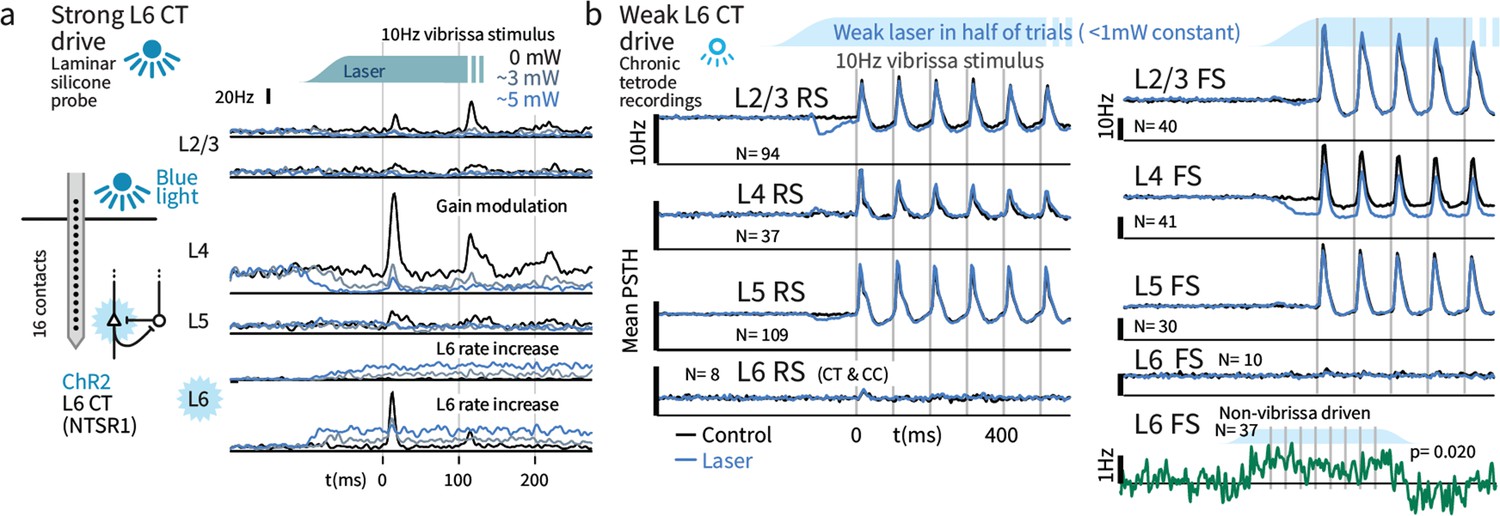
(a) Strong optogenetic L6 CT drive increased L6 firing rates and reduced sensory gain in other layers, as in visual neocortex (Olsen et al., 2012; Bortone et al., 2014), measured with laminar probes. Circuit diagram adapted from Olsen et al., 2012; Helmstaedter et al., 2008. (b) Chronic tetrode recordings across cortical layers. Low power (<1 mW) optogenetic drive did not change mean sensory evoked firing rate of RS in any layer, though a prestimulus change was observed in L2/3. Similarly, FS rates remained largely intact, with the exceptions that small firing rate changes were observed in L4 FS (decreased activity) and L6 FS that were not sensory responsive (increased activity).
-
Figure 4—source data 1
Extracellular electrophysiology responses.
- https://cdn.elifesciences.org/articles/48957/elife-48957-fig4-data1-v2.zip
-
Figure 4—source data 2
Extracellular electrophysiology spike data.
- https://cdn.elifesciences.org/articles/48957/elife-48957-fig4-data2-v2.zip
Figure 4—figure supplement 1
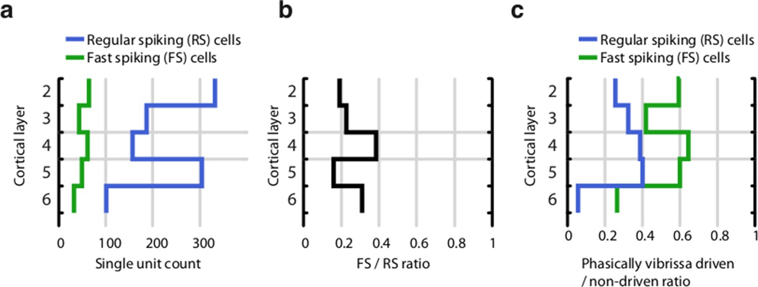
Proportion of fast spiking (FS) and regular spiking (RS) neurons across cortical layers.
(a) Total per-layer count of RS and FS cells. (b) Proportion of FS to RS cells across all layers. (c) Proportion of significantly vibrissa-stimulus driven (see Methods) RS and FS neurons across layers. The proportion of stimulus-driven cells is biased by our attempts to record from stimulus-driven cells – tetrodes were adjusted when recording conditions had stabilized but no stimulus-driven activity was recorded. Therefore, our data set likely significantly over-represents stimulus driven cells.
Figure 4—figure supplement 2
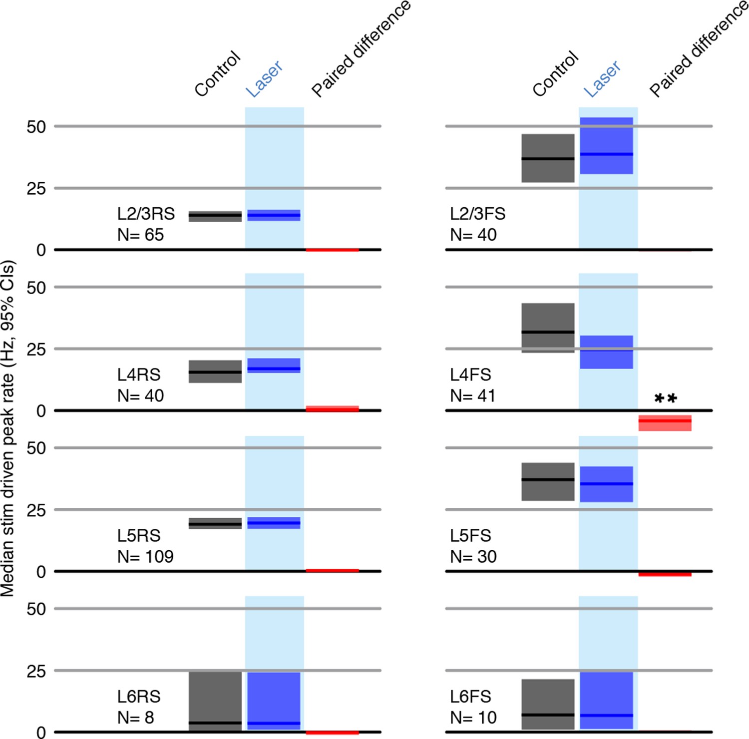
Peak firing rates (peak responses for deflections 2-7 for each neuron) for control and laser conditions across all stimuli.
All shaded error bars are 95% confidence intervals (CI) of the median.
Figure 5 with 2 supplements

Weak depolarization of L6 CT maintains overall rates but changes the identity of stimulus-driven ensembles in L6.
To test the impact of weak optogenetic drive on L6 CT, we combined optogenetic stimulation with awake 2-photon imaging using GCaMP6s expression in the L6-specific NTSR1-Cre line (see Materials and methods). (a) Example image of L6 CT somata, image summed over 12 individual frames, in each frame a subset of the cells were active. (b) An example Z-stack projection of GCaMP6s expression in L6 CT. (c) Sample frames from different depths of the Z-stack. (d) Example time series showing typical signal-to-noise ratios. (e) Optogenetic activation was interleaved with imaging at >200 Hz during laser scanning ‘flyback’. (f) Optogenetic drive did not significantly change the mean population response of L6 to sensory input, ranksum test, CI via bootstrap of median. (g) However, individual L6 cells showed significant facilitation or suppression of vibrissa-evoked responses during optogenetic drive. (h) Optogenetic L6 activation did not change the overall output from L6, but shifted the identity of the activated ensemble (p<0.001 IQR vs. shuffled control), regardless of whether cells were classified as vibrissa-driven in the control (red) or in the laser (blue) condition. Filled circles indicate cells where the laser effect was individually significant per-cell (p<0.0025, at 1 s time point, via bootstrap). Of cells that were sensory responsive in the laser condition, 25.0% were significantly facilitated, 23.9% suppressed, and of cells sensory responsive in the control condition, 10.9% were facilitated, 32.9% suppressed.
-
Figure 5—source data 1
L6 effect of weak optogenetic drive.
- https://cdn.elifesciences.org/articles/48957/elife-48957-fig5-data1-v2.zip
Figure 5—figure supplement 1
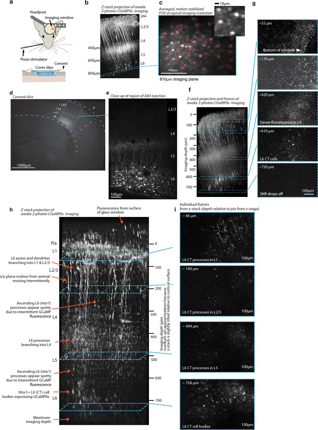
Histology and 2-photon imaging in L6 CT cells with GCaMP6s in the NTSR1-Cre line.
(a) Illustration of the imaging setup using two stacked cover slips under a bigger top cover slip. (b) Z-stack projection of GCaMP6s image stack acquired in awake animal. (c) Averaged, motion corrected field of view from typical L6 imaging session. (d) Coronal section (150μm thickness) imaged at 525nm showing AAV mediated expression of GCaMP6s in NTSR-1 positive L6 CT neurons. (e) Close-up of same slice (collage of 2 images), acquired with 2-photon scanning. (f) Z-stack assembled from 170 images at 5μm steps, shown slightly oblique (~10 degrees) to the imaging Z-axis, maximum intensity projection. The stack was acquired in a resting, awake animal. Overall features of the image are identical to panel a and b, but superficial fluorescence appears brighter due to the strong image intensity falloff at greater depths in the 2-photon z-stacks. Beady appearance of processes in superficial layers is due to intermittent calcium driven fluorescence that makes individual dendrites/axons show up as very bright, large spots in individual frames (see panel e, 2nd example frame). Note that the relatively weak and sparse fluorescence above L4 is much more visible here than in the slice. This lack of superficial fluorescence is likely one of the features of the NTSR1 line that make this deep 2-photon imaging possible (Ulanovsky et al., 2003). (g) Individual frames from Z-stack in panel f, each image is remapped to equalize contrast and brightness and slightly smoothed to improve visibility (gaussian filter, sigma=0.3px). (h) Z-stack, same procedure as in c, assembled from 165 images at 5μm steps. (i) Individual images from the z-stack in panel h.
Figure 5—figure supplement 2
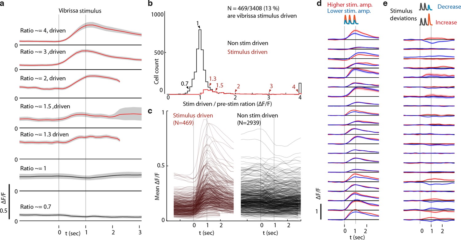
Classification of L6 CT cells as vibrissa-stimulus driven.
(a) Responses (stimulus triggered mean ΔF/F) for 7 example ROIs showing approximate stimulus drive ratios of 0.7, 1, 1.3, 1.5, 2,3, and 4. Stimulus drive amplitude was quantified as the ratio of the ΔF/F in a response window (0-2 seconds after vibrissal stimulus offset) divided by the baseline ΔF/F (-2 to 0 sec). Confidence bounds are 95% for mean via bootstrap. (b) Histogram of stimulus drive ratios for significantly vibrissa stimulus-driven (red) and non-driven (black) ROIs. ROIs were labeled as significantly stimulus driven if the 25th percentile of the mean ΔF/F in the response window was larger than the 95% percentile of the pre-stimulus period. (c) Mean responses for all stimulus-driven, and the first 500 non-significant ROIs. (d) Mean responses of highly stimulus-driven cells for high (red) and low (blue) (~120% or 80% of a mean stimulus amplitude) non-deviant vibrissa stimuli. (e) Mean difference between constant amplitude vibrissa stimuli and stimuli containing stimulus increase deviants (red) or decrease deviant.
-
Figure 5—figure supplement 2—source data 1
L6 calcium imaging sensory response statistics.
- https://cdn.elifesciences.org/articles/48957/elife-48957-fig5-figsupp2-data1-v2.zip
Figure 6

Small variations in baseline stimulus amplitude were not robustly encoded in layers 4 and 2/3 SI.
(a) Experimental preparation. Baseline stimulus amplitudes were varied by up to 15% on a trial-by-trial basis, in a range of ± ~ 25 mm/second, and presented in trains of 7 stimuli at 10 Hz. (b) The average sensory-evoked PSTHs from sensory-responsive RS neurons showed that neither L2/3 nor L4 cells significantly changed their mean firing rates to reflect stimulus amplitude in the range employed. (c) The population distribution of differences in spike rates per deflection between small and large baseline stimulus amplitudes showed no significant encoding of amplitude. Purple bars beneath each histogram indicate 95% CI (via bootstrap of median), ranksum test. (d) To probe the encoding of deviant presence, we presented amplitude deviations in the middle of stimulus trains. (e) To test for encoding of deviant presence, regardless of whether the deviants were increases or decreases in deflection amplitude, we calculated the average effect of deviants on firing (both types grouped, increases and decreases). While a few individual cells showed a generalized sensitivity to deviation, amplitude deviants did not systematically affect overall firing rates in L2/3 or L4, as shown in the centered population distribution.
-
Figure 6—source data 1
Spike data on effect of weak L6 drive on stimulus change representation.
- https://cdn.elifesciences.org/articles/48957/elife-48957-fig6-data1-v2.zip
Figure 7 with 1 supplement
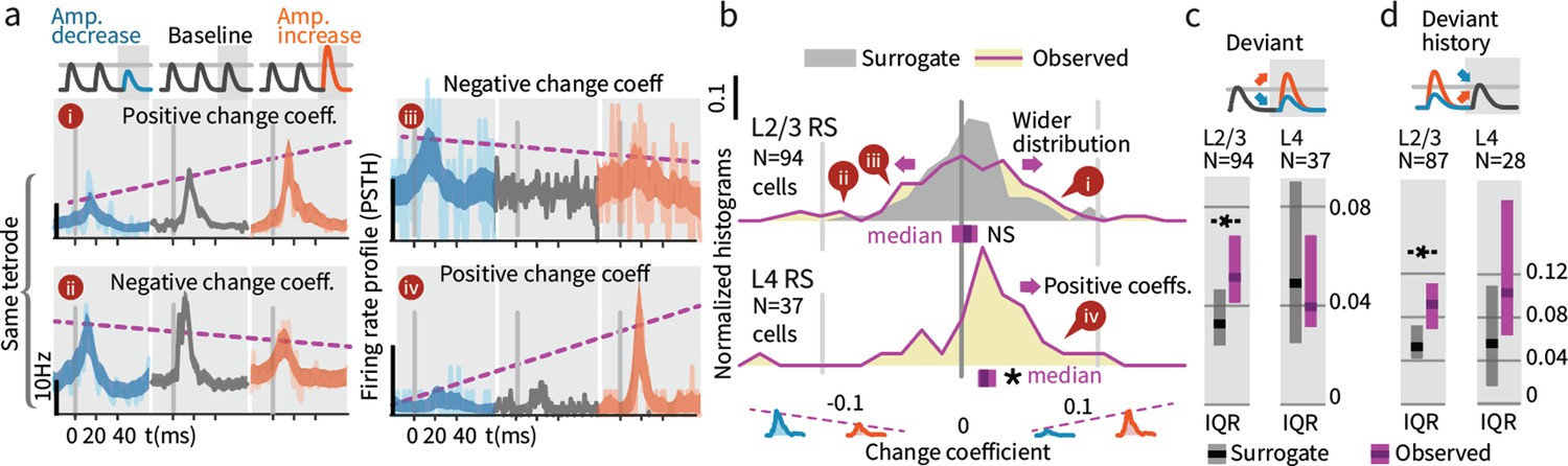
Small stimulus deviations were represented by distinct patterns of rate changes in layers 4 and 2/3.
(a) Stimulus amplitude deviants were presented after 2–6 repeated baseline amplitude stimulations. Examples show sensory-driven PSTHs, shaded regions indicate the 95% CI. Red traces are responses to amplitude increases, and blue to amplitude decreases, gray are baseline stimuli. We calculated a ‘change coefficient’, defined as spike count differences between responses to increased versus decreased amplitudes (purple dashed line). Neurons had diverse responses, including positive change coefficients (higher firing probability for stimulus increases - i, iv) and negative change coefficients (higher probability for stimulus decreases - ii, iii). (b) Histograms of the distribution of change coefficients for all stimulus-driven RS in L4 and L2/3. The L4 population responded to stimulus changes with positive change coefficients. In contrast, L2/3 showed several types of responses to deviants, with both positive and negative change coefficients, reflected in a broadening of the change coefficient distribution (purple) relative to a surrogate distribution of shuffled baseline stimuli (gray). Bars show the 95% CIs (purple) and the median value. (c) The L2/3 population, but not L4, was broader than a surrogate distribution, quantified via the interquartile range (IQR), ranksum test, bar graphs show median and 95% CI via bootstrap of median. (d) Heterogeneous encoding (reflected in broadening of the distribution) was also observed in L2/3 when initial baseline amplitudes were larger or smaller than a deviant that always had the same intermediate amplitude, demonstrating encoding of deviation from stimulus history and not absolute amplitude encoding in L2/3.
-
Figure 7—source data 1
Statistics on effect of weak L6 drive on stimulus change representation.
- https://cdn.elifesciences.org/articles/48957/elife-48957-fig7-data1-v2.zip
Figure 7—figure supplement 1

Method for matching positions in stimulus trains and for analysis of encoding of stimulus history.
(a) Possible positions of deviations in the stimulus train at deflections 2-7. (b) Distributions of positions in trains of baseline (grey) and deviant (red) stimuli. Baseline stimuli are more likely to occur at the beginning of the train (post-deviant stimuli were excluded from analysis). Overlapping region (dark brown) shows the subset of trials that was sampled from to compute surrogate distributions to compare baseline and deviant stimuli while controlling for possible effects of different N and different positions in train. (c) Stimulus design for sessions in which baseline amplitude was randomized across trials (N=55 sessions). (d) Selection of trials for analysis of neural encoding of stimulus changes. Green: analyzed stimuli. Baseline stimuli are compared to increased or decreased stimuli. For analyses that are affected by adaptation or different sample sizes, positional matching (see a, b) was used. (e) Selection of trials for analysis of stimulus history representation. Green: analyzed stimuli. Trials were sub-sampled to obtain conditions in which analyzed baseline amplitudes (grey) and deviant amplitudes (red/blue) were matched. The deviant condition was therefore defined by higher or lower preceding stimuli, allowing an analysis of the effects of stimulus history, independent of the current stimulus amplitude. For analyses that are affected by adaptation or different sample sizes, positional matching (see a, b) was used in addition to the amplitude matching.
Figure 8 with 2 supplements

Layer 6 pyramidal cells encoded stimulus amplitude.
(a) Activity in L6 neurons positively encoded stimulus amplitude, as reflected by larger signals among responsive neurons when the response to larger amplitude baseline stimuli was subtracted from the response to smaller baseline stimuli (N = 346 stimulus responsive neurons out of 2685 imaged). This finding contrasts with the encoding in L2/3 and 4, where we did not observe significant encoding of the baseline amplitude of the stimulus train (Figure 6). (b) L6 amplitude encoding was also observed when stimulus amplitude variation was provided by deviants later in the stimulus train. Blue/red indicate response to increases versus decreases in deviant amplitude relative to baseline. Because calcium imaging data were acquired at ~5 Hz, no attempt was made to quantify change onsets and only the post-stimulus window was analyzed. Bars show the 95% CIs (purple) and the median value. (c) Population data and summary statistics for L6 CT amplitude and change encoding.
Figure 8—figure supplement 1
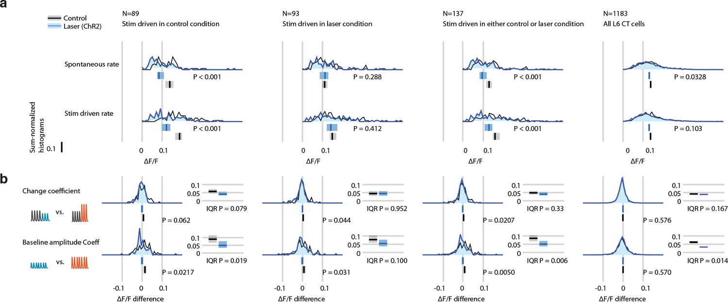
Weak optogenetic L6 CT drive with ChR2 disrupts encoding of small stimulus amplitude changes and deviants, quantified via raw ΔF/F.
Effect of weak L6 CT ChR2 drive (~0.1-0.2 mW through imaging window, see Figure 5) on L6 CT cell firing rates during vibrissa stimulation, measured by calcium imaging via GCaMP6s in stimulus driven cells. All vibrissa stimulus responses were quantified in a 0-2 sec window relative to stimulus offset (or equivalent time in catch trials). (a) Histogram of spontaneous (catch trials) or vibrissa stimulus evoked mean ΔF/F. Bar graphs show 95% CIs of the median per group via bootstrapping (1000 fold). P values are from two-sided Mann-Whitney rank sum tests between the control and laser conditions. Data is analyzed as all stimulus driven cells classified in control condition (left), classified in laser trials (middle left), in either condition (middle right), and for all L6 CT cells (far right). (b) Histograms of change coefficient, computed as the difference in evoked ΔF/F between constant and increasing amplitude and constant and decreasing amplitude trials, and baseline amplitude encoding (mean difference in ΔF/F between low and high-amplitude constant stimuli). Analysis is split into groups as in panel a. P values are either from Mann-Whitney rank sum tests (unpaired) or Wilcoxon sign rank test (paired by cell). Spread of the distributions is quantified via IQR, CIs are computed via 1000 fold bootstrap, P values via rank sum test.
-
Figure 8—figure supplement 1—source data 1
L6 stimulus and deviant encoding in control and weak L6 drive conditions.
- https://cdn.elifesciences.org/articles/48957/elife-48957-fig8-figsupp1-data1-v2.zip
Figure 8—figure supplement 2
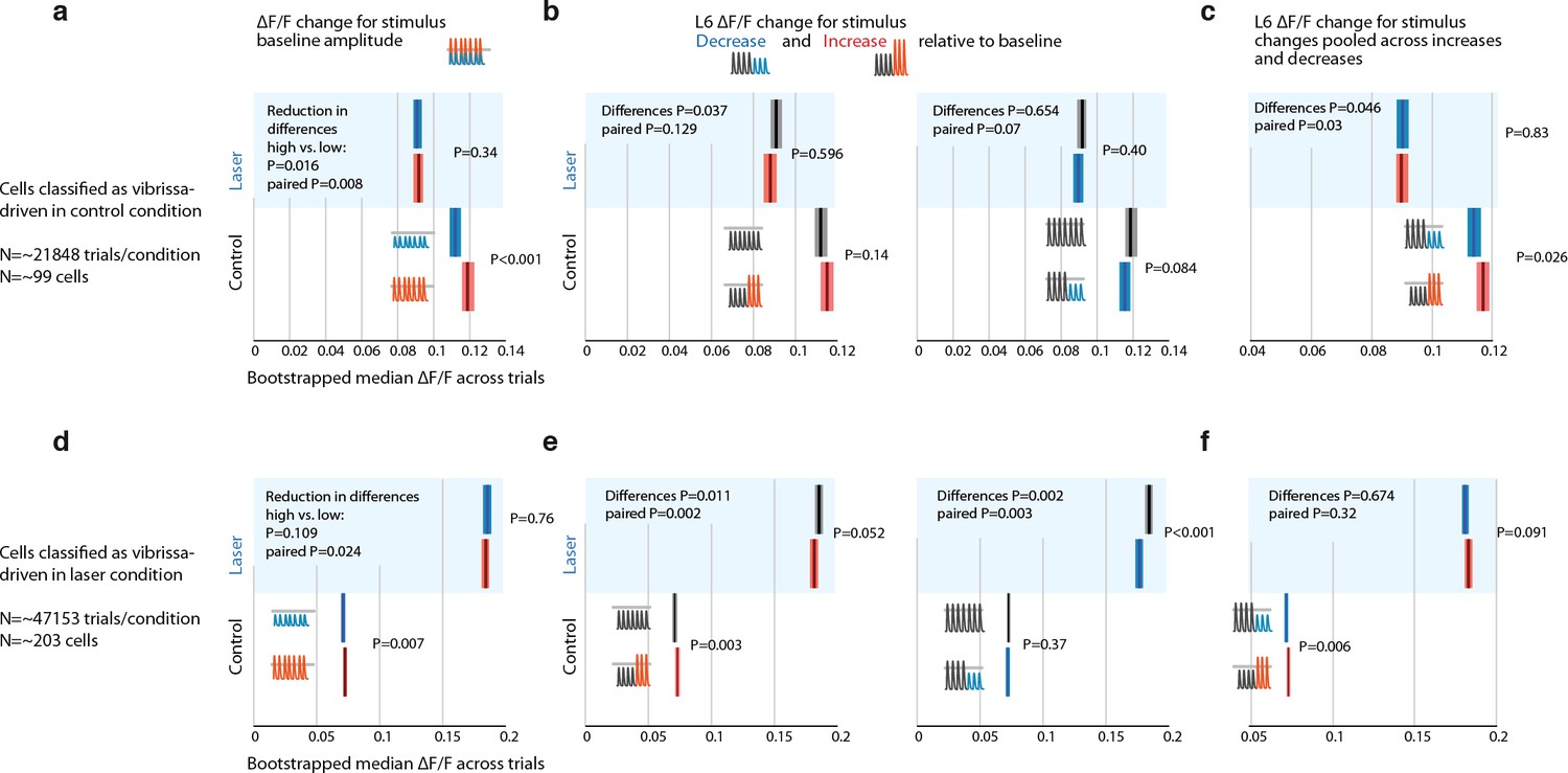
Weak optogenetic L6 CT drive with ChR2 disrupts encoding of small stimulus amplitude changes and deviants, quantified via leave-one-out cross-validation for stimulus driven vs. non-driven cells.
Effect of weak L6 CT ChR2 drive (~0.1-0.2 mW through imaging window, see Figure 5) on L6 CT cell firing rates during vibrissa stimulation, measured by calcium imaging via GCaMP6s in stimulus driven cells. All vibrissa stimulus responses were quantified in a 0-2 sec window relative to stimulus offset (or equivalent time in catch trials). (a) To test whether the encoding of stimulus features in L6 CT cells was affected by weak L6 drive independently of a possible selection bias in choosing cells that are stimulus driven in the control condition and then possibly lose significance in the laser condition purely because of the variance in their responses, we used a leave-one-out (LOO) method to quantify L6 CT cell responses (also used for quantifying the directional tuning on L6 CT cells). Instead of assigning cells as stimulus or not stimulus driven, we classified a cell as stimulus driven per trial, using all but one trial, and then analyzed this trial only if the other trials showed significant stimulus drive. This procedure avoids selecting data on the same dataset as is used for the analysis. In this analysis, positive change coefficients were observed (small stimuli led to smaller, bigger stimuli to bigger ΔF/F). P values for comparisons within control or laser conditions are from rank sum tests. This difference is significantly reduced in the laser condition. P values for the decrease of this difference, in control versus laser trials are computed by bootstrapping across trials and testing the median of the difference (laser vs. control) of differences (large in control-small in control) – (large in laser-small in laser) versus zero for each sample. For paired P values by cells, each bootstrap sample computed differences of the difference of mean responses as before, but within cells, for a bootstrapped sample of cells and then tested the median across cells versus zero. (b) Comparison of ΔF/F for constant and changing stimuli for increasing (red) and decreasing (blue) trials. (c) Same data as in panel d but pooled across increasing and decreasing deviant conditions. Deviants were significantly encoded and this encoding was disrupted in the laser condition. Because of the timescale of GCaMP6s, multiple interpretations exist for this encoding. This encoding may be determined by a delayed response to repeated presentation of the deviant amplitude and does not necessarily represent a true deviant encoding. (d,e,f) Same as panels c, d, e but cells were classified as stimulus driven (via LOO procedure) in the laser condition. Baseline stimuli are significantly encoded in these cells, and this encoding is significantly disrupted in the laser condition. Stimulus deviants are encoded in the control condition but the encoding is not reduced as clearly in the laser condition.
Figure 9 with 3 supplements
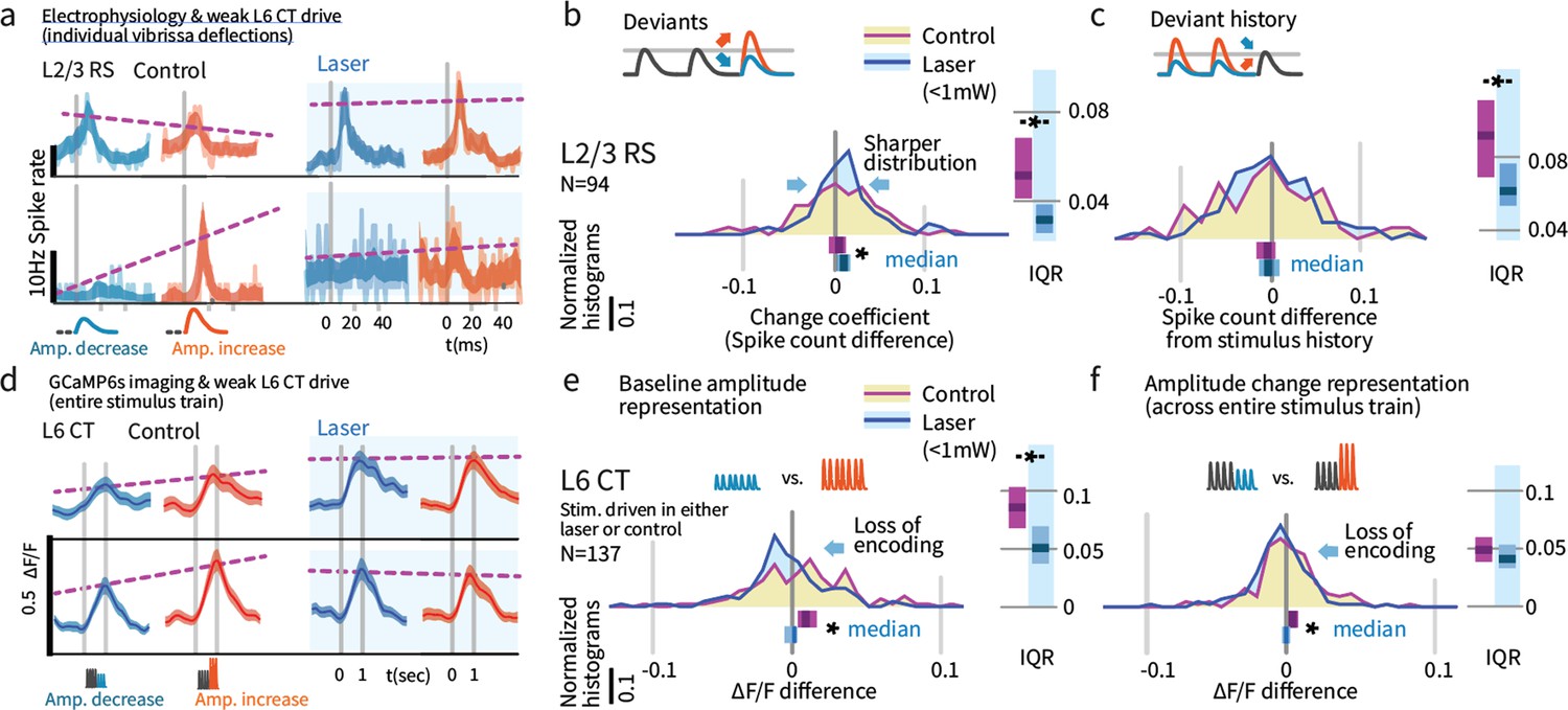
Weak L6 drive disrupts stimulus encoding in L6 and the emergence of deviant encoding in L2/3.
(a) Examples of L2/3 deviant encoding that were reduced with L6 optogenetic drive, of positive and negative sign. (b) Across the L2/3 population, weak L6 CT drive caused a loss in the heterogeneity of L2/3 encoding of deviants, reflected as a sharpening of the distribution and a bias to positive change coefficients, paralleling L4 encoding. Bar graphs show the 95% CI and the median value for the distribution, and for its interquartile range (IQR), via bootstrap. (c) Encoding of stimulus history in L2/3 was similarly disrupted. (d) Examples of L6 CT sensory responses (via Ca2+ imaging, see Figures 5 and 8) with and without optogenetic stimulation. In these examples, weak L6 CT optogenetic drive disrupted the representation of stimulus amplitude. (e) Population distributions show the loss of baseline amplitude encoding in L6 CT, and (f) loss of amplitude encoding for changes within the stimulus train.
Figure 9—figure supplement 1
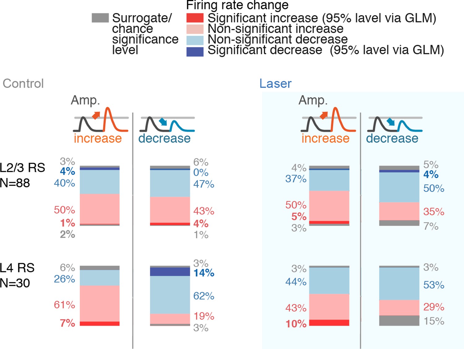
GLM coefficient statistics across layers and conditions.
Percentages of neurons with significantly increased or decreased firing rates, split by stimulus increases or decreases (each group rounded to nearest integer, as such totals do not necessarily add to 100%). Same analysis was run for control and laser conditions. The shift away from heterogeneous deviant encoding in L2/3 RS in the laser conditions is reflected in the higher proportion of positive coefficients. Significance of individual neurons was assessed using a GLM, using a 95% significance level at ~500 trials. The (relatively small) numbers of individually significant neurons using this criterion do therefore not reflect the information content of their spike output, but should be interpreted only in their difference across layers, cell types and control versus laser conditions. In L2/3, population-level analysis of deviant encoding shows robust encoding of deviants via the variance of their change coefficients and via ideal observer analysis (Figure 9, Figure 9—figure supplement 2).
Figure 9—figure supplement 2
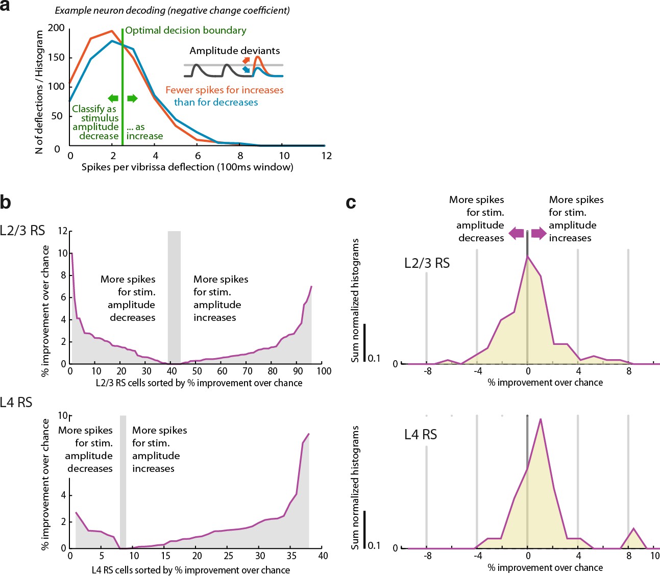
L2/3 RS cells encode stimulus amplitude deviant identity heterogeneously, in contrast to L4.
L2/3 has an equal proportion of cells with increased or decrease firing probability for stimulus amplitude increases, in contrast to L4. This mirrors the same finding obtained by directly analyzing firing probability for increase/decrease deviants (Figure 7). (a) Example of ideal observer decoding for one cell. A optimal spike threshold is chosen as the value that results in the best classification rate (maximally different from 50%). Higher spike counts were always decoded as stimulus increases. For cells that decrease their firing rate for increased stimulus amplitudes or vice versa (i.e., negative change coefficient neurons), the correct rate would therefore be <50%. A cell that fires on every trial with a significantly positive change coefficient could theoretically result in a 100% classification rate, while such a cell with negative change coefficient could yield an (equally informative) 0% hit rate. (b) Rectified (always positive) correct classification rates relative to chance rate (which can slightly differ from 50% because of unequal proportions of stimulus increase versus decrease trials). In L4, most cells showed positive classification rates / spike count increases for stimulus increases, while in L2/3 the proportions are closer to even.c,Histogram of (non rectified) correct rates relative to chance level across cells – the distribution of cells with positive or negative change encoding mirrors that of the change coefficients (Figure 7).
Figure 9—figure supplement 3
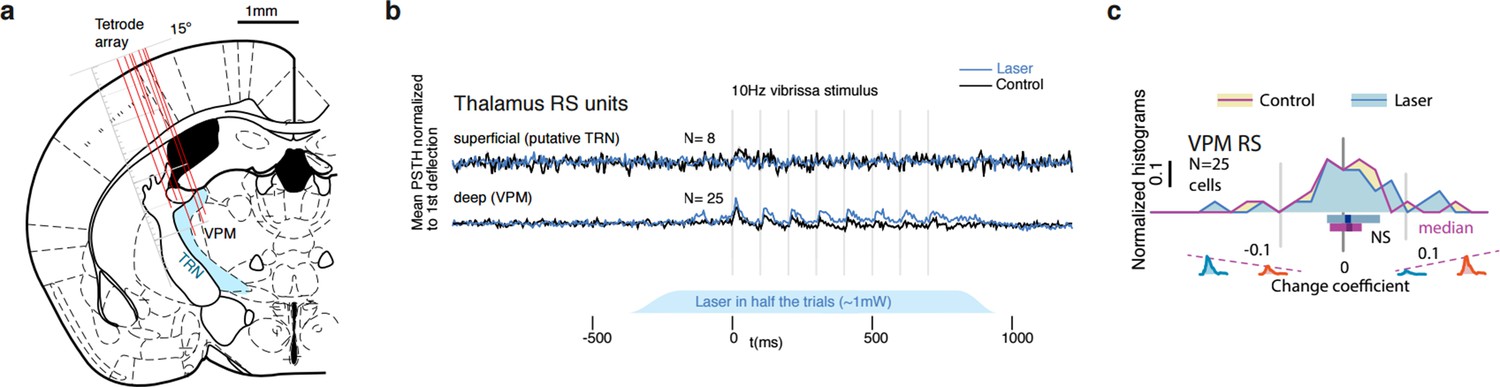
Thalamic relay cells do not encode stimulus deviants as significantly as cortical L4 RS cells.
(a) We recorded a total of 240 putative VPM cells. Recording locations in VPM and neighboring TRN are shown for one animal. (b) Out of the sample of VPM cells, 25 cells were significantly phasically stimulus driven. We also observed 8 TRN neurons with weak stimulus -onset specific firing. (c) Same analysis as Figure 7 – Neither in the control condition or under weak L6 drive are stimulus deviants encoded in the recorded VPM cells. TRN cells were not phasically stimulus driven past the first deflection and carried no stimulus information.
Figure 10
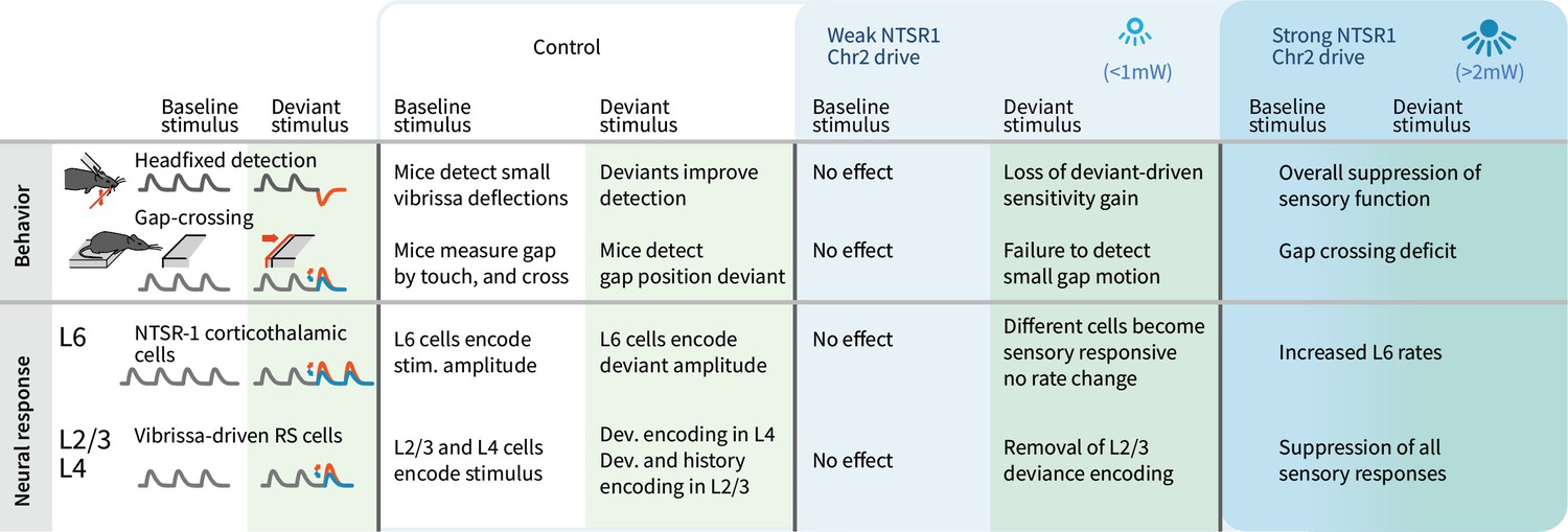
Summary of main findings.
The effects of strong vs. weak drive of L6 CT neurons on behavior and on the electrophysiological signatures of baseline and deviant stimuli.
Videos
Video 1
Mouse crossing in the Gap Crossing with deviation task.
Example raw videos from two trials. Left: Weak L6 drive leads to mice not reacting to sudden small platform position deviations. Right: Control trial, mice slow down their approach in reaction to sudden platform position deviations. Inserts show target distance over time.
Additional files
Download links
A two-part list of links to download the article, or parts of the article, in various formats.
Downloads (link to download the article as PDF)
Open citations (links to open the citations from this article in various online reference manager services)
Cite this article (links to download the citations from this article in formats compatible with various reference manager tools)
Layer 6 ensembles can selectively regulate the behavioral impact and layer-specific representation of sensory deviants
eLife 9:e48957.
https://doi.org/10.7554/eLife.48957


