Figures and data in From plasmodesma geometry to effective symplasmic permeability through biophysical modelling

Version of Record

Accepted for publication after peer review and revision.

Download
Cite
Share
CommentOpen annotations (there are currently 0 annotations on this page).

Version of Record published: January 31, 2020 (This version)
Accepted Manuscript updated: November 25, 2019 (Go to version)
Accepted Manuscript published: November 22, 2019 (Go to version)
Accepted: November 16, 2019
Received: June 3, 2019

Figures
Tables
Additional files

12 figures, 3 tables and 2 additional files

Figures

Figure 1

Download asset Open asset

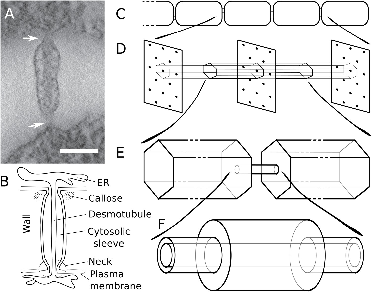
Modelling effective symplasmic permeability: concept overview.

(A) Electron microscopy image showing one PD, constricted at the neck regions (arrows), from *Arabidopsis thaliana* root tissue. The image was extracted from a reconstructed tomograph. Scale bar: 50 nm. The image was kindly provided by the Bayer lab. (B) Cartoon showing PD geometry and structural features. (**C-F**) The model to determine effective symplasmic permeability considers that connectivity within a cell file (C) is affected by the distribution of PDs in the cell wall (D) (modelled as a function of the cytoplasmic column belonging to a single PD (E)) as well as by the structural features of individual PDs (F).

Figure 2

Download asset Open asset

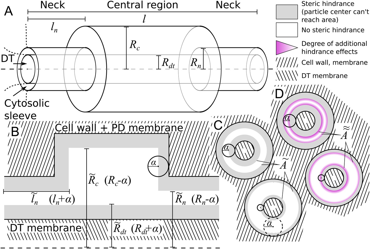
Model PD geometry and hindrance effects.

(A) Individual PDs are modelled using multiple cylinders with a total length $l$ , neck (inner) radius $R_{n}$ and neck length $l_{n}$ , central region (inner) radius $R_{c}$ and desmotubule (outer) radius $R_{d t}$ . B,C: Illustration of the impact of steric hindrance and rescaled parameters. The gray areas of the longitudinal (B) and transverse (C) sections cannot be reached by the center of the particle with radius $α$ (steric hindrance). For a concise description of the available volume and cross section area, we use the rescaled lengths ${\tilde{l}}_{n} = l_{n} + α$ , ${\tilde{R}}_{c} = R_{c} - α$ , ${\tilde{R}}_{d t} = R_{d t} + α$ and ${\tilde{R}}_{n} = R_{n} - α$ . (C) The cross section area available for diffusion on a transverse section was named $\tilde{A}$ , which depends on the particle radius ( $α$ ). $\tilde{A}$ is the area of the white ring in each cross section. The maximum particle size $\bar{α}$ is illustrated with a dashed circle. For a particle of size $α = \bar{α}$ , $\tilde{A} = 0$ . (D) In practice, particles spend less time diffusing close to the wall than farther away from it (hydrodynamic hindrance). Consequently, the area close to wall contributes less to diffusive transport, as illustrated with purple gradients. These additional hindrance effects are accounted for in $\tilde{\tilde{A}}$ .

Figure 3 with 1 supplement

Download asset Open asset

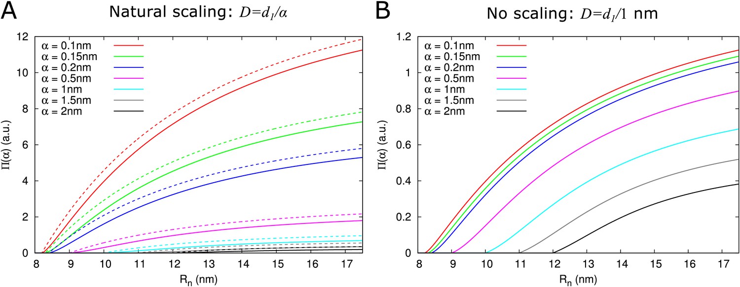
Impact of particle size (radius = $α$ ) on single pore effective permeability $Π (α)$ .

(A) Dependence of $Π (α)$ on neck radius ( $R_{n}$ ) and $α$ (different line colours, see legend). The diffusion constant $D$ is inversely proportional to particle size ( $D = d_{1} / α$ ). Dashed lines show $Π (α)$ considering only steric hindrance, solid lines include all hindrance effects. B: Using the same diffusion constant for all particle sizes instead shows that, once particles can pass easily, the particle size dependence of $Π (α)$ is largely due to the relation between particle size and diffusion constant. Parameters for calculations: $l$ = 200 nm, $l_{n}$ = 25nm, $R_{d t}$ = 8 nm, $R_{c}$ = 17.5 nm. For simplicity we use $d_{1}$ = 1 nm³/s in this figure. Therefore, only the relative values of the unit permeabilities have meaning (consequently expressed in arbitrary units [a.u.]).

Figure 3—figure supplement 1

Download asset Open asset

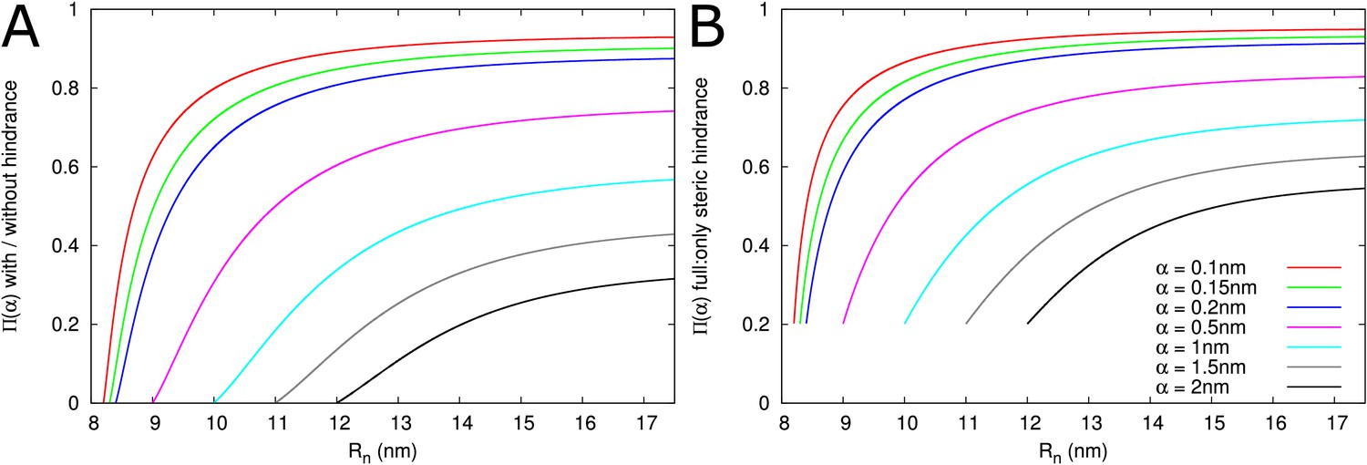
Impact of hindrance effects on $Π (α)$ .

(A) Impact of hindrance on $Π (α)$ decays with decreasing relative particle size. (B) Steric hindrance alone particularly overestimates $Π (α)$ for large relative particle sizes. Parameters: $l$ = 200 nm, $l_{n}$ = 25nm, $R_{d t}$ = 8 nm, $R_{c}$ = 17.5 nm.

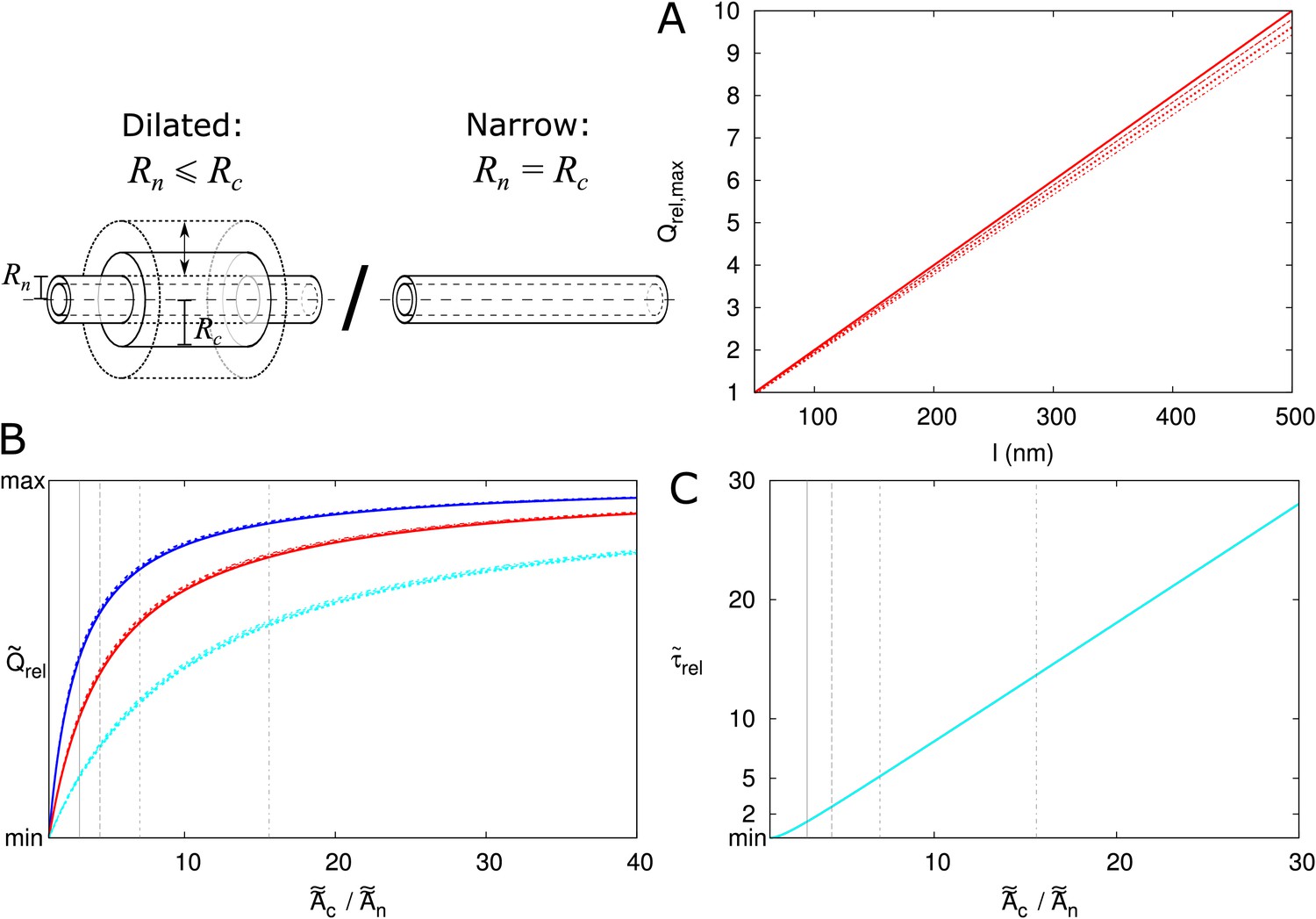
Figure 4 with 2 supplements

Download asset Open asset

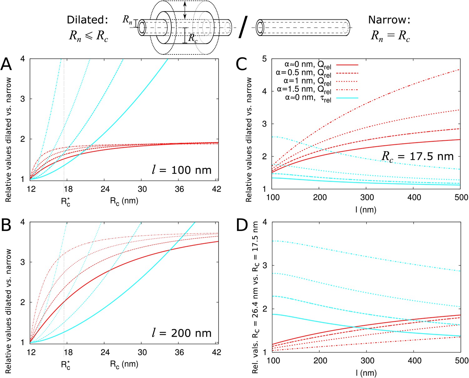
Impact of central region dilation on molar flow rate ( $Q$ ) and mean residence time ( $τ$ ).

The same legend shown in C applies to all panels. Narrow channels have $R_{n} = R_{c} =$ 12 nm, whereas for necked/dilated channels, $R_{n}$ = 12 nm but $R_{c}$ varies. (**A-C**) Red curves show the relation between molar flow rate in dilated PD vs narrow PD $Q_{r e l} = Q_{d i l a t e d} (R_{n}, R_{c}) / Q_{n a r r o w} (R_{n})$ whereas cyan curves show the relation between mean residence time in dilated PD vs narrow PD: $τ_{r e l} = τ_{d i l a t e d} (R_{n}, R_{c}) / τ_{n a r r o w} (R_{n})$ . Both quantities are computed for different particle sizes (solid: $α \approx 0$ , dashed: $α$ = 0.5 nm, sparse dashed: $α$ = 1 nm, dash-dotted: $α$ = 1.5 nm). (**A, B**) $Q_{r e l}$ and $τ_{r e l}$ are shown as a function of the radius in the central region $R_{c}$ for different PD lengths (cell wall thickness) (A) $l$ = 100 nm, (B) $l$ = 200 nm. (C) Values calculated for $R_{c}$ = 17.5 nm ( $R_{c}^{*}$ in A,B) as a function of PD length. (D) Ratios of curves calculated for $R_{c}$ = 17.5 nm (C) and $R_{c}$ = 26.4 nm (Figure 4—figure supplement 1B) represented for varying PD lengths. Other parameters used for modelling are: $l_{n}$ = 25 nm, $R_{n}$ = 12 nm, $R_{d t}$ = 8 nm.

Figure 4—figure supplement 1

Download asset Open asset

Additional panels: $l$ = 500 nm (similar to **A, B**), $R_{c}$ = 26.4 nm (similar to C).

Additional panels for Figure 4: Impact of central region dilation on molar flow rate ( $Q$ ) and mean residence time ( $τ$ ). (A) $R_{c}$ variable, $l$ = 500 nm, compare to Figure 4A,B. (B) $R_{c}$ = 26.4 nm, $l$ variable, compare to Figure 4C.

Figure 4—figure supplement 2

Download asset Open asset

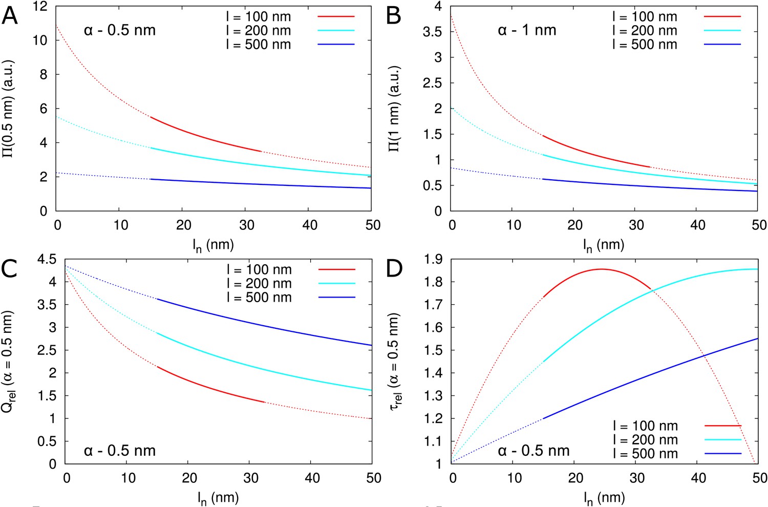
Impact of neck length $l_{n}$ on $Π (α)$ , $Q_{r e l}$ and $τ_{r e l}$ .

(**A, B**) Dependence of $Π (α)$ on $l_{n}$ for different PD length (indicated by line colour) for $α$ = 0.5 nm (A) and $α$ = 1 nm (B). Dotted lines indicate that neck length is unrealistically short ( $l_{n} <$ 15 nm), or the central region is too short for computations to be considered valid (conservatively estimated as $l - 2 l_{n} < 2 R_{c}$ ). (C) Dependence of $Q_{r e l}$ on $l_{n}$ for different PD length (line colours as in A). (D) Dependence of $τ_{r e l}$ on $l_{n}$ for different PD length (line colours as in A). (**C, D**) Except for the scaling of the y-axis, curves for different particle sizes are highly similar. Default parameters: $R_{n}$ = 12 nm, $R_{c}$ = 17.5 nm, $R_{d t}$ = 8 nm.

Figure 5 with 1 supplement

Download asset Open asset

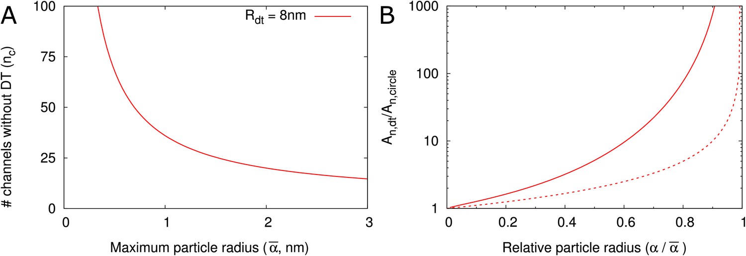
DT increases the cross section surface area available for transport per channel given a maximum particle radius $\bar{α}$ .

(A) The number of cylindrical channels ( $n_{c}$ ) that is required to match the total entrance surface of a single channel with $R_{d t}$ = 8 nm and the same maximum particle radius $\bar{α}$ . (B) Shows the relative area available for transport ( $A_{n}$ ) in relation to relative particle size ( $α / \bar{α}$ ) when comparing channels with DT and the equivalent number of cylindrical channels. Total surface area is the same. Solid lines include all hindrance effects ( ${\tilde{\tilde{A}}}_{n} {}_{, d t}/ {\tilde{\tilde{A}}}_{n}_{, c i r c l e}$ ; cf. Figure 2D). Dashed lines includes steric effects only ( ${\tilde{A}}_{n, d t} / {\tilde{A}}_{n, c i r c l e}$ ; cf. Figure 2C).

Figure 5—figure supplement 1

Download asset Open asset

Hindrance factors with and without DT.

Hindrance factors for slit (‘with DT’) and cylinder (‘no DT’) compared.

Figure 6 with 1 supplement

Download asset Open asset

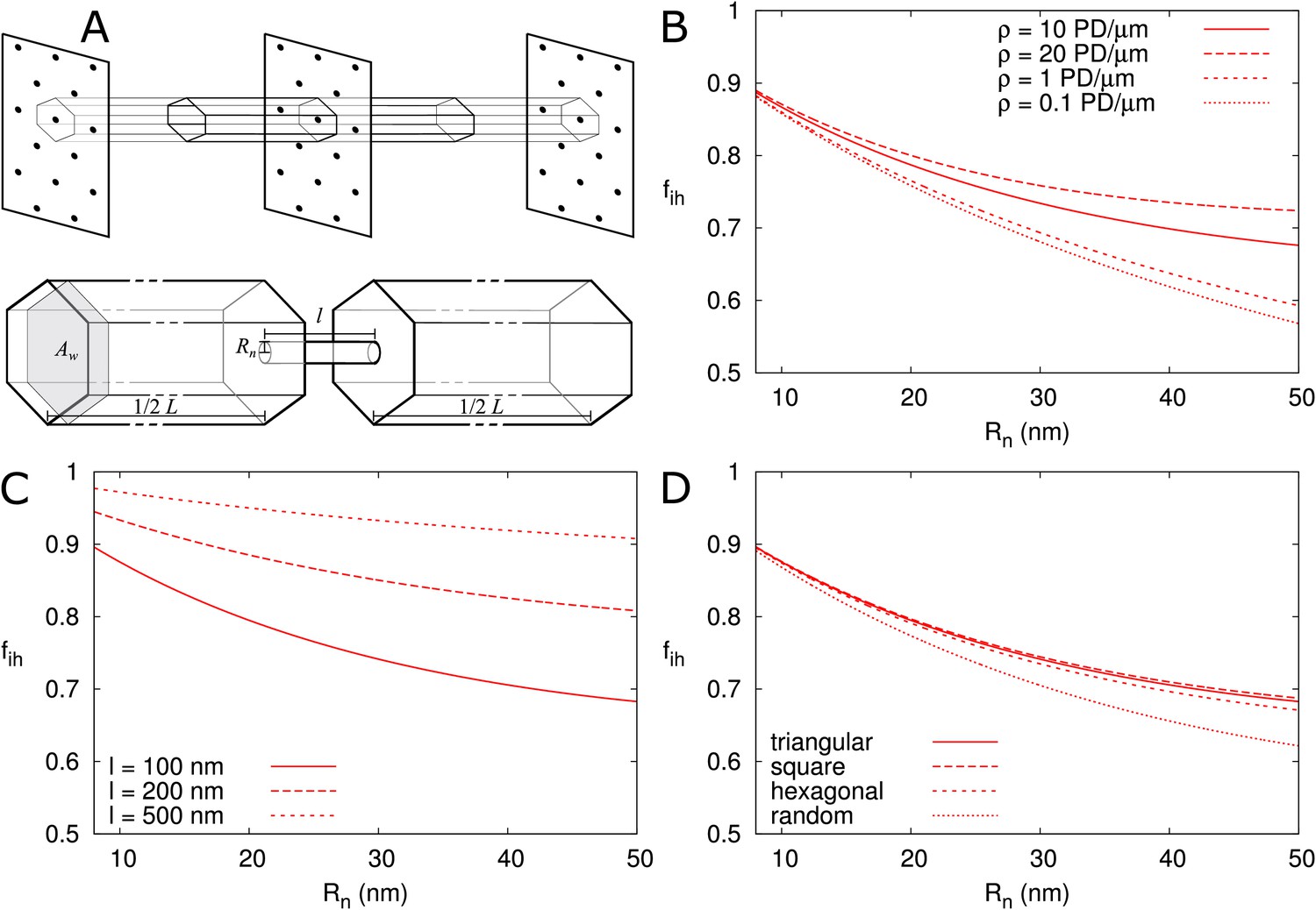
Correction factor $f_{i h}$ for inhomogeneous wall permeability depends on PD distribution, cell wall thickness and neck radius.

(A) The cartoon shows the geometrical considerations and parameters used to model the diffusion towards PDs. Cell wall inhomogeneity is incorporated as a correction factor $f_{i h}$ , $0 < f_{i h} \leq 1$ , which measures the relative impact of cytoplasmic diffusion towards the locations of the PDs in the cell wall compared to reaching a wall that is weakly but homogeneously permeable (i.e., with $f_{i h} = 1$ ). The cytoplasm is considered homogeneous. Each bit of cytoplasm can be assigned to the PD closest to it. With PDs on a regular triangular grid, the cytoplasm belonging to a single PD, with an outer (neck) radius $R_{n}$ , is a hexagonal column with cross section area $A w$ and 1/2 of the cell length $L$ on either side of the wall. (**B-D**) $f_{i h}$ is represented as a function of $R_{n}$ . The presence/absence of DT does not affect the values of $f_{i h}$ (Figure 6—figure supplement 1A). In all cases, solid lines correspond to: $l$ = 100 nm, $L$ = 10 μm, $α$ = 0.5 nm, a PD density of $ρ$ = 10 PD/μm², and PDs distributed on a triangular grid. Broken lines show the effects of changes in PD density $ρ$ (B), PD length $l$ (C) and PD distribution (D).

Figure 6—figure supplement 1

Download asset Open asset

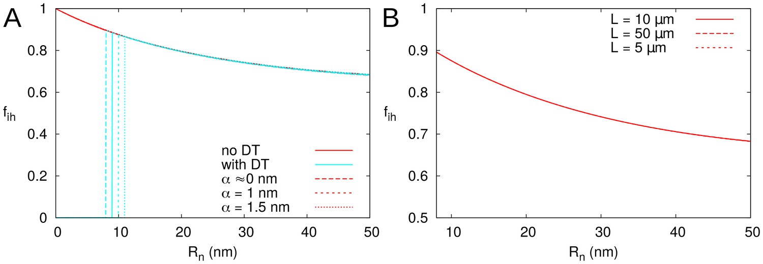
$f_{i h}$ is not affected by particle size $α$ , presence of DT, or cell length $L$ .

$f_{i h}$ is represented as a function of $R_{n}$ , calculated for PDs with (cyan; A only) and without (red) DT. In all cases, solid lines correspond to: $l$ = 100 nm, $L$ = 10 μm, $α$ = 0.5 nm, a PD density of $ρ$ = 10 PD/μm², and PDs distributed on a triangular grid. Broken lines show the effects of changes in particle size $α$ (A) or cell length $L$ (B). Vertical cyan lines in A indicate the $R_{n}$ in which $f_{i h}$ is start to be measurable as determined by $α < \bar{α}$ .

Figure 7

Download asset Open asset

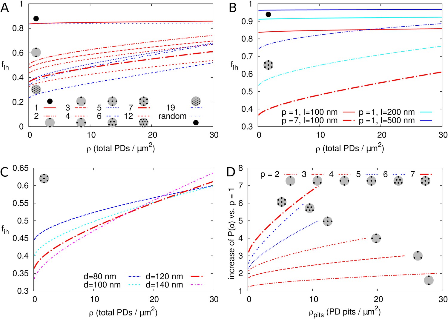
Impact of PD clustering into pit fields.

PD organization within pits is indicated with small cartoons in each graph. Pits themselves are distributed on a regular triangular grid. Within pit fields, the nearest neighbour distance between PDs $d$ (120 nm by default) is independent of the number of PDs per pit field. (**A-C**) $f_{i h}$ is represented as a function of total PD density $ρ$ (the total number of PD entrances per unit of cell wall area) for: a varying number of PDs per cluster $p$ (as indicated by line type, (A), for different PD length $l$ (B, solid lines: isolated PDs, dash-dotted lines: 7 PDs per cluster, red colour indicates $l$ : 100 nm, cyan for 200 nm, blue for 500 nm) and for different PD spacing within clusters (C, shown for clusters of 7 PDs with centre-to-centre distance $d$ as indicated by line type and colour). Cluster sizes 5, 6, and 19 are indicated with blue lines for readability (**A,D**). For comparison, $f_{i h}$ for non-clustered but randomly distributed PDs is also indicated. (D) The impact of increasing the number of PDs per cluster $p$ on $P (α)$ as a function of cluster density $ρ_{p i t s}$ (the number of pit fields per unit of cell wall area). Lines show the fold increase of $P (α)$ when increasing the number of PDs per cluster from one to the number indicated by the line type (same as in A). Lines are terminated where $f_{i h}$ of clusters meets $f_{i h}$ of isolated PDs at the same total PD density. Beyond that, calculation results are no longer reliable because clusters get too close and the impact of clustering on $f_{i h}$ could be considered negligible. (**A-D**) Default parameters: $l$ = 100 nm, $d$ = 120 nm, $R_{n}$ = 12 nm.

Figure 8

Download asset Open asset

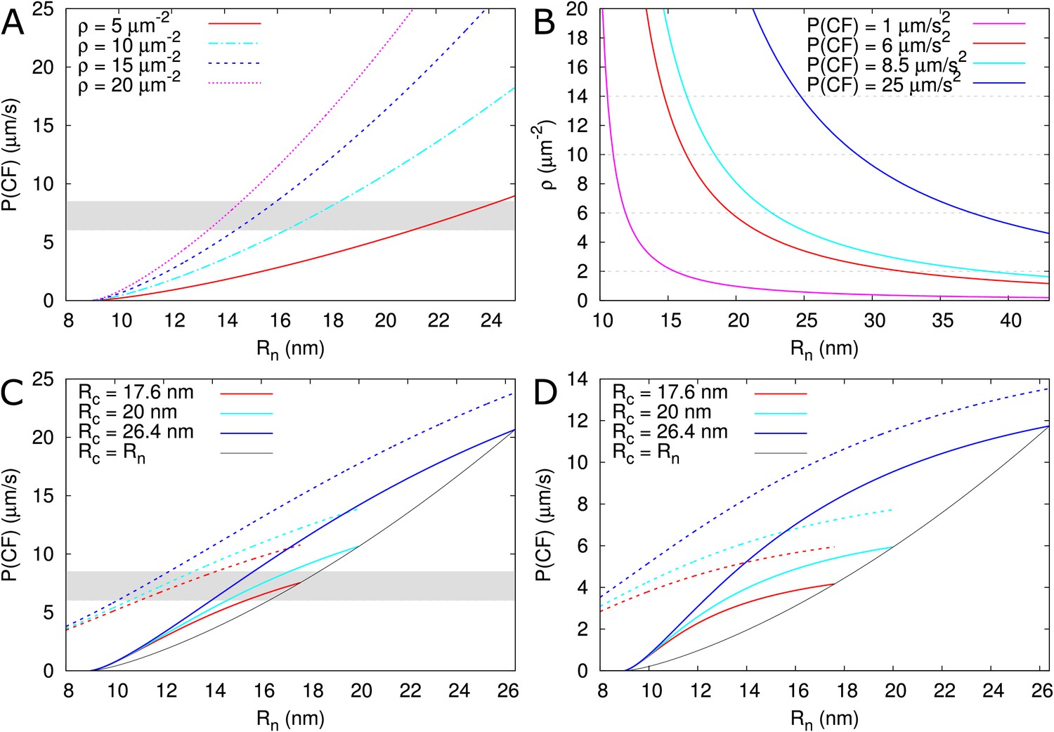
Calculated effective permeabilities for carboxyfluorescein (CF) as a function of PD aperture at the neck $R_{n}$ .

(**A, B**) Shows the graphs for straight channels. (A) Effective permeabilities are calculated for different PD densities (different colour curves). The horizontal gray band in A and C indicates the cortical values observed by Rutschow et al. (2011). (B) Shows the PD density required to obtain measured values of $P (C F)$ (different colour curves) as a function of $R_{n}$ . Horizontal broken lines are introduced to aid readability. (**C, D**) Shows that effective permeability increases with dilation of the central region ( $R_{c} > R_{n}$ ). As a reference, values for straight channels are indicated in black. Dashed curves show values calculated for channels without DT. (D) Shows the same calculations as C but for longer PDs $l$ = 200 nm. Default parameters: $α$ = 0.5 nm, $D$ = 162 μm²/s, $l_{n}$ = 25 nm, $l$ = 100 nm, $R_{d t}$ = 8 nm, $ρ$ = 10 PD/μm², PDs are spaced on a triangular grid, without clustering.

Appendix 2—figure 1

Download asset Open asset

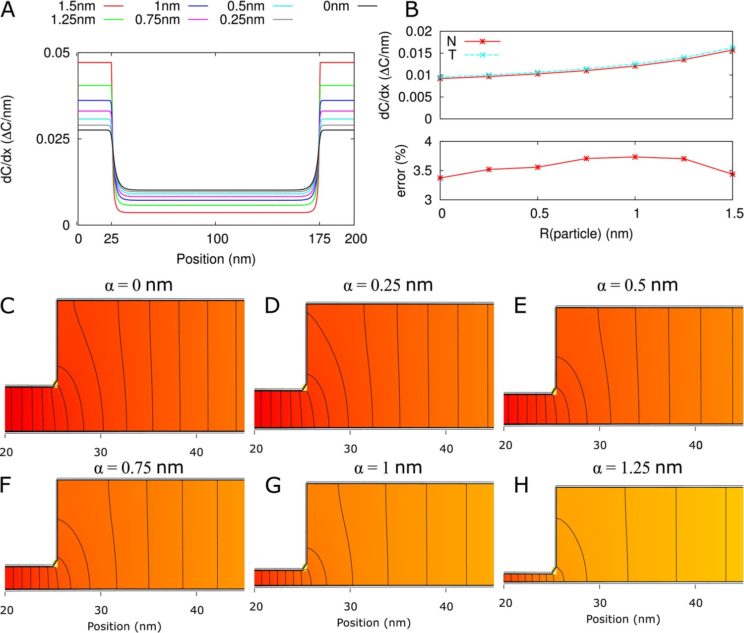
Error of homogeneous flux approximation (all 2D).

(A) $\partial C / \partial x$ from numerical calculations (2D) along a straight line through the middle of the available neck region for different particle sizes. (B) Top: $\partial C / \partial x$ at neck entrance (proportional to the channel flux) from numerical calculations (N; solid red line with asterisks) and from 3-cylinder model with homogeneous flux assumption (T; dashed cyan line with crosses). The 3-cylinder model results in a consistent over estimation of < 4% (bottom). (**C-H**) Concentration heat maps for available part of the channel, focus on the neck/central region transition. The same color gradient is used for all six graphs. Black isolines are spaced at 1% of the total concentration difference over the channel. Parameters: $l$ = 200 nm, defaults.

Appendix 2—figure 2

Download asset Open asset

Comparison of $τ_{r e l}$ as used in the main text against a $τ_{∥, P D}$ based calculation ( $τ_{∥, r e l}$ ).

$l$ = 100 nm, $R_{n}$ = 12nm, $R_{d t}$ = 8 nm, $l_{n}$ = 25 nm.

Appendix 3—figure 1

Download asset Open asset

Scaling of $Q_{r e l}$ and $τ_{r e l}$ through the PD.

(A) Maximum possible increase of $Q$ . Line type indicates particle size (solid: $α \approx 0$ , dashed: $α$ = 0.5 nm, sparse dashed: $α$ = 1 nm, dash-dotted: $α$ = 1.5 nm). (B) Curves for different $α$ almost collapse with when plotted as function of ${\tilde{A}}_{c} / {\tilde{A}}_{n}$ and rescaled from the minimal value of 1 to $Q_{r e l, m a x}$ . The curves for different $l$ do not collapse (blue: $l$ = 100 nm, red: $l$ = 200 nm, cyan: $l$ = 500 nm). (C) Curves for $τ_{r e l}$ collapse (for different $l$ and $α$ ) with rescaling function ${\tilde{τ}}_{r e} = (τ_{r e l} - 1) l^{2} / (2 {\tilde{l}}_{n} (l - 2 {\tilde{l}}_{n}))$ . Vertical lines in B,C correspond to ${\tilde{\tilde{A}}}_{c} / {\tilde{\tilde{A}}}_{n}$ for different particle sizes (line types as in A). Parameters: $l_{n}$ = 25 nm, $R_{n}$ = 12 nm, $R_{d t}$ = 8 nm.

Appendix 4—figure 1

Download asset Open asset

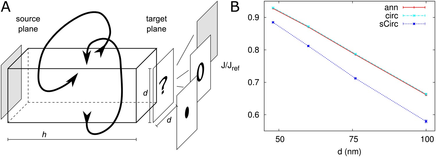
Correction factor for annular trap shape.

Comparison of discrete and homogeneous permeability. (A) Setup. A homogeneous source is located at a distance $h$ from a trapping plane with either a single trap or homogeneous absorbency. The periodic boundary conditions in the other directions make that the traps are effectively spaced on a square grid with distance $d$ between traps. (B) Relative average net flux in direction of trap (component along the box) for PDs with DT (‘ann’: red) and circular channels with the same apparent surface (‘sCirc’: blue) and same outer radius, but trapping rate decreased according to surface ratios (‘circ’: cyan), $h$ = 300 nm. For both, the flux is compared with a homogeneous trap with rate $κ = \frac{A_{a n n}}{A_{t o t a l}} D / μ m$ . Error bars (nearly invisible) represent the quality of the numerical estimate by minimum and maximum possible values.

Tables

Table 1

Pit radius ( $R_{p i t}$ ) as a function of number of PDs per pit.

The third and fourth column show numerical values for $d$ = 120 nm and $R_{n}$ = 12.

PDs/pit	$R_{p i t}$	$A_{P D} / A_{p i t}$	$R_{p i t}$
1	$R_{n}$	1	12
2	$R_{n} + \frac{1}{2} d$	0.056	72
3	$R_{n} + \frac{1}{3} \sqrt{3} d$	0.065	81.3
4*	$R_{n} + \frac{1}{2} \sqrt{2} d$	0.061	96.9
5*	$R_{n} + d$	0.041	132
6	$R_{n} + \frac{2}{3} \sqrt{3} d$	0.038	150.6
7	$R_{n} + d$	0.058	132
12	$R_{n} + \frac{1}{3} \sqrt{13} d$	0.071	156.2
19	$R_{n} + 2 d$	0.043	252

*: All entries are based on PDs on a triangular grid within each pit, except for 4 and 5, where the PDs inside a pit are arranged on a square grid. Clusters (pitfields) are always arranged on a triangular grid.

Table 2

Parameter requirements for reproducing measured $P (C F)$ values (Rutschow et al., 2011) with the default model.

This table was generated using PDinsight. A: Required density ( $ρ$ ) for a given $\bar{α}$ and neck radius ( $R_{n}$ ). B: Required $\bar{α}$ and corresponding $R_{n}$ for a given $ρ$ . C: values required to reproduce $P (C F)$ = 25 μm/s. Values computed for a 2x, 3x and 4x increase of $ρ$ are also shown. This is done both for a uniform increase of the density ( $p = 1$ ) and for (repeated) twinning ( $p > 1$ ) from a uniform starting density (indicated in bold). $p$ is the number of PDs per pit.

A $P (C F)$ (μm/s)	$\bar{α}$ (nm)		$R_{n}$ (nm)	$ρ$ (PD/μm²)
3.3*	2.0		12	18.6
	2.5		13	12.6
	3.0		14	9.3
	3.4		14.8	7.6
	3.5		15	7.3
	4.0		16	5.9
6	2.0		12	33.5
	2.5		13	22.7
	3.0		14	16.8
	3.4		14.8	13.8
	3.5		15	13.2
	4.0		16	10.7
8.5	2.0		12	47.2
	2.5		13	32.0
	3.0		14	23.7
	3.4		14.8	19.4
	3.5		15	18.5
	4.0		16	15.0
B $P (C F)$ (μm/s)	$ρ$		$\bar{α}$	$R_{n}$ (nm)
3.3*	5		4.5	16.9
			4.2	16.5
6	10		4.2	16.3
	13		3.5	15.1
8.5	10		5.2	18.4
	13		4.4	16.8
1	10		1.5	11.0
	13		1.3	10.6
C $P (C F)$ (μm/s)	$ρ$	$p$	$\bar{α}$	$R_{n}$ (nm)
25	10	1	10.5	28.9
	20	1	6.6	21.2
		2	7.2	22.5
	30	1	5.1	18.1
		3	5.6	19.2
	40	1	4.2	16.4
		4	4.6	17.2
	13	1	8.8	25.6
	26	1	5.6	19.1
		2	6.0	20.0
	39	1	4.3	16.6
		3	4.6	17.2
	52	1	3.6	15.1
		4	3.8	15.5

*: Single cell experiment. All other data relates to tissue level experiments.

Appendix 5—table 1

Parameter requirements for reproducing measured $P (C F)$ values based on the default unobstructed sleeve model (also in Table 2) and the sub-nano channel model.

A: Required density ( $ρ$ ) given $\bar{α}$ and corresponding neck radius ( $R_{n}$ ). B: Required $\bar{α}$ and corresponding $R_{n}$ given $ρ$ . For P (CF) = 25μm/s, also values for a 2x, 3x and 4x increase of $ρ$ are computed. This is done both for a uniform increase of the density ( $p = 1$ ) and for (repeated) twinning ( $p > 1$ ) from a uniform starting density (indicated in bold). A, B: The + sign at $R_{n}$ indicates that the stated $R_{n}$ is too narrow to fit nine sub-nano channels that touch a DT with $R_{d t} =$ 8 nm. Models used for calculating required densities: $ρ$ , $R_{n}$ : default unobstruced sleeve model, $ρ_{s n}$ , $R_{n, s n}$ : sub-nano channel model, $ρ_{s n, n e c k}$ : sub-nano channel model restricted to the neck regions ( $l_{n}$ = 25 nm), and $ρ_{g a t e}$ : 1 nm thick structures at both PD entrances locally similar to the sub-nano channel model.

A
$P (C F)$ (μm/s)	$\bar{α}$ (nm)		$R_{n}$ (nm)	$ρ$ (PD/μm²)	$ρ_{s n} ρ_{s n, n e c k} ρ_{g a t e}$	$ρ_{s n, n e c k}$	$ρ_{g a t e}$
6	2.0		12	33.5	139.9	87.8	36.7
	2.5		13	22.7	69.1	46.4	24.1
	3.0		14	16.8	40.9	29.1	17.5
	3.4		14.8	13.8	29.1	21.6	14.2
	3.5		15+	13.2	27.0	20.2	13.6
	4.0		16+	10.7	19.2	15.0	10.9
8.5	2.0		12	47.2	197.1	123.7	51.7
	2.5		13	32.0	97.4	65.4	34.0
	3.0		14	23.7	57.7	41.0	24.7
	3.4		14.8	19.4	41.1	30.5	20.1
	3.5		15+	18.5	38.1	28.5	19.1
	4.0		16+	15.0	27.0	21.1	15.4
B
$P (C F)$ (μm/s)	$ρ$		$\bar{α}$	$R_{n}$ (nm)	${\bar{α}}_{s n}$ *	$R_{n, s n}$ (nm)no spacers	$R_{n, s n}$ 1 nmspacers
6	10		4.2	16.3	5.2	18.4+	21.8
6	13		3.5	15.1	4.6	17.3+	19.6
8.5	10		5.2	18.4	6.0	20.1+	25.2
8.5	13		4.4	16.8	5.4	18.7+	22.5
1	10		1.5	11.0	2.6	13.2	13.2
1	13		1.3	10.6	2.4	12.7	12.7
C
$P (C F)$ (μm/s)	$ρ$	$p$	$\bar{α}$	$R_{n}$ (nm)	${\bar{α}}_{s n}$ *	$R_{n, s n}$ (nm)no spacers	$R_{n, s n}$ 1 nmspacers
25	10	1	10.5	28.9	10.0	28.0+	40.7
	20	1	6.6	21.2	7.1	22.2+	29.4
		2	7.2	22.5	7.5	23.1+	31.1
	30	1	5.1	18.1	5.9	19.8+	24.6
		3	5.6	19.2	6.3	20.6+	26.3
	40	1	4.2	16.4	5.2	18.4+	21.8
		4	4.6	17.2	5.5	19.0+	23.1
	13	1	8.8	25.6	8.8	25.5+	35.9
	26	1	5.6	19.1	6.3	20.6+	26.2
		2	6.0	20.0	6.6	21.2+	27.3
	39	1	4.3	16.6	5.2	18.5+	22.1
		3	4.6	17.2	5.5	19.0+	23.1
	52	1	3.6	15.1	4.6	17.3+	19.6
		4	3.8	15.5	4.8	17.6+	20.4

*: ${\bar{α}}_{s n}$ is calculated using $R_{n}$ that allows for 1 nm spacers. C: $p$ is the number of PDs per pit. This table was generated using PDinsight.

Additional files

Source code 1 Parameter files for PDinsight. PDinsight parameter files used in generating: table 1 + appendix 5 table 1 (tab1_pars.txt), table 2, numerical columns (e.g., fig7_pars.txt), figure 7 (fig7_pars.txt, fig7d_pars.txt), figure 8b (fig8b_pars.txt) and cross validation of figure 6 (fig6_pars.txt).: https://cdn.elifesciences.org/articles/49000/elife-49000-code1-v3.zip
Download elife-49000-code1-v3.zip
Transparent reporting form: https://cdn.elifesciences.org/articles/49000/elife-49000-transrepform-v3.docx
Download elife-49000-transrepform-v3.docx

Download links

A two-part list of links to download the article, or parts of the article, in various formats.

Downloads (link to download the article as PDF)

Open citations (links to open the citations from this article in various online reference manager services)

Mendeley

Cite this article (links to download the citations from this article in formats compatible with various reference manager tools)

Eva E Deinum
Bela M Mulder
Yoselin Benitez-Alfonso

(2019)

From plasmodesma geometry to effective symplasmic permeability through biophysical modelling

eLife 8:e49000.

https://doi.org/10.7554/eLife.49000

Figures

Modelling effective symplasmic permeability: concept overview.

Model PD geometry and hindrance effects.

Impact of particle size (radius = $α$ ) on single pore effective permeability $Π (α)$ .

Impact of hindrance effects on $Π (α)$ .

Impact of central region dilation on molar flow rate ( $Q$ ) and mean residence time ( $τ$ ).

Additional panels: $l$ = 500 nm (similar to A, B), $R_{c}$ = 26.4 nm (similar to C).

Impact of neck length $l_{n}$ on $Π (α)$ , $Q_{r e l}$ and $τ_{r e l}$ .

DT increases the cross section surface area available for transport per channel given a maximum particle radius $\bar{α}$ .

Hindrance factors with and without DT.

Correction factor $f_{i h}$ for inhomogeneous wall permeability depends on PD distribution, cell wall thickness and neck radius.

$f_{i h}$ is not affected by particle size $α$ , presence of DT, or cell length $L$ .

Impact of PD clustering into pit fields.

Calculated effective permeabilities for carboxyfluorescein (CF) as a function of PD aperture at the neck $R_{n}$ .

Error of homogeneous flux approximation (all 2D).

Comparison of $τ_{r e l}$ as used in the main text against a $τ_{∥, P D}$ based calculation ( $τ_{∥, r e l}$ ).

Scaling of $Q_{r e l}$ and $τ_{r e l}$ through the PD.

Correction factor for annular trap shape.

Tables

Pit radius ( $R_{p i t}$ ) as a function of number of PDs per pit.

Parameter requirements for reproducing measured $P (C F)$ values (Rutschow et al., 2011) with the default model.

Parameter requirements for reproducing measured $P (C F)$ values based on the default unobstructed sleeve model (also in Table 2) and the sub-nano channel model.

Additional files

Source code 1

Transparent reporting form

Download links

Downloads (link to download the article as PDF)

Open citations (links to open the citations from this article in various online reference manager services)

Cite this article (links to download the citations from this article in formats compatible with various reference manager tools)

Be the first to read new articles from eLife

Share this article

Cite this article

Modelling effective symplasmic permeability: concept overview.

Model PD geometry and hindrance effects.

Impact of particle size (radius = α) on single pore effective permeability Π⁢(α).

Impact of hindrance effects on Π⁢(α).

Impact of central region dilation on molar flow rate (Q) and mean residence time (τ).

Additional panels: l = 500 nm (similar to A, B), Rc = 26.4 nm (similar to C).

Impact of neck length ln on Π⁢(α), Qr⁢e⁢l and τr⁢e⁢l.

DT increases the cross section surface area available for transport per channel given a maximum particle radius α¯.

Hindrance factors with and without DT.

Correction factor fi⁢h for inhomogeneous wall permeability depends on PD distribution, cell wall thickness and neck radius.

fi⁢h is not affected by particle size α, presence of DT, or cell length L.

Impact of PD clustering into pit fields.

Calculated effective permeabilities for carboxyfluorescein (CF) as a function of PD aperture at the neck Rn.

Error of homogeneous flux approximation (all 2D).

Comparison of τr⁢e⁢l as used in the main text against a τ∥,PD based calculation (τ∥,rel).

Scaling of Qr⁢e⁢l and τr⁢e⁢l through the PD.

Correction factor for annular trap shape.

Pit radius (Rp⁢i⁢t) as a function of number of PDs per pit.

Parameter requirements for reproducing measured P⁢(C⁢F) values (Rutschow et al., 2011) with the default model.

Parameter requirements for reproducing measured P⁢(C⁢F) values based on the default unobstructed sleeve model (also in Table 2) and the sub-nano channel model.

Source code 1

Transparent reporting form

Downloads (link to download the article as PDF)

Open citations (links to open the citations from this article in various online reference manager services)

Cite this article (links to download the citations from this article in formats compatible with various reference manager tools)

Impact of particle size (radius = $α$ ) on single pore effective permeability $Π (α)$ .

Impact of hindrance effects on $Π (α)$ .

Impact of central region dilation on molar flow rate ( $Q$ ) and mean residence time ( $τ$ ).

Additional panels: $l$ = 500 nm (similar to A, B), $R_{c}$ = 26.4 nm (similar to C).

Impact of neck length $l_{n}$ on $Π (α)$ , $Q_{r e l}$ and $τ_{r e l}$ .

DT increases the cross section surface area available for transport per channel given a maximum particle radius $\bar{α}$ .

Correction factor $f_{i h}$ for inhomogeneous wall permeability depends on PD distribution, cell wall thickness and neck radius.

$f_{i h}$ is not affected by particle size $α$ , presence of DT, or cell length $L$ .

Calculated effective permeabilities for carboxyfluorescein (CF) as a function of PD aperture at the neck $R_{n}$ .

Comparison of $τ_{r e l}$ as used in the main text against a $τ_{∥, P D}$ based calculation ( $τ_{∥, r e l}$ ).

Scaling of $Q_{r e l}$ and $τ_{r e l}$ through the PD.

Pit radius ( $R_{p i t}$ ) as a function of number of PDs per pit.

Parameter requirements for reproducing measured $P (C F)$ values (Rutschow et al., 2011) with the default model.

Parameter requirements for reproducing measured $P (C F)$ values based on the default unobstructed sleeve model (also in Table 2) and the sub-nano channel model.