Figures and data in Modeling the dynamics of Plasmodium falciparum gametocytes in humans during malaria infection

Figures
Tables
Additional files

6 figures, 3 tables and 1 additional file

Figures

Figure 1 with 15 supplements

Download asset Open asset

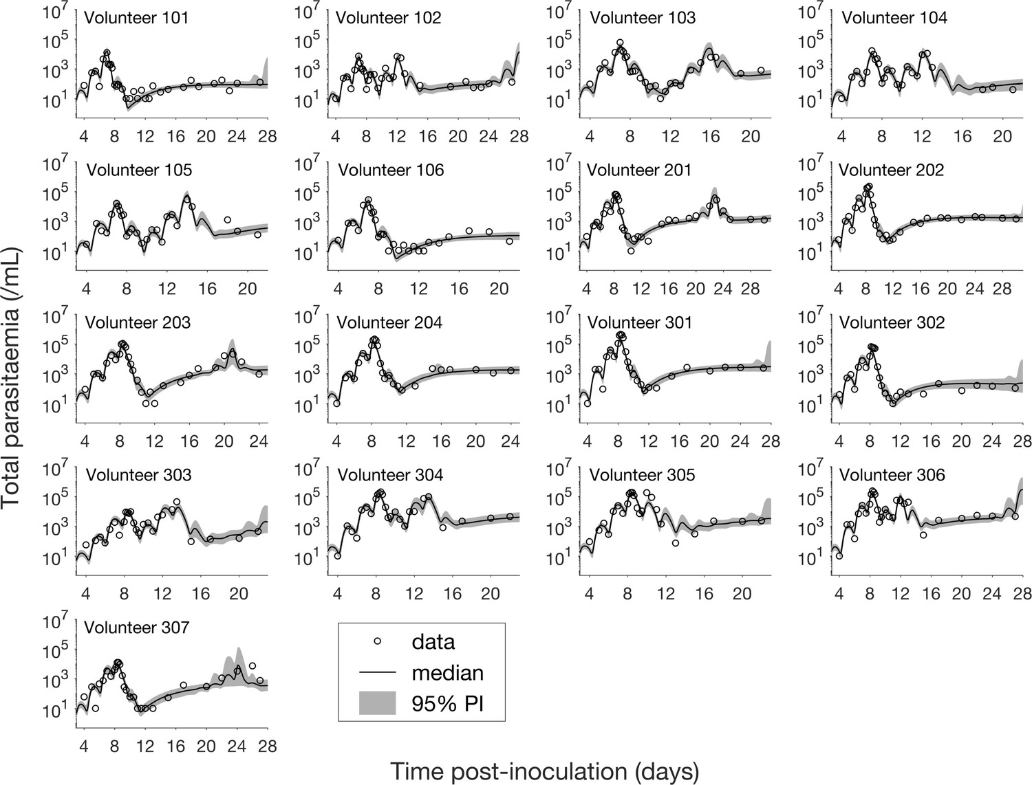
Results of model fitting for all 17 volunteers.

Data are presented by circles. The median of posterior predictions (solid line) and 95% prediction interval (PI, shaded area) are generated by 5000 model simulations based on 5000 samples from the posterior parameter distribution as described in the Materials and methods. The histograms showing the posterior distributions of population mean and standard deviation hyperparameters are given in Figure 1—figure supplements 1 and 2. The posterior distribution of each model parameter (see the Materials and methods) for individual volunteers are given in Figure 1—figure supplements 3–14 Posterior distributions for some biological parameters are given in Figure 1—figure supplement 15, which are generated based on the posterior samples of population mean parameters (see the Materials and methods) and will be used to support the results in Table 1 shown later. The source data and computer code with instructions of implementation to generate Figure 1 and Figure 1—figure supplements 1–15 are fully publicly available at https://doi.org/10.26188/5cde4c26c8201.

https://doi.org/10.7554/eLife.49058.002

Figure 1—figure supplement 1

Download asset Open asset

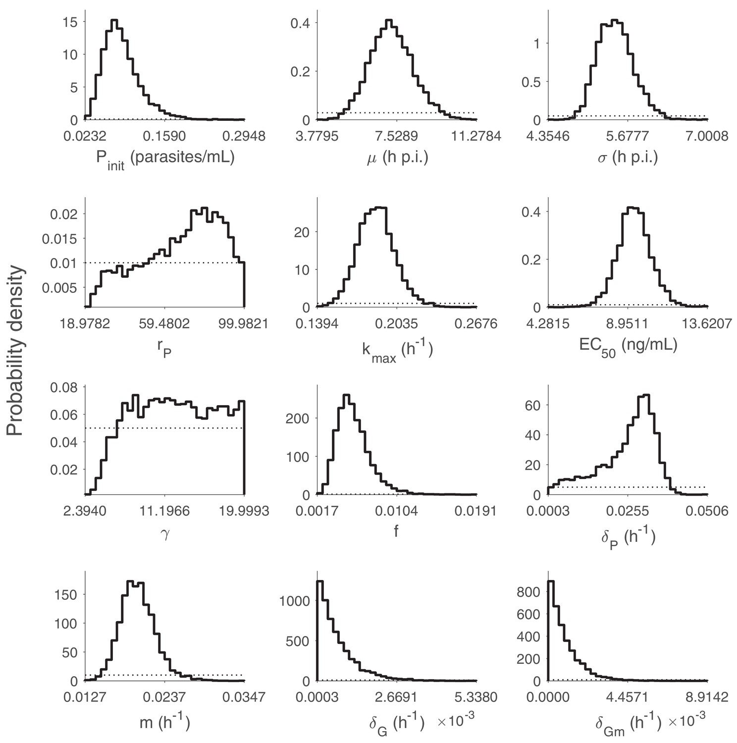
Marginal posterior distributions for the 12 population mean parameters (hyperparameters).

5000 samples are used to generate the distributions. The dashed curves indicate the uniform prior distributions. p.i.: post-inoculation. Note that the y-axis is probability density instead of number of samples. Relevant details of the hyperparameters are provided in the Materials and methods in the main text.

https://doi.org/10.7554/eLife.49058.003

Figure 1—figure supplement 2

Download asset Open asset

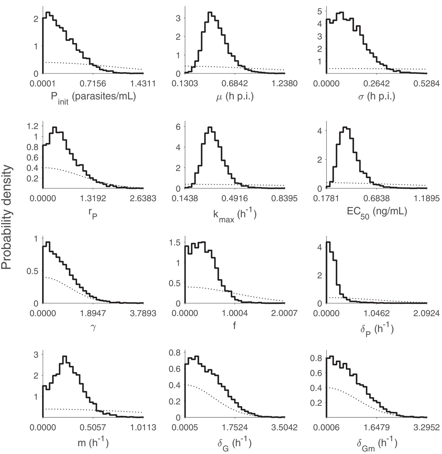
Marginal posterior distributions for the 12 population SD parameters (hyperparameters).

5000 samples are used to generate the distributions. The dashed curves indicate the half-normal prior distributions. p.i.: post-inoculation. Note that the y-axis is probability density instead of number of samples. Relevant details of the hyperparameters are provided in the Materials and methods in the main text.

https://doi.org/10.7554/eLife.49058.004

Figure 1—figure supplement 3

Download asset Open asset

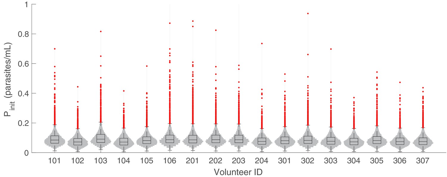
The marginal posterior distributions of the individual parameter of $P_{i n i t}$ (inoculation size) for all 17 volunteers.

The violin plots (gray area) show the distributions of 5000 posterior samples. Box plots show the 25%, 50% (median) and 75% quantiles with outliers indicated by red dots. Relevant details of the individual parameter are provided in the Materials and methods in the main text.

https://doi.org/10.7554/eLife.49058.005

Figure 1—figure supplement 4

Download asset Open asset

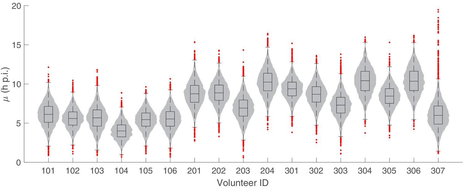
The marginal posterior distributions of the individual parameter of µ (mean of the initial parasite age distribution) for all 17 volunteers.

The violin plots (gray area) show the distributions of 5000 posterior samples. Box plots show the 25%, 50% (median) and 75% quantiles with outliers indicated by red dots. Relevant details of the individual parameter are provided in the Materials and methods in the main text.

https://doi.org/10.7554/eLife.49058.006

Figure 1—figure supplement 5

Download asset Open asset

The marginal posterior distributions of the individual parameter of $σ$ (Standard deviation of the initial parasite age distribution) for all 17 volunteers.

The violin plots (gray area) show the distributions of 5000 posterior samples. Box plots show the 25%, 50% (median) and 75% quantiles with outliers indicated by red dots. Relevant details of the individual parameter are provided in the Materials and methods in the main text.

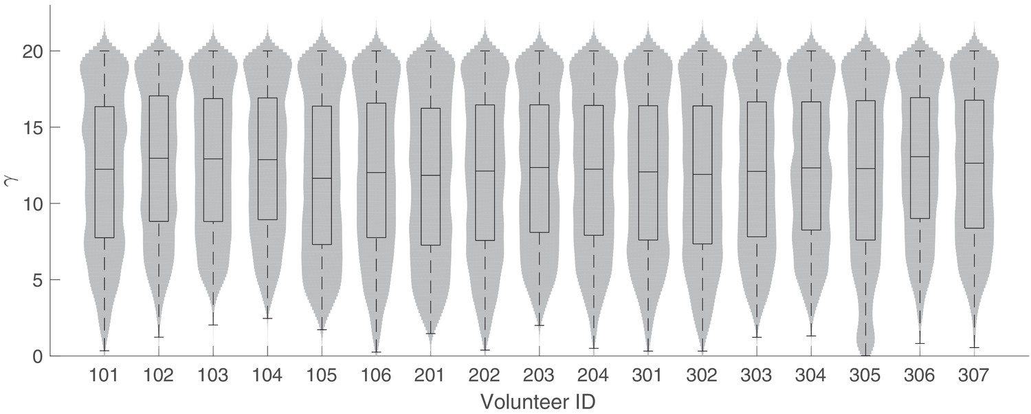
https://doi.org/10.7554/eLife.49058.007

Figure 1—figure supplement 6

Download asset Open asset

The marginal posterior distributions of the individual parameter of $r_{P}$ (parasite replication rate) for all 17 volunteers.

The violin plots (gray area) show the distributions of 5000 posterior samples. Box plots show the 25%, 50% (median) and 75% quantiles with outliers indicated by red dots. Relevant details of the individual parameter are provided in the Materials and methods in the main text.

https://doi.org/10.7554/eLife.49058.008

Figure 1—figure supplement 7

Download asset Open asset

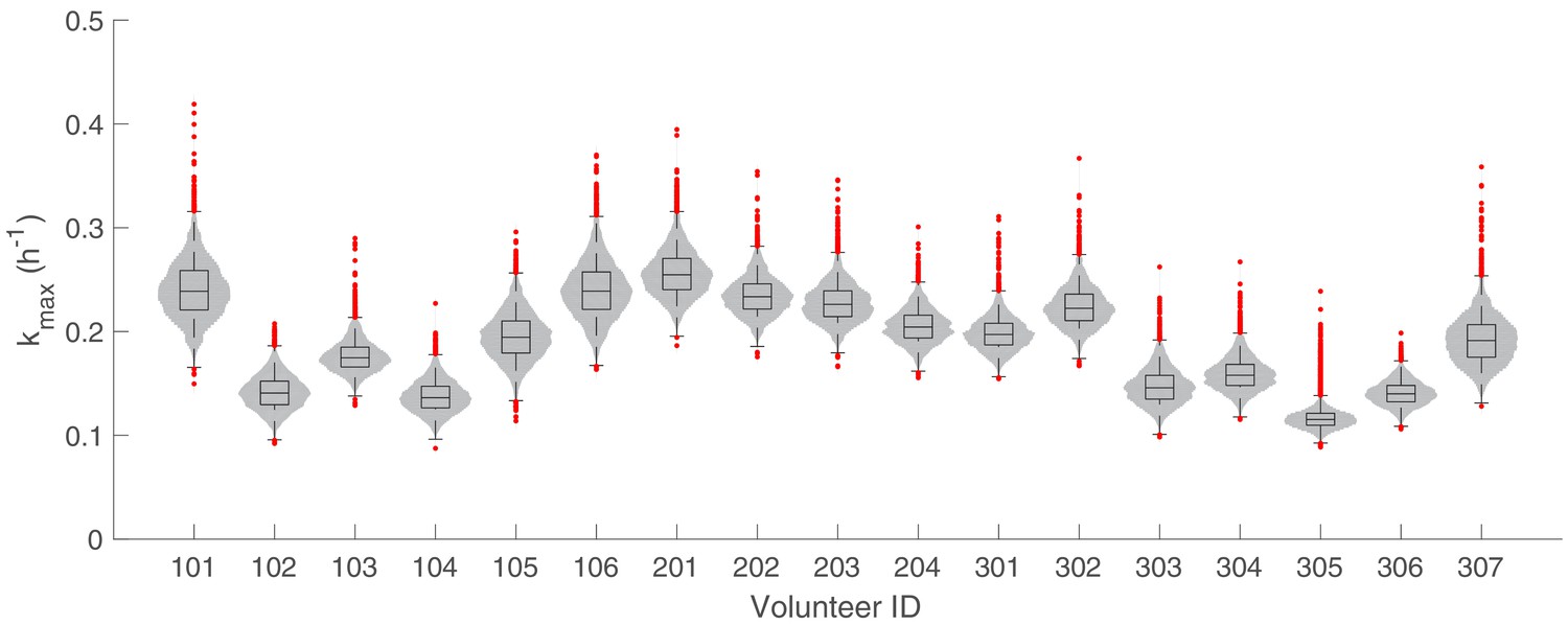
The marginal posterior distributions of the individual parameter of $k_{m a x}$ (maximum rate of parasite killing by PQP) for all 17 volunteers.

The violin plots (gray area) show the distributions of 5000 posterior samples. Box plots show the 25%, 50% (median) and 75% quantiles with outliers indicated by red dots. Relevant details of the individual parameter are provided in the Materials and methods in the main text.

https://doi.org/10.7554/eLife.49058.009

Figure 1—figure supplement 8

Download asset Open asset

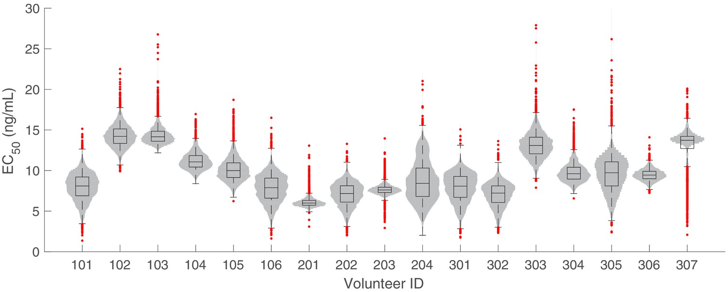
The marginal posterior distributions of the individual parameter of ${E C}_{50}$ (half-maximum effective PQP concentration) for all 17 volunteers.

The violin plots (gray area) show the distributions of 5000 posterior samples. Box plots show the 25%, 50% (median) and 75% quantiles with outliers indicated by red dots. Relevant details of the individual parameter are provided in the Materials and methods in the main text.

https://doi.org/10.7554/eLife.49058.010

Figure 1—figure supplement 9

Download asset Open asset

The marginal posterior distributions of the individual parameter of $γ$ (Hill coefficient for PQP) for all 17 volunteers.

The violin plots (gray area) show the distributions of 5000 posterior samples. Box plots show the 25%, 50% (median) and 75% quantiles with outliers indicated by red dots. Relevant details of the individual parameter are provided in the Materials and methods in the main text.

https://doi.org/10.7554/eLife.49058.011

Figure 1—figure supplement 10

Download asset Open asset

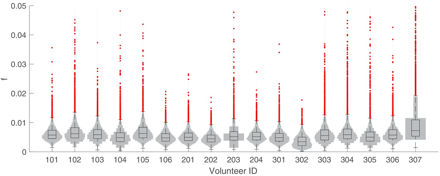
The marginal posterior distributions of the individual parameter of $f$ (sexual commitment rate; not converted to percentage) for all 17 volunteers.

The violin plots (gray area) show the distributions of 5000 posterior samples. Box plots show the 25%, 50% (median) and 75% quantiles with outliers indicated by red dots. Relevant details of the individual parameter are provided in the Materials and methods in the main text.

https://doi.org/10.7554/eLife.49058.012

Figure 1—figure supplement 11

Download asset Open asset

The marginal posterior distributions of the individual parameter of $δ_{P}$ (death rate of asexual and sexual parasites) for all 17 volunteers.

The violin plots (gray area) show the distributions of 5000 posterior samples. Box plots show the 25%, 50% (median) and 75% quantiles with outliers indicated by red dots. Relevant details of the individual parameter are provided in the Materials and methods in the main text.

https://doi.org/10.7554/eLife.49058.013

Figure 1—figure supplement 12

Download asset Open asset

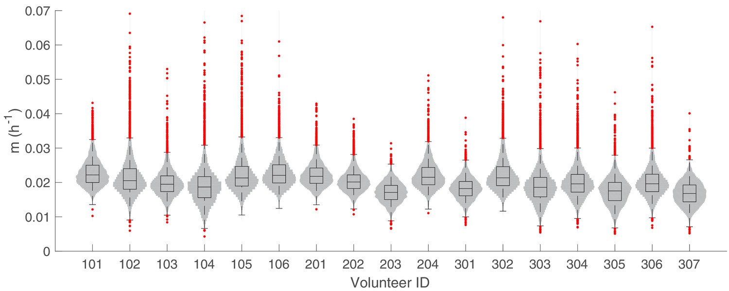
The marginal posterior distributions of the individual parameter of $m$ (maturation rate of gametocytes) for all 17 volunteers.

The violin plots (gray area) show the distributions of 5000 posterior samples. Box plots show the 25%, 50% (median) and 75% quantiles with outliers indicated by red dots. Relevant details of the individual parameter are provided in the Materials and methods in the main text.

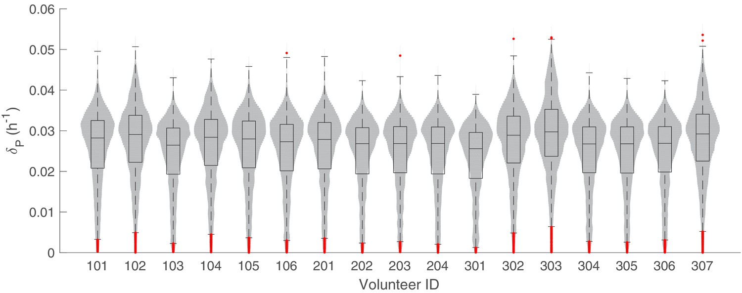
https://doi.org/10.7554/eLife.49058.014

Figure 1—figure supplement 13

Download asset Open asset

The marginal posterior distributions of the individual parameter of $δ_{G}$ (death rate of sequestered gametocytes) for all 17 volunteers.

The violin plots (gray area) show the distributions of 5000 posterior samples. Box plots show the 25%, 50% (median) and 75% quantiles with outliers indicated by red dots. Relevant details of the individual parameter are provided in the Materials and methods in the main text.

https://doi.org/10.7554/eLife.49058.015

Figure 1—figure supplement 14

Download asset Open asset

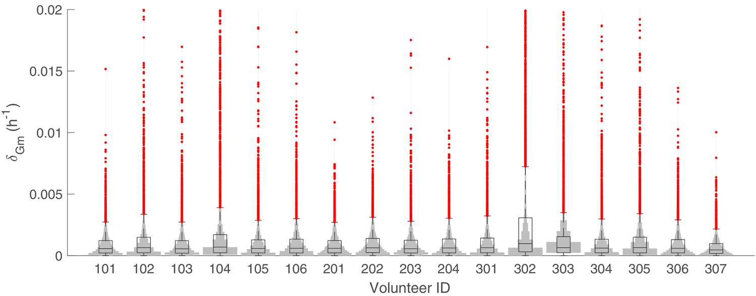
The marginal posterior distributions of the individual parameter of $δ_{G m}$ (death rate of circulating gametocytes) for all 17 volunteers.

The violin plots (gray area) show the distributions of 5000 posterior samples. Box plots show the 25%, 50% (median) and 75% quantiles with outliers indicated by red dots. Relevant details of the individual parameter are provided in the Materials and methods in the main text.

https://doi.org/10.7554/eLife.49058.016

Figure 1—figure supplement 15

Download asset Open asset

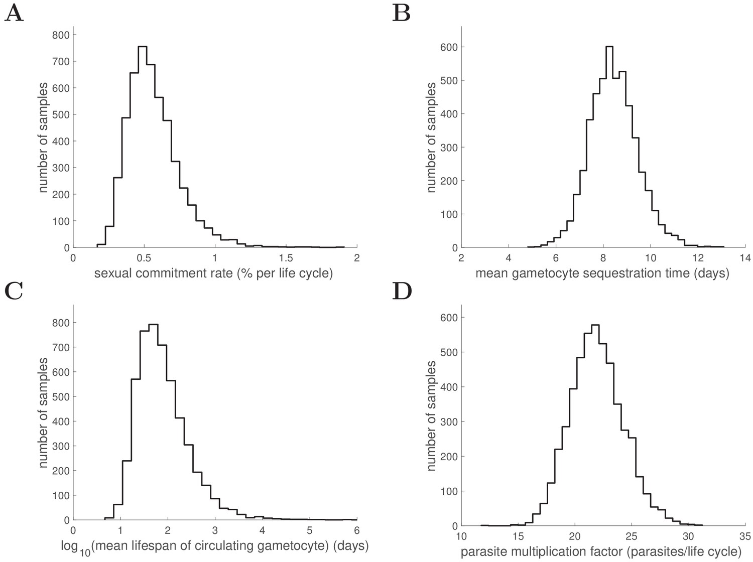
Marginal posterior distributions of some key biological parameters.

5000 samples from the posterior parameter distribution are used to generate the figures. Full details about the definitions and expressions of those biological parameters are provided in the Materials and methods in the main text. Note that a logarithm is taken for the mean lifespan of circulating gametocyte for a better visualisation of the distribution.

https://doi.org/10.7554/eLife.49058.017

Figure 2

Download asset Open asset

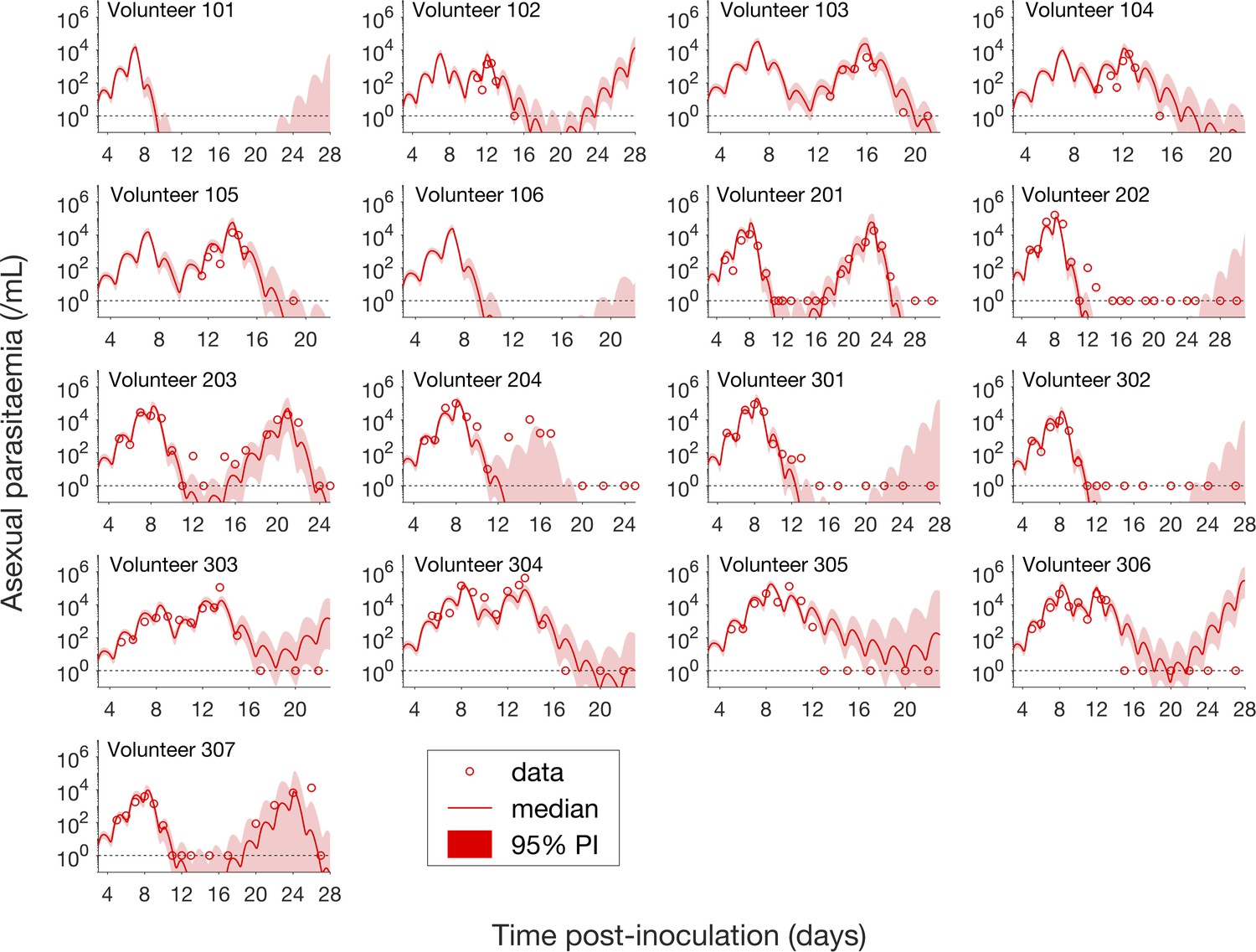
Comparison of model predictions and clinical data for the asexual parasitemia for all 17 volunteers.

Data are presented by circles. The median of posterior predictions (solid curve) and 95% PI (shaded area) are generated by 5000 model simulations based on 5000 samples from the posterior parameter distribution as described in the Materials and methods. The data points with one parasite/mL (i.e., those points which lie on the dotted line) indicate measurements for which no parasites were detected. No data are available for Volunteer 101 and 106 to validate the model predictions. The source data and computer code with instructions of implementation to generate Figure 2 are fully publicly available at https://doi.org/10.26188/5cde4c26c8201.

https://doi.org/10.7554/eLife.49058.019

Figure 3

Download asset Open asset

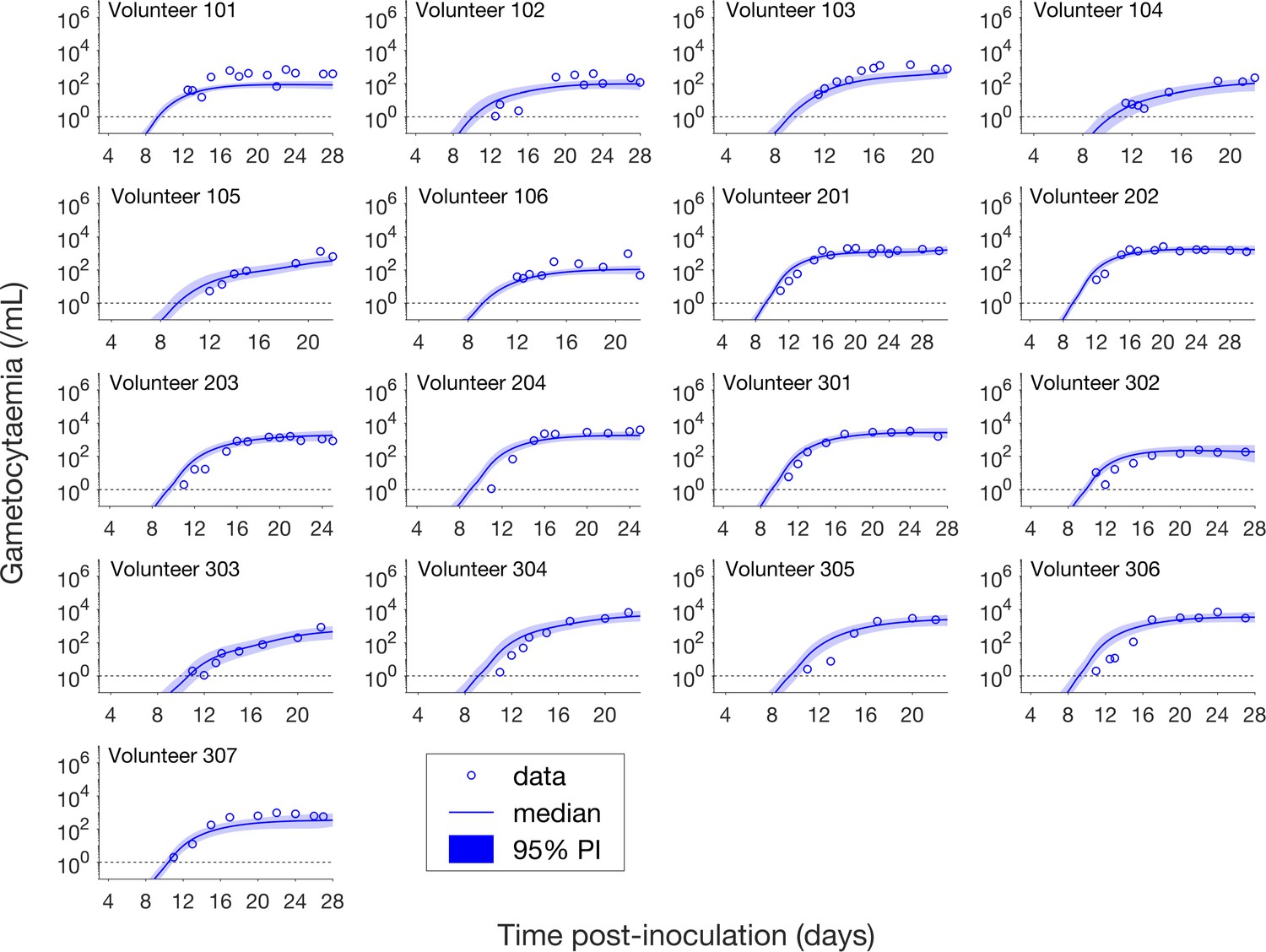
Comparison of model predictions and clinical data for the gametocytemia for all 17 volunteers.

Data are presented by circles. The median of posterior predictions (solid curve) and 95% PI (shaded area) are generated by 5000 model simulations based on 5000 samples from the posterior parameter distribution as described in the Materials and methods. The data points with one parasite/mL (i.e. those points which lie on the dotted line) indicate measurements for which no parasites were detected. The source data and computer code with instructions of implementation to generate Figure 3 are fully publicly available at https://doi.org/10.26188/5cde4c26c8201.

https://doi.org/10.7554/eLife.49058.020

Figure 4

Download asset Open asset

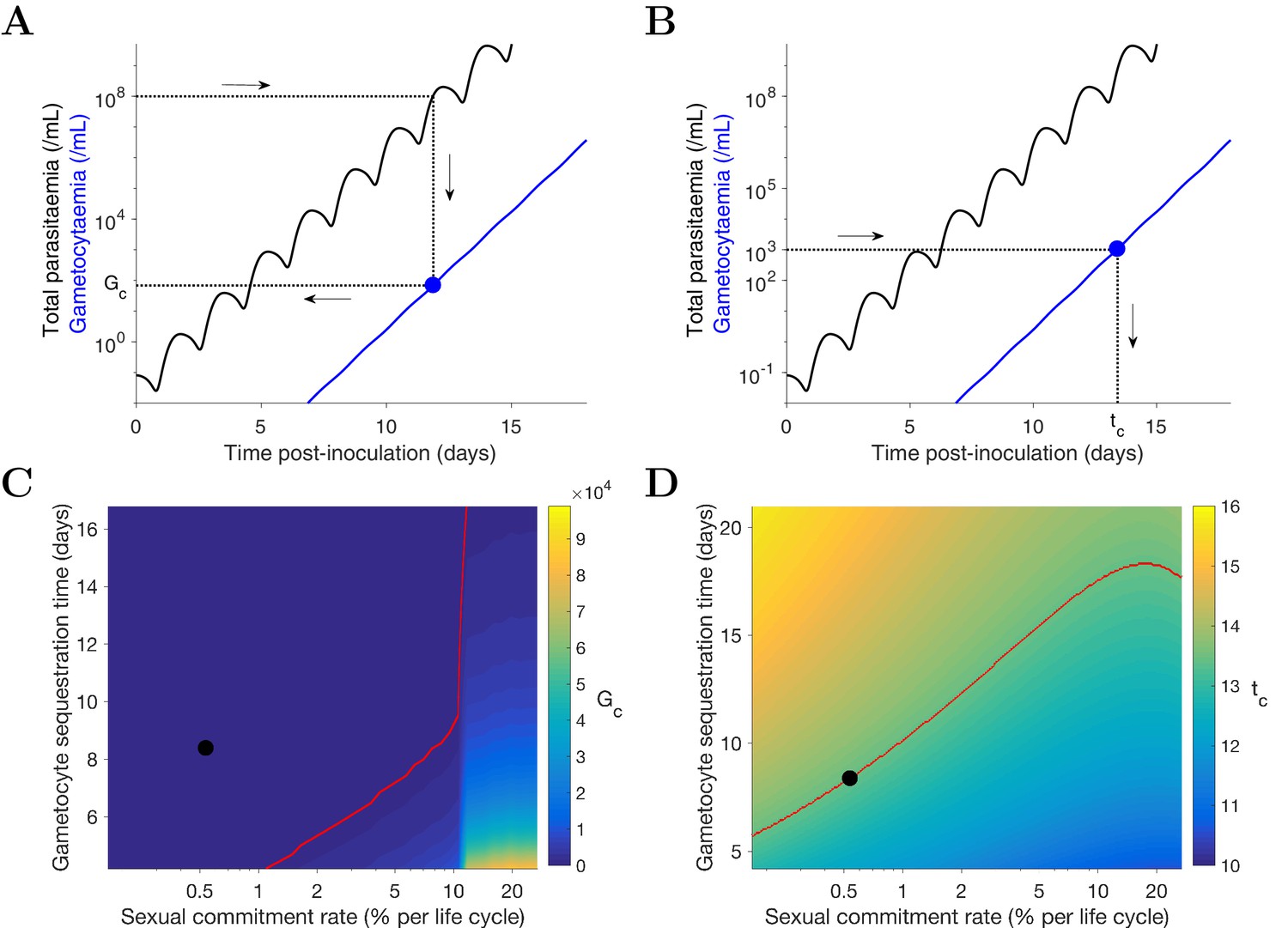
Simulation of two scenarios predicting the dependence of human-to-mosquito transmissibility on the sexual commitment rate and gametocyte sequestration time.

(A) illustration of the first scenario: predicting the critical gametocytemia level (indicated by G_c) at the time when the total parasitemia reaches 10⁸ parasites/mL. (B) illustration of the second scenario: predicting the non-infectious period (indicated by t_c), which is defined to be time from inoculation of infected red blood cells to the time when the gametocytemia reaches 10³ parasites/mL (a threshold below which human-to-mosquito transmission was not observed [Collins et al., 2018]). (**C and D**) Heatmaps showing the dependence of the critical gametocytemia G_c and the non-infectious period t_c on the sexual commitment rate and gametocyte sequestration time. The black dots represent the value obtained by simulating the gametocyte dynamics model using the median estimates of the posterior samples of the population mean parameters as described in the Materials and methods. The red curve in C is the level curve for G_c = 10³ parasites/mL. The red curve in D is the level curve for t_c = 13.42 days which is the non-infectious period obtained by model simulation using the posterior estimates of the population mean parameters. The source data and computer code with instruction of implementation to generate Figure 4 are fully publicly available at https://doi.org/10.26188/5cde4c26c8201.

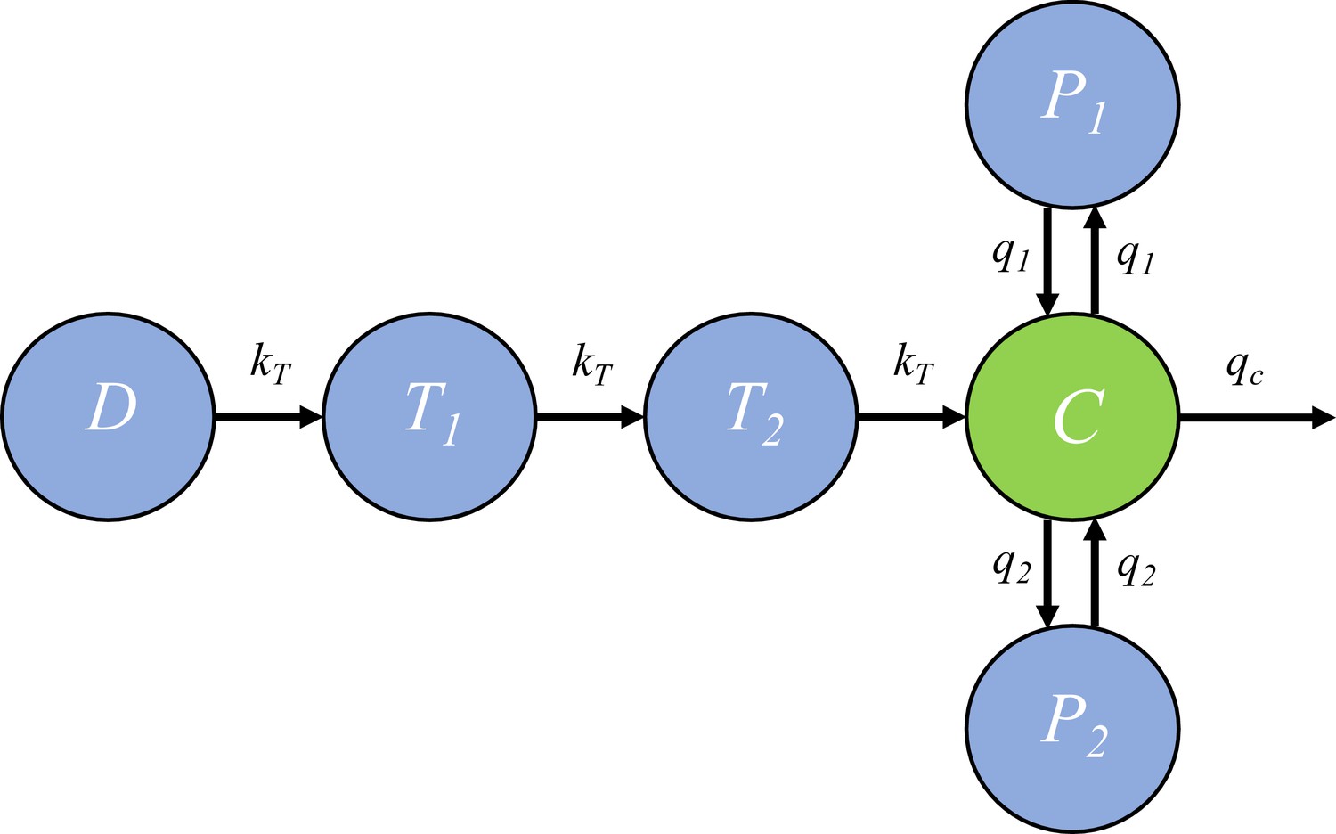
https://doi.org/10.7554/eLife.49058.021

Figure 5

Download asset Open asset

Schematic diagram showing the model compartments and transitions.

The model is comprised of three parts describing three populations of parasites: asexual parasites ( $P (a, t)$ ), sexually committed parasites ( $P_{G} (a, t)$ ) and gametocytes ( $G (t)$ ). P and P_G are functions of asexual parasite age $a$ and time $t$ . Square compartments in the inner loop represent the asexual parasite population which follows a cycle of maturation and replication every $a_{L}$ hours. Sexual commitment occurs from age $a_{s}$ and a fraction of asexual parasites become sexually committed (the bigger square compartments in the outer loop) and eventually enter the development of stage I–V gametocytes (G₁–G₅). The compartments with a dashed boundary are sequestered to tissues and thus not measurable in a blood smear. The notation for each compartment is consistent with those in the model equations and is explained in the main text.

https://doi.org/10.7554/eLife.49058.022

Figure 6 with 1 supplement

Download asset Open asset

The pharmacokinetic model of piperaquine (PQP).

The model is a three-compartment disposition model with two transit compartments for absorption. State D represents the dose of PQP. T₁ and T₂ represent the two transit compartments. C is the central compartment and PQP concentration in this compartment was measured (which are shown in Figure 6—figure supplement 1). P₁ and P₂ represent two peripheral compartments. *k_T, q₁, q₂* and *q_c* are the rates of flow into or out of compartments.

https://doi.org/10.7554/eLife.49058.024

Figure 6—figure supplement 1

Download asset Open asset

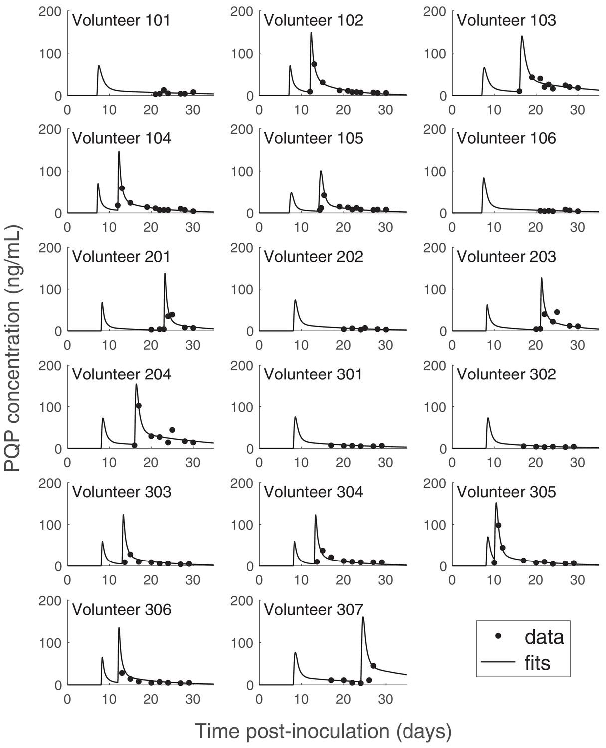
PK data and optimized PK curves (the ‘fits’) of piperaquine (PQP) concentration for all volunteers.

The details of the optimization approach are provided in the Materials and methods in the main text and Appendix 1. Some volunteers have two peaks of PQP concentrations because they had recrudescent asexual parasitemia (see Figure 1 in the main text) and were treated with a second dose of 960 mg PQP. The source data and computer code with instructions of implementation to generate Figure 6—figure supplement 1 are fully publicly available at https://doi.org/10.26188/5cde4c26c8201.

https://doi.org/10.7554/eLife.49058.025

Tables

Table 1

Estimates of some key biological parameters and comparison with the literature.

The estimates of the biological parameters (middle column) are shown as the median and 95% credible interval (CI) of the marginal posterior parameter distribution (Figure 1—figure supplement 15). Estimates from the literature (third column) are shown in the format of either ‘mean estimate (95% confidence interval)’ or ‘mean estimate [minimum – maximum estimate]’ or simply ‘a low estimate – a high estimate’. Note some quoted estimates are from either in vivo or in vitro studies of P. falciparum. The source data and computer code with instructions of implementation to generate our model estimates (middle column) in Table 1 are fully publicly available at https://doi.org/10.26188/5cde4c26c8201.

https://doi.org/10.7554/eLife.49058.018

Biological parameters (unit)	Median estimate (95% CI)	Estimates in the literature
Sexual commitment rate (%/asexual replication cycle)	0.54 (0.30–1.00)	11 (6.2–15.8) (Filarsky et al., 2018) (in vitro) 0.64 [0.027–13.5] (Eichner et al., 2001) (in vivo)
Gametocyte sequestration time (days)	8.39 (6.54–10.59)	7.4 [4 – 12] (Eichner et al., 2001) (in vivo)
Circulating gametocyte lifespan (days)	63.5 (12.7–1513.9)	16–32 (Gebru et al., 2017) (in vitro) 6.4 [1.3–22.2] (Eichner et al., 2001) (in vivo)
Parasite multiplication factor (per asexual replication cycle)	21.8 (17.6–26.9)	10–33 (Wockner et al., 2017) (in vivo) 16.4 (15.1–17.8)^a (in vivo)

^a JS McCarthy, personal communication, May 2019.

Table 2

Details of the gametocyte dynamics model parameters.

The table includes the unit, description and prior distribution for each model parameter. For the uniform prior distributions (U), the lower bounds are non-negative based on the definitions of the model parameters and the upper bounds for the prior distributions were chosen to be sufficiently wide in order to accommodate all biologically plausible values from the literature (Zaloumis et al., 2012). We assumed parasites younger than 25h are circulating and thus fix $a_{s}$ to be 25h. For 3D7 strain, the asexual replication cycle is approximately 39–45h (based on in vitro estimates [Duffy and Avery, 2017] and personal communication [JS McCarthy, personal communication, May 2019]) and we fix $a_{L}$ to be 42h.

https://doi.org/10.7554/eLife.49058.023

Parameter	Unit	Description	Prior distribution
$P_{i n i t}$	parasites/mL	inoculation size	U(0, 10)
$μ$	h	mean of the initial parasite age distribution	U(0, 35)
$σ$	h	SD of the initial parasite age distribution	U(0, 20)
$r_{P}$	(unitless)	parasite replication rate	U(0, 100)
$k_{m a x}$	h⁻¹	maximum rate of parasite killing by PQP	U(0, 1)
$E C_{50}$	ng/mL	half-maximum effective PQP concentration	U(1, 100)
$γ$	(unitless)	Hill coefficient for PQP	U(0, 20)
$f$	(unitless)	the fraction of parasites entering sexual development per asexual replication cycle	U(0, 1)
$δ_{P}$	h⁻¹	death rate of asexual and sexual parasites	U(0, 0.2)
$m$	h⁻¹	maturation rate of gametocytes	U(0, 0.1)
$δ_{G}$	h⁻¹	death rate of sequestered gametocytes	U(0, 0.1)
$δ_{G m}$	h⁻¹	death rate of circulating gametocytes	U(0, 0.1)
$a_{s}$	h	sequestration age of asexual parasites	fixed to be 25
$a_{L}$	h	length of life cycle of asexual parasites	fixed to be 42

SD: standard deviation; h: hour.

Appendix 1—table 1

Parameter values used to generate the optimized PK curves for all 17 volunteers.

The units of the model parameters are given in the parentheses. The optimized PK curves are shown in Figure 6—figure supplement 1.

https://doi.org/10.7554/eLife.49058.028

PK parameter (unit)	k_T(h^-1)	q_c(L/h)	V_c(L)	q₁(L/h)	V₁(L)	q₂(L/h)	v₂(L)
Volunteer 101	1/2.43	53.7	831	2240	3958	118	17177
Volunteer 102	1/2.32	123.4	582	849	3985	163	10355
Volunteer 103	1/3.07	61.3	756	2686	3910	127	14346
Volunteer 104	1/2.32	134.7	488	746	3986	190	15007
Volunteer 105	1/3.25	160	1342	5034	3986	190	17546
Volunteer 106	1/2.40	60.7	667	2992	3043	123	16374
Volunteer 201	1/2.32	160	469	746	3986	190	15557
Volunteer 202	1/2.79	71.4	804	2020	3010	149	13300
Volunteer 203	1/2.32	141.9	1243	803	3973	190	11825
Volunteer 204	1/2.32	63.3	895	2169	3327	165	16205
Volunteer 301	1/2.79	61.4	804	2020	3010	149	13300
Volunteer 302	1/2.79	81.4	804	2020	3010	149	13300
Volunteer 303	1/2.45	159.4	1332	779	3970	190	17355
Volunteer 304	1/2.48	158.9	1339	762	3981	190	17290
Volunteer 305	1/2.53	120.9	1152	1905	2979	123	13896
Volunteer 306	1/2.32	158.8	870	761	3983	190	17488
Volunteer 307	1/2.79	51.4	804	2020	3010	149	13300

Additional files

Transparent reporting form: https://doi.org/10.7554/eLife.49058.026
Download elife-49058-transrepform-v1.pdf

Download links

A two-part list of links to download the article, or parts of the article, in various formats.

Downloads (link to download the article as PDF)

Open citations (links to open the citations from this article in various online reference manager services)

Mendeley

Cite this article (links to download the citations from this article in formats compatible with various reference manager tools)

Pengxing Cao
Katharine A Collins
Sophie Zaloumis
Thanaporn Wattanakul
Joel Tarning
Julie A Simpson
James McCarthy
James M McCaw

(2019)

Modeling the dynamics of Plasmodium falciparum gametocytes in humans during malaria infection

eLife 8:e49058.

https://doi.org/10.7554/eLife.49058

Share this article

Cite this article

Results of model fitting for all 17 volunteers.

Marginal posterior distributions for the 12 population mean parameters (hyperparameters).

Marginal posterior distributions for the 12 population SD parameters (hyperparameters).

The marginal posterior distributions of the individual parameter of Pinit (inoculation size) for all 17 volunteers.

The marginal posterior distributions of the individual parameter of µ (mean of the initial parasite age distribution) for all 17 volunteers.

The marginal posterior distributions of the individual parameter of σ (Standard deviation of the initial parasite age distribution) for all 17 volunteers.

The marginal posterior distributions of the individual parameter of rP (parasite replication rate) for all 17 volunteers.

The marginal posterior distributions of the individual parameter of kmax (maximum rate of parasite killing by PQP) for all 17 volunteers.

The marginal posterior distributions of the individual parameter of EC50 (half-maximum effective PQP concentration) for all 17 volunteers.

The marginal posterior distributions of the individual parameter of γ (Hill coefficient for PQP) for all 17 volunteers.

The marginal posterior distributions of the individual parameter of f (sexual commitment rate; not converted to percentage) for all 17 volunteers.

The marginal posterior distributions of the individual parameter of δP (death rate of asexual and sexual parasites) for all 17 volunteers.

The marginal posterior distributions of the individual parameter of m (maturation rate of gametocytes) for all 17 volunteers.

The marginal posterior distributions of the individual parameter of δG (death rate of sequestered gametocytes) for all 17 volunteers.

The marginal posterior distributions of the individual parameter of δGm (death rate of circulating gametocytes) for all 17 volunteers.

Marginal posterior distributions of some key biological parameters.

Comparison of model predictions and clinical data for the asexual parasitemia for all 17 volunteers.

Comparison of model predictions and clinical data for the gametocytemia for all 17 volunteers.

Simulation of two scenarios predicting the dependence of human-to-mosquito transmissibility on the sexual commitment rate and gametocyte sequestration time.

Schematic diagram showing the model compartments and transitions.

The pharmacokinetic model of piperaquine (PQP).

PK data and optimized PK curves (the ‘fits’) of piperaquine (PQP) concentration for all volunteers.

Estimates of some key biological parameters and comparison with the literature.

Details of the gametocyte dynamics model parameters.

Parameter values used to generate the optimized PK curves for all 17 volunteers.

Transparent reporting form

Downloads (link to download the article as PDF)

Open citations (links to open the citations from this article in various online reference manager services)

Cite this article (links to download the citations from this article in formats compatible with various reference manager tools)

The marginal posterior distributions of the individual parameter of $P_{i n i t}$ (inoculation size) for all 17 volunteers.

The marginal posterior distributions of the individual parameter of $σ$ (Standard deviation of the initial parasite age distribution) for all 17 volunteers.

The marginal posterior distributions of the individual parameter of $r_{P}$ (parasite replication rate) for all 17 volunteers.

The marginal posterior distributions of the individual parameter of $k_{m a x}$ (maximum rate of parasite killing by PQP) for all 17 volunteers.

The marginal posterior distributions of the individual parameter of ${E C}_{50}$ (half-maximum effective PQP concentration) for all 17 volunteers.

The marginal posterior distributions of the individual parameter of $γ$ (Hill coefficient for PQP) for all 17 volunteers.

The marginal posterior distributions of the individual parameter of $f$ (sexual commitment rate; not converted to percentage) for all 17 volunteers.

The marginal posterior distributions of the individual parameter of $δ_{P}$ (death rate of asexual and sexual parasites) for all 17 volunteers.

The marginal posterior distributions of the individual parameter of $m$ (maturation rate of gametocytes) for all 17 volunteers.

The marginal posterior distributions of the individual parameter of $δ_{G}$ (death rate of sequestered gametocytes) for all 17 volunteers.

The marginal posterior distributions of the individual parameter of $δ_{G m}$ (death rate of circulating gametocytes) for all 17 volunteers.