From single neurons to behavior in the jellyfish Aurelia aurita
- University of Bonn, Germany
Figures
Figure 1
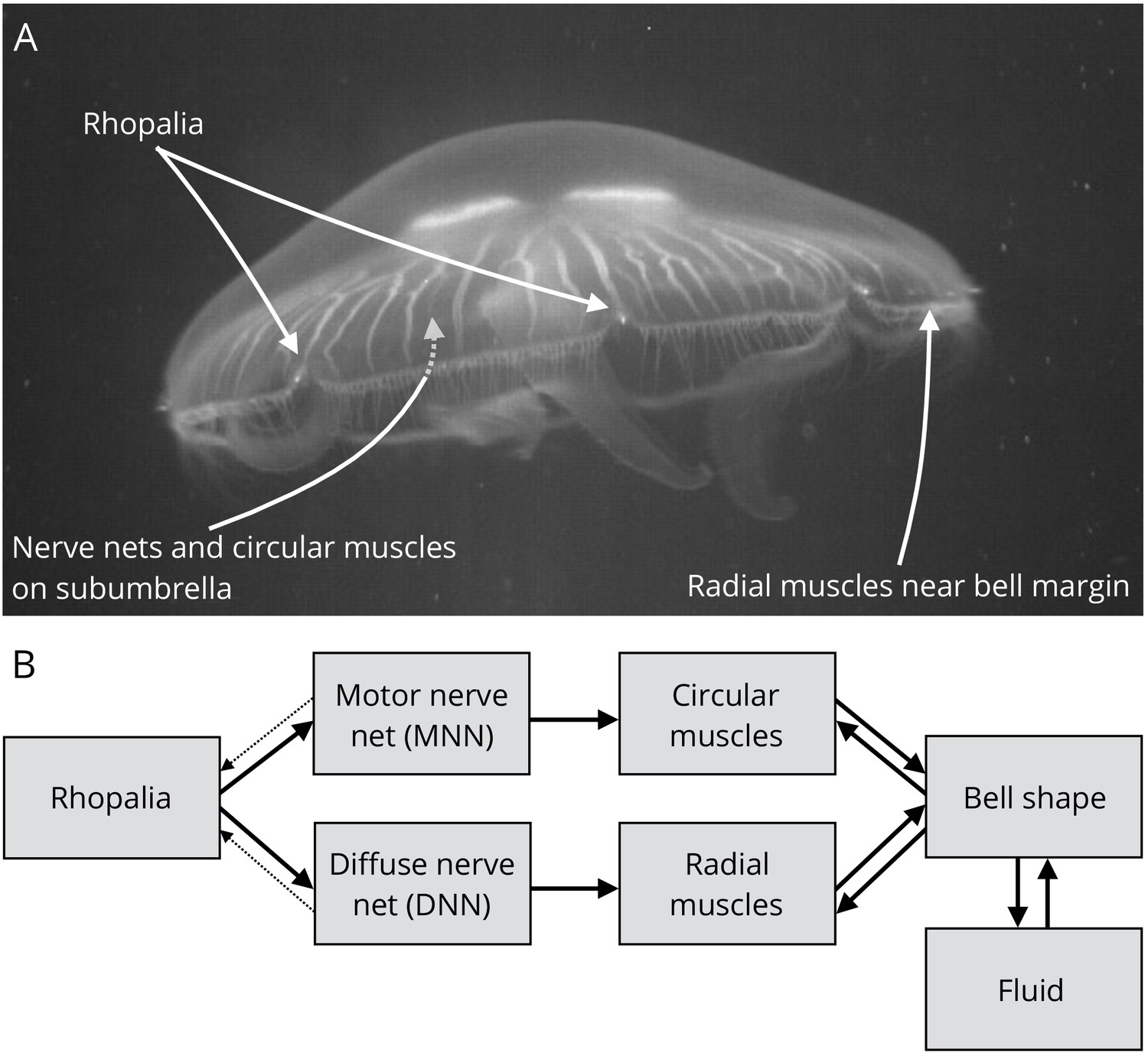
Jellyfish anatomy and schematic overview of our model.
(A) Moon jelly Aurelia aurita in water. The bell is nearly relaxed. Rhopalia are clearly visible as bright spots on wedge-shaped sections of the bell margin. The location of modeled nerve nets and muscles is marked by arrows. (B) Diagram of the jellyfish model components. Rhopalia can be excited by external stimulation. They are connected to both the motor nerve net (MNN) and the separate diffuse nerve net (DNN) on the subumbrella. The MNN selectively innervates the circular muscles, while the DNN selectively innervates the radial ones. The muscles deform the jellyfish bell, which interacts with the surrounding fluid. The muscle forces in turn depend on the bell shape. A putative coupling from MNN and DNN back to the rhopalia (not modeled in this study) is indicated by thin dashed arrows.
Figure 2
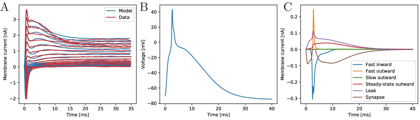
The biophysical model fitted to the voltage-clamp data.
(A) Comparison of our model dynamics with the voltage-clamp data (Anderson, 1989) that was used to fit its current parameters. The model follows the experimentally found traces. (B) Membrane voltage of a neuron that is stimulated by a synaptic EPSC at time zero. The model neuron generates an action potential similar in shape to experimentally observed ones. (C) The disentangled transmembrane currents during an action potential.
Figure 3
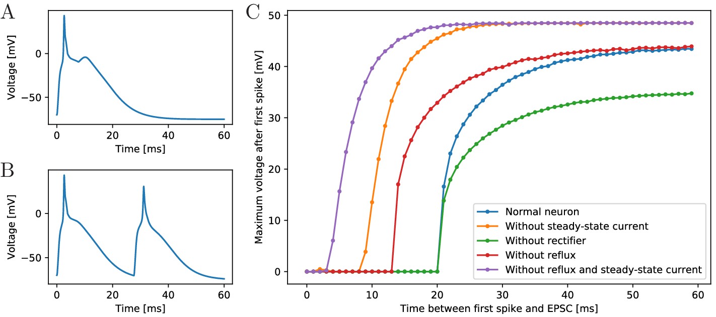
Excitability of an MNN neuron after spiking.
(A,B) Voltage of an example neuron receiving two identical EPSCs (A) 7 ms apart and (B) 25 ms apart. (C) Maximum voltage reached in response to the second EPSC for different time lags between the inputs. The first EPSC always generates a spike. The abscissa displays the time differences between its peak and the onset of the second EPSC. The ordinate displays the highest voltage reached after the end of the first spike, defined as reaching 0 mV from above. A plotted value of 0 mV means that the neuron did not exceed 0 mV after its first spike.
Figure 4

Synaptic density and activity propagation speed in von Mises and uniform MNNs.
(A) Average intersynaptic distance as a function of neuron number in von Mises and uniform MNNs. The dashed line indicates 70 µm (Anderson, 1985). (B) Delay between the spike times of the pacemaker initiating an activation wave and the opposing one, for different MNN neuron numbers. Displayed are results for model jellyfish with 3 cm and 4 cm diameter. The dashed line indicates the experimentally measured average delay of 30 ms between muscle contractions on the initiating and the opposite side of Aurelia aurita (Gemmell et al., 2015); the gray area shows its ±1 std. dev. interval. (C) Delays measured in (B) for the 4 cm jellyfish, plotted against the average number of synapses in MNNs with identical size. Measurement points are averages over 10 MNN realizations; bars indicate one standard deviation.
Figure 5 with 1 supplement
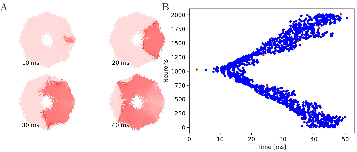
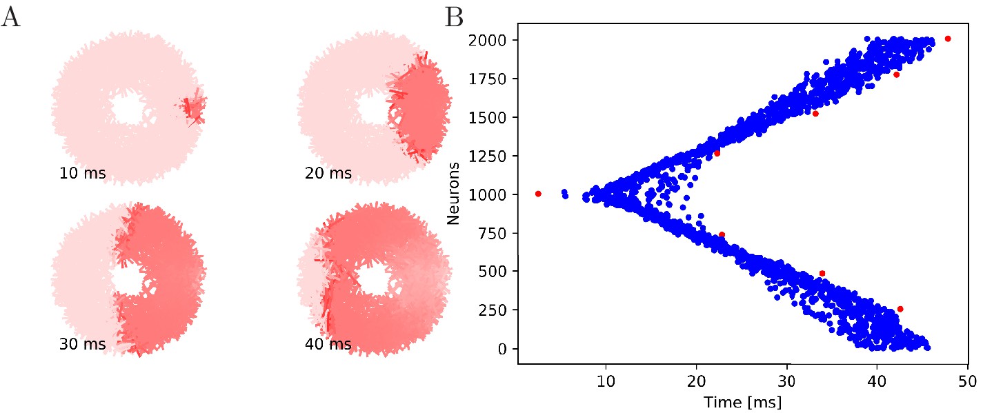
Wave of activation in a von Mises MNN with 2000 neurons.
(A) Activity of each neuron at different times after stimulation of a single pacemaker neuron. Color intensity increases linearly with neuron voltage. (B) Spike times of the same network. Neurons are numbered by their position on the bell. Red dots represent the pacemakers inside one of the eight rhopalia. The neurite orientations are distributed according to location-dependent von Mises distributions.
Figure 5—animation 1
Example animation of Figure 5 (A).
Figure 6
Wave of activation in a uniform MNN with 2000 neurons.
Setup similar to Figure 5, but the neurite orientations are uniformly distributed.
Figure 7 with 1 supplement
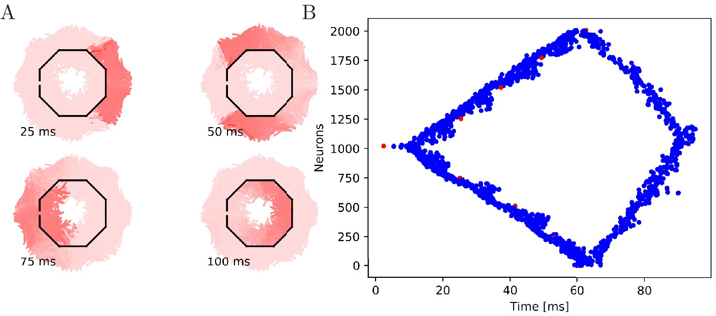
Propagation in a circularly cut von Mises MNN with 2000 neurons.
Setup similar to Figure 5, but black line segments indicate cuts through the nervous system where neurites are severed. Cuts are placed along the outline of an octagon with a small gap through which the signal can propagate to the central neurons.
Figure 7—animation 1
Example animation of Figure 7 (A).
Figure 8 with 1 supplement

Propagation in a radially cut von Mises MNN with 2000 neurons.
Setup similar to Figure 7, but the cuts are placed radially creating a zig-zag patterned bell.
Figure 8—animation 1
Example animation of Figure 8 (A).
Figure 9

Cutting experiments in uniform MNNs with 2000 neurons.
Figure 10 with 2 supplements

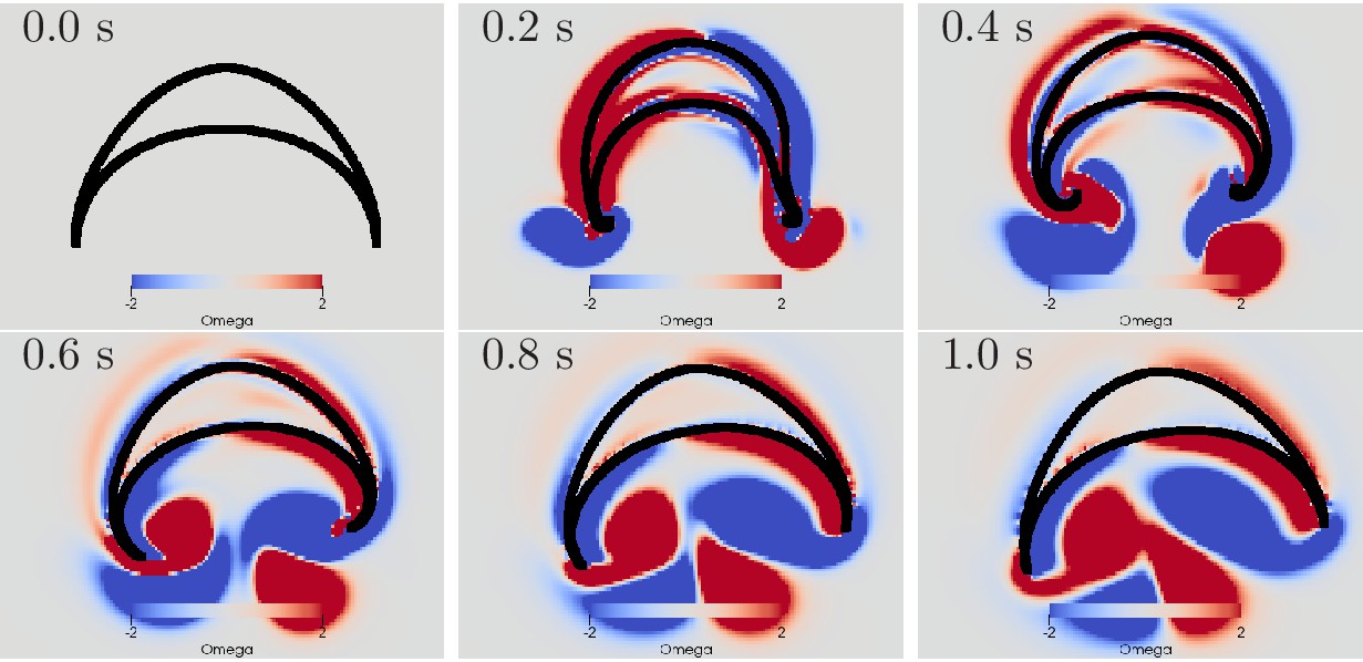
Swimming stroke evoked by a wave of activation in the MNN.
The panels show the dynamics of the bell surface (black) and internal and surrounding media (grey), in steps of 200 ms. Coloring indicates medium vorticity (in ), red a clockwise eddy and blue an anticlockwise one. In this and all following figures, it is the pacemaker on the left hand side of the bell that initiates MNN activation. Further, if not stated otherwise, the MNN has 10,000 neurons.
Figure 10—Animation 1
Animation of the swimming motion.
Figure 10—Animation 2
Animation of both a swimming stroke and the corresponding MNN activation as seen in Figure 5.
Figure 11
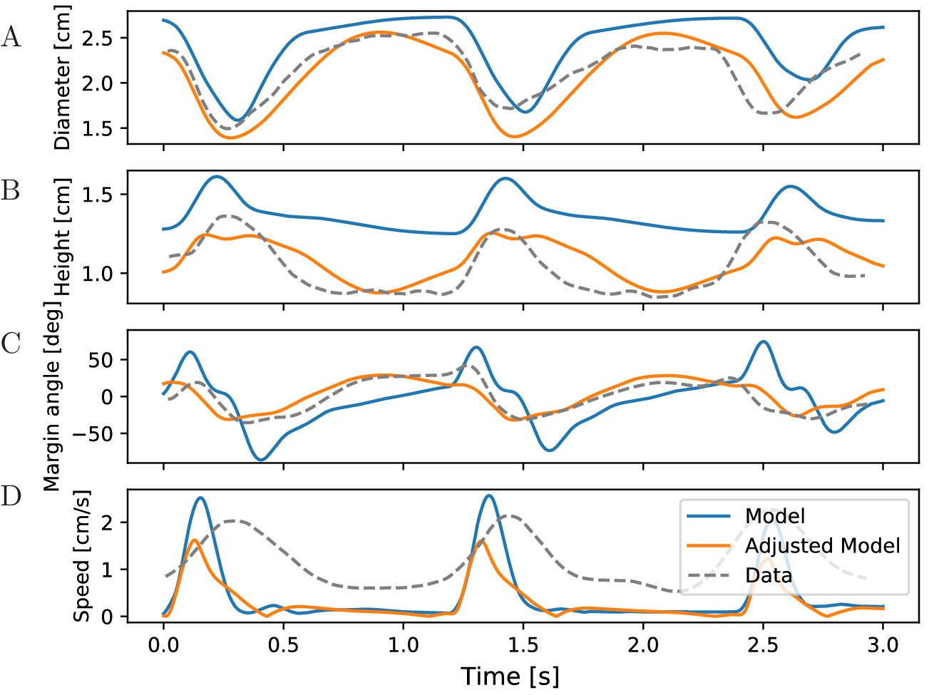
Characteristics of bell shape during swimming.
Dynamics of (A) bell diameter, (B) bell height and (C) the orientation of the margin of the bell relative to the orientation of the bell as a whole, during a sequence of swimming strokes as in Figure 10A, initialized in intervals of 1.2 s. (D) Corresponding speed profile. Shown are models with our standard parameters (blue) and manually adjusted parameters (orange) to match the experimentally found traces (gray) in McHenry and Jed (2003) (Fig. 2 ibid., adapted with permission from Journal of Experimental Biology).
Figure 12
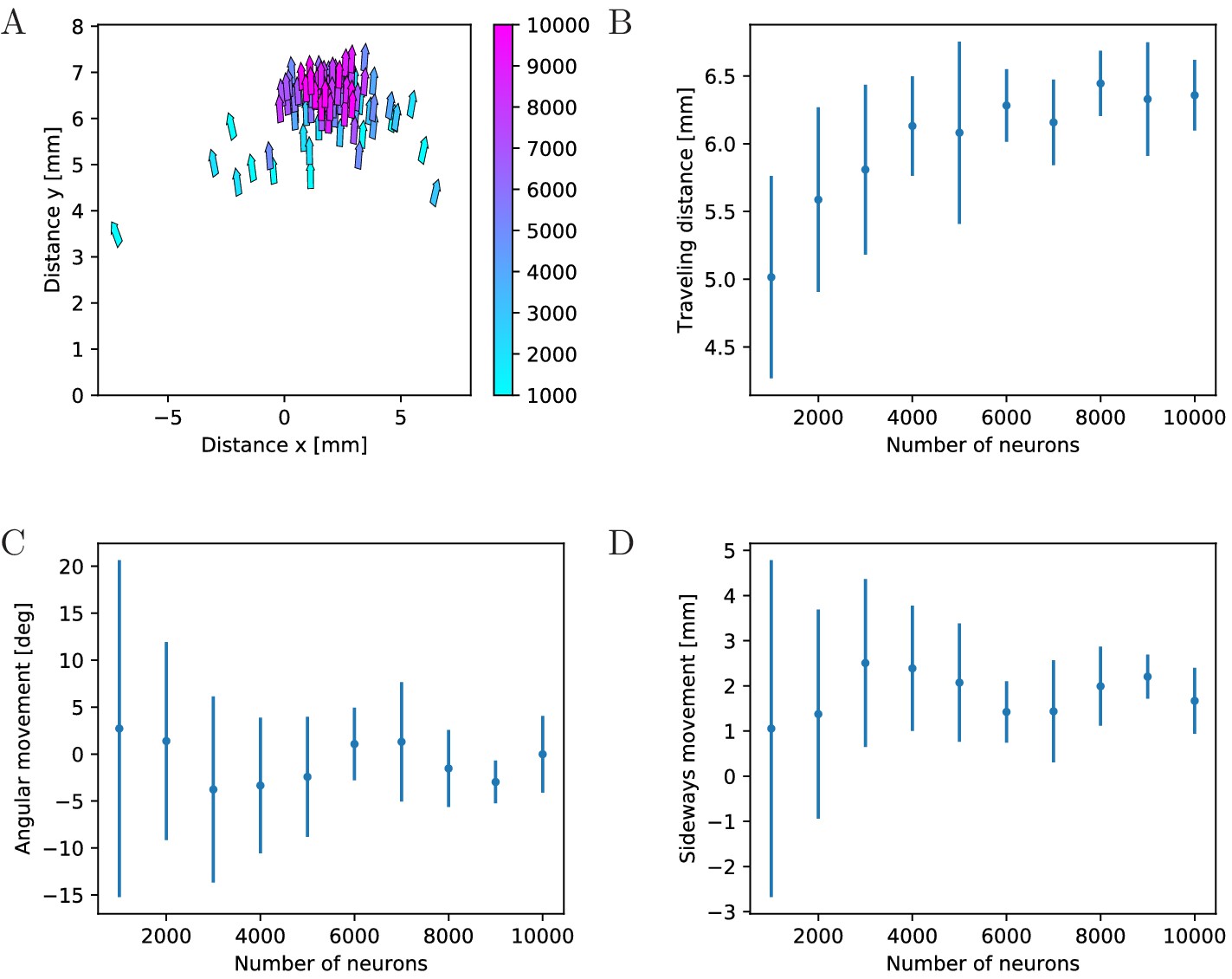
Characteristics of swimming strokes for different MNN sizes.
A shows the distance traveled within a single swimming stroke (origins of arrows) and the orientation after the stroke (direction of arrows) for 100 jellyfish with different MNNs. Color indicates the MNN sizes, which range in 10 steps from 1000 to 10,000. (B, C, D) visualize the dependence of the distributions of swimming characteristics on MNN size. B shows the total distances traveled, C the angular movements (i.e. angular changes in spatial orientation, in degrees) and D the distances moved perpendicularly to the original orientation of the jellyfish. Measurement points are the averages of the 10 jellyfish with MNNs of the same size in A, bars indicate one standard deviation.
Figure 13 with 1 supplement
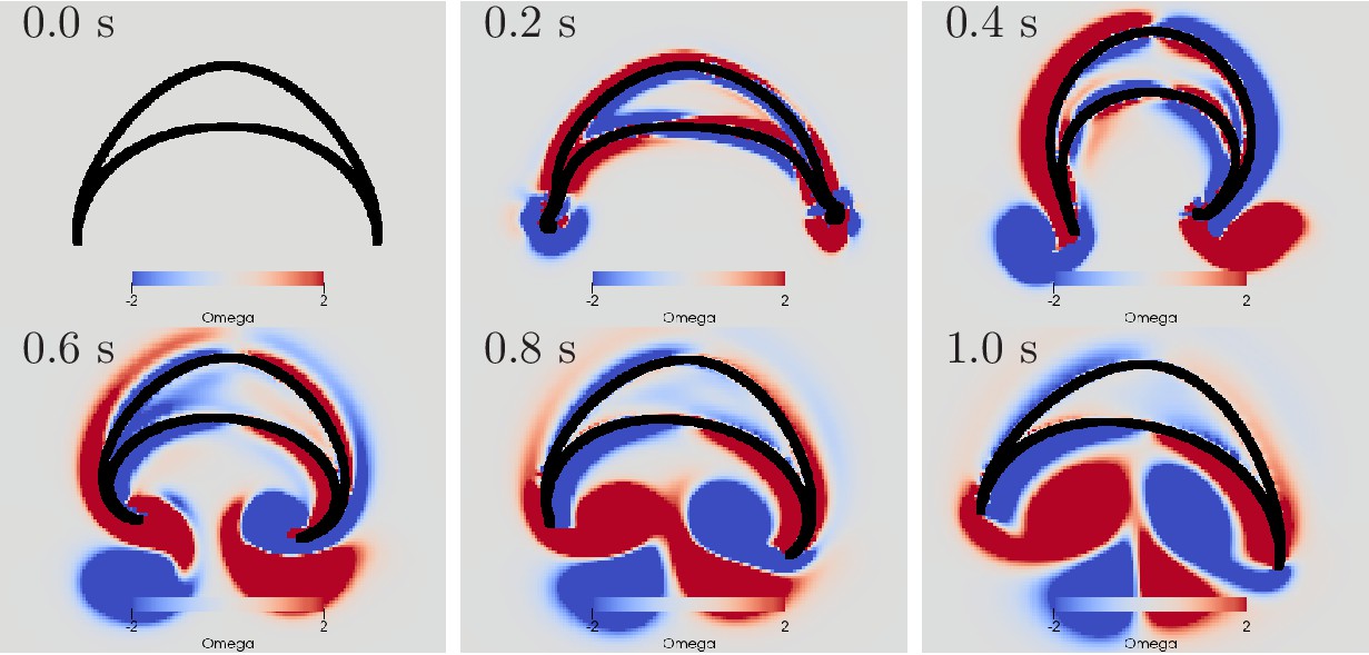
Swimming stroke evoked by simultaneously initiated waves in MNN and DNN.
The activity in the DNN and MNN leads to a simultaneous contraction of the left bell margin and the left bell swim musculature near the margin. The jellyfish therefore turns in the direction of the initiating rhopalium. The DNN has 4000 neurons. MNN and further description are as in Figure 10.
Figure 13—Animation 1
Animation of the swimming motion.
Figure 14

Dependence of turning on the delay between DNN and MNN activation.
(A) Angular movement of model jellyfish versus delay between DNN and MNN activation. The panel displays the angular movement one second after the initiation of the MNN. Turns toward the initiating rhopalium have positive angular movements, while turns away have negative ones. Blue, orange, green and red coloring indicates DNN sizes of 4000, 7000, 10,000 and 13,000 neurons. (B) Delay between initiation of DNN activity and its reaching of the opposing side, as a function of the number of DNN neurons (similar to Figure 4B). Measurement points are averages over 10 realizations of MNNs with 10,000 neurons and DNNs with the indicated size, bars indicate one standard deviation.
Figure 15 with 1 supplement
Swimming stroke evoked by sequentially initiated waves in MNN and DNN.
Initiation of the MNN 120 ms after the DNN leads to a simultaneous contraction of the right bell margin and the right bell swim musculature near the margin. The jellyfish therefore turns away from the direction of the initiating rhopalium. MNN and DNN as in Figure 13.
Figure 15—Animation 1
Animation of the swimming motion.
Figure 16
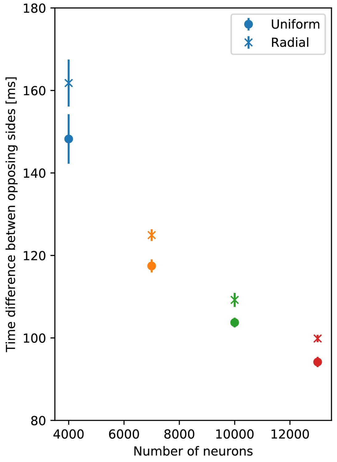
Comparison of propagation speed in DNNs.
Delay between initiation of DNN activity and its reaching of the opposing side, as a function of the number of DNN neurons (similar to Figure 14). Neurite orientation in these nerve nets is either uniform or has a radial bias.
Figure 17

The jellyfish model.
(A) We model the jellyfish subumbrella as a disc with radius 2.25 cm. The MNN somata are embedded in an annulus with an outer radius of 2 cm and an inner radius of 0.5 cm (gray hatched), leaving the margin and the manubrium region void. We assume that the circular swim muscles (thick red) form discrete sections of concentric circles around the manubrium. The centers of these sections are aligned with the positions of the rhopalia. The DNN is distributed over the annulus between manubrium and margin and the margin with width 0.25 cm (blue hatched). For the hydrodynamics simulations, we use a cross-section of the jellyfish as indicated by the dashed line. (B) We model the spatial geometry of MNN neurites as line segments (rods) and assume that the soma is in their center (discs). Two neurons are synaptically connected if their neurites overlap. The transmission delay is a function of the distances between the somata and the intersection of their line segments (Equation (8)).
Figure 18
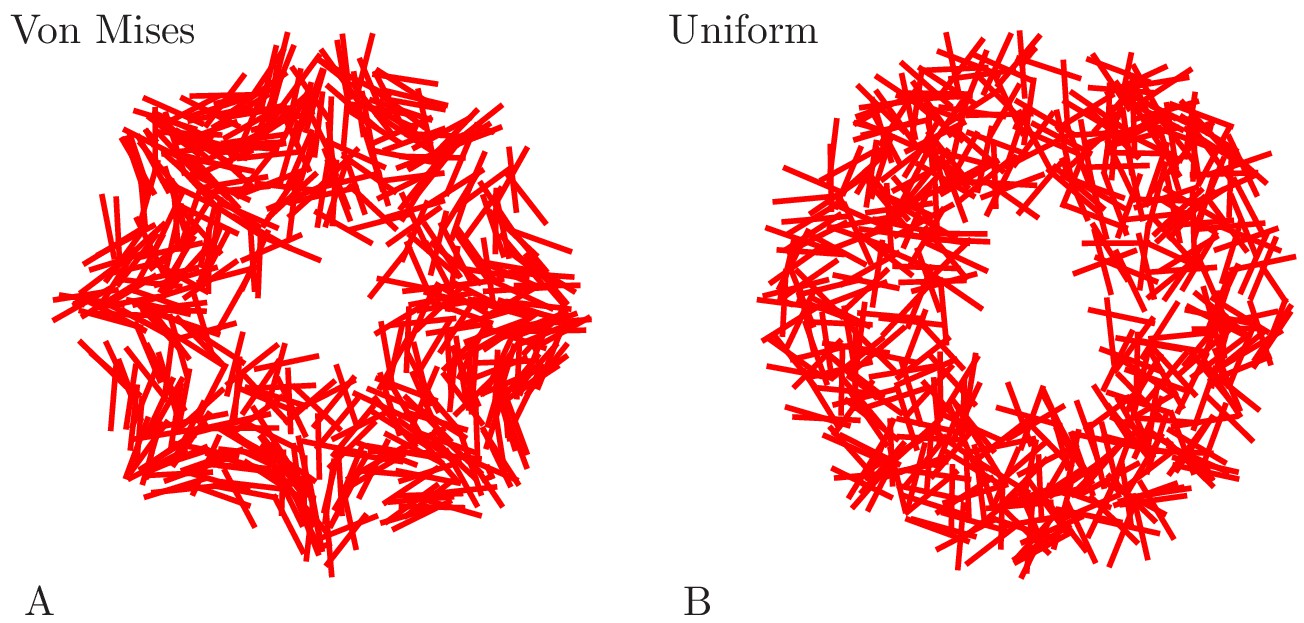
Example MNN models.
Two MNNs consisting of 500 neurons with von Mises (A) or uniformly distributed (B) neurite orientation.
Figure 19

Example DNN model.
(A) A DNN with 3500 Neurons. (B) The DNN (blue) and an MNN with 1000 neurons (red) displayed together. The DNN extends further into the bell margin.
Figure 20
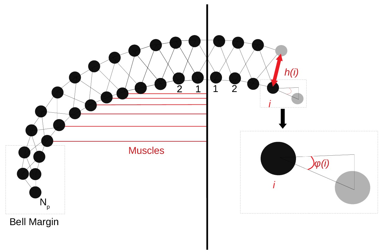
The Jellyfish 2D sectional model.
The 2D structure consists of two rows of vertices, which are connected by damped springs (black lines). The placement of the vertices in the subumbrella (bottom row) depends only on the angle (Equation (14)). The vertices in the exumbrella (top row) are placed at a distance (Equation (15)) perpendicular to the curve traced by the bottom vertices. The circular muscles (red lines), which contract the bell, create a force (Equation (12)) toward the imaginary center line of the jellyfish. No circular muscles are present at the center of the bell and the bell margin.
Tables
Table 1
Neuron model parameters.
| Variable | Value | Unit |
|---|---|---|
| 1 | pF | |
| 345 | nS | |
| 39.8 | nS | |
| 27.2 | nS | |
| 10.8 | nS | |
| 953 | pS | |
| 76.7 | mV | |
| -84.6 | mV | |
| -70 | mV | |
| 1.77 | ||
| 4.82 | ||
| 8.64 | ||
| 2.51 | ||
| 3.85 | ||
| 1.15 | ||
| 1 | ||
| -2.02 | mV | |
| -10.94 | mV | |
| 2.4 | mV | |
| 2.21·10-2 | mV | |
| 10.65 | mV | |
| -10.01 | mV | |
| 48.58 | mV | |
| 3.99 | mV | |
| -13.03 | mV | |
| 22.55 | mV | |
| -8.97 | mV | |
| 26.43 | mV | |
| -4.57 | mV | |
| 22.41 | mV | |
| 5.2·10-1 | ms | |
| 1.3 | ms | |
| 1.65·10-1 | ms | |
| 2.73 | ms | |
| 1.13 | ms | |
| 7.66 | ms | |
| 10.43 | ms | |
| 4.66·10-1 | ms | |
| 2.42·10-1 | ms | |
| 7.51 | ms | |
| 10 | ms | |
| 16.64 | ms | |
| 2 | ms | |
| 4.96 | ms | |
| -5.87·10-1 | mV | |
| 2.68·10-1 | mV | |
| -35.22 | mV | |
| -29.96 | mV | |
| -12.71 | mV | |
| -34 | mV | |
| -39.93 | mV | |
| 1 | mV | |
| 6.62 | mV | |
| 23.12 | mV | |
| 15.13 | mV | |
| 43.6 | mV | |
| 20 | mV | |
| 29.88 | mV |
Table 2
Synapse model parameters.
| Variable | Value | Unit |
|---|---|---|
| 75 | nS | |
| 20 | ms | |
| 3 | ms | |
| 6 | ms | |
| 9.57·10-1 | ||
| 4.32 | mV |
Table 3
Muscle model parameters.
| Variable | Value | Unit |
|---|---|---|
| 1.075 | ||
| 2.15·10-2 | ||
| 0.4 | ||
| for circular muscles | 0.4 | N |
| for radial muscles | 0.8 | N |
Table 4
Fluid Simulation parameters.
| Variable | Value | Unit |
|---|---|---|
| 0.005 | Ns/m2 | |
| 1000 | kg/m2 | |
| Time step | 10-5 | s |
| x-length of Eulerian grid | 0.06 | m |
| y-length of Eulerian grid | 0.08 | m |
| x-grid size | 180 | |
| y-grid size | 240 |
Table 5
Geometry parameters.
| Variable | Value | Unit |
|---|---|---|
| 0.5 | ||
| 224 | ||
| 1 | ||
| 2 | ||
| 0.5 | mm | |
| 6 | mm | |
| 3000 | ||
| 2·107 | N/m | |
| 8·107 | N/m | |
| 2.5 | kg/s |
Additional files
Download links
A two-part list of links to download the article, or parts of the article, in various formats.
Downloads (link to download the article as PDF)
Open citations (links to open the citations from this article in various online reference manager services)
Cite this article (links to download the citations from this article in formats compatible with various reference manager tools)
From single neurons to behavior in the jellyfish Aurelia aurita
eLife 8:e50084.
https://doi.org/10.7554/eLife.50084


