Deep sampling of Hawaiian Caenorhabditis elegans reveals high genetic diversity and admixture with global populations
- Northwestern University, United States
- New York University, United States
Figures
Figure 1 with 2 supplements
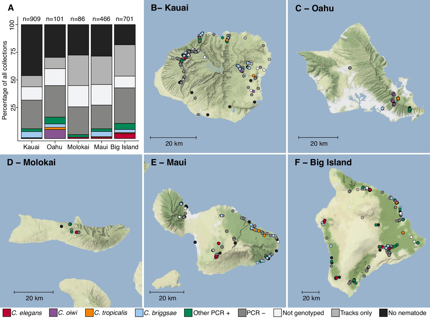
Geographic distribution of sampling sites across five Hawaiian islands.
In total we sampled 2263 unique sites. (A) The percentage of each collection category is shown by island. The collection categories are colored according to the legend at the bottom of the panel, and the total number of samples for each island are shown above the bars. (B–F) The circles indicate unique sampling sites (n = 2,263) and are colored by the collection categories shown in the bottom legend. For sampling sites where multiple collection categories apply (n = 299), the site is colored by the collection category shown in the legend from left to right, respectively. For all sampling sites, the GPS coordinates and collection categories found at that site are included in (Source data 1). We focused our studies on Caenorhabditis nematode collections, excluding C. kamaaina because it was only found at two sampling sites.
© 2019, Thunderforest. Maps in Panels B-F adapted from Thunderforest under a CC BY-NC-SA 2.0 license.
-
Figure 1—source data 1
The collection categories and location data for each of the 2263 samples collected are organized here.
The c_label column indicates the unique ID for each sample collected. The collection_type column indicates which collection class into which the sample was placed. The island column indicates which island from which the sample was collected. The PCR_positive column contains a 0 for samples that had a PCR product with the Rhabditid primers but did not have PCR product with the ITS2 primers. The worms_on_sample column is ‘Yes’ if worms were observed on the collection plate, ‘No’ if they were not observed, or ‘Tracks’ if we only saw tracks on the plate. Longitude and Latitude columns indicate the GPS position of the sample. The multiple_type column is ‘no’ if only one collection_type was observed for the c_label and ‘yes’ if more than one collection type was observed. (Used to generate Figure 1A–F).
- https://cdn.elifesciences.org/articles/50465/elife-50465-fig1-data1-v2.csv
Figure 1—figure supplement 1
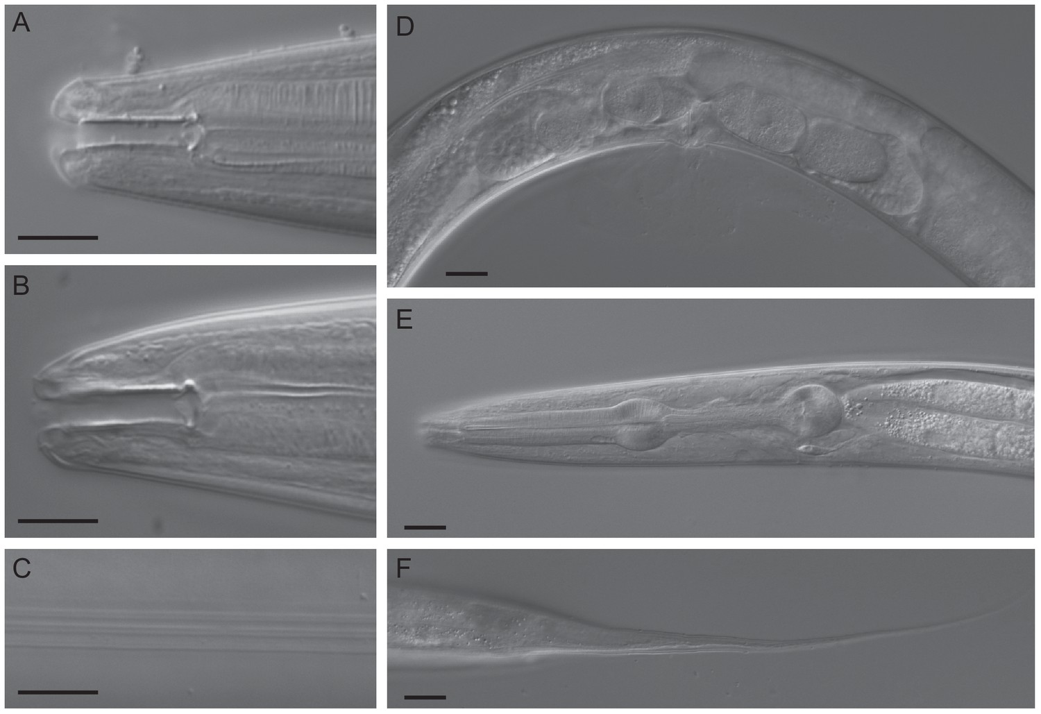
DIC micrographs of C. oiwi sp. n.
(A) stoma of male (subventral right, dorsal is up); (B) stoma of female subventral right, dorsal is up); (C) female lateral field with alae; (D) female midbody region showing vulva, one embryo in each uterus, one oocyte in each spermatheca and part of the posterior ovary (left side view); (E) pharynx region of female (left side view); and (F) female tail (left side view). Scale bars in A-C are 10 µm and 20 µm in D-F. A formal description of C. oiwi is provided (Appendix 1).
Figure 1—figure supplement 2
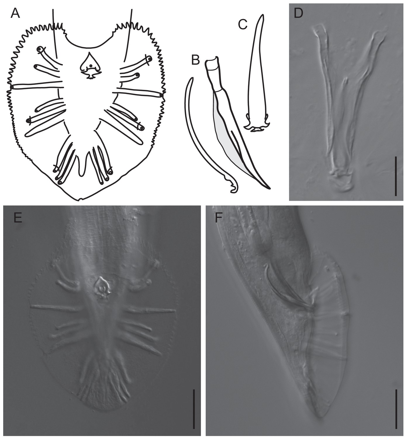
Features of the male tail of C.oiwi sp. n.
(A) Drawing of the male tail in ventral view. The rays in position 1, 5 and 7 (from anterior) open to the dorsal side of the fan. (B) A drawing of the spicule and guernaculum in right lateral view is shown. (C) A drawing of the gubernaculum in ventral view is shown. (D) DIC micrograph of the spicules and gubernaculum in ventral view is shown. (E, F) DIC micrographs of the male tail in ventral (E) and lateral right view (F) are shown. Scale bars are 20 µm. A formal description of C. oiwi is provided (Appendix 1).
Figure 2
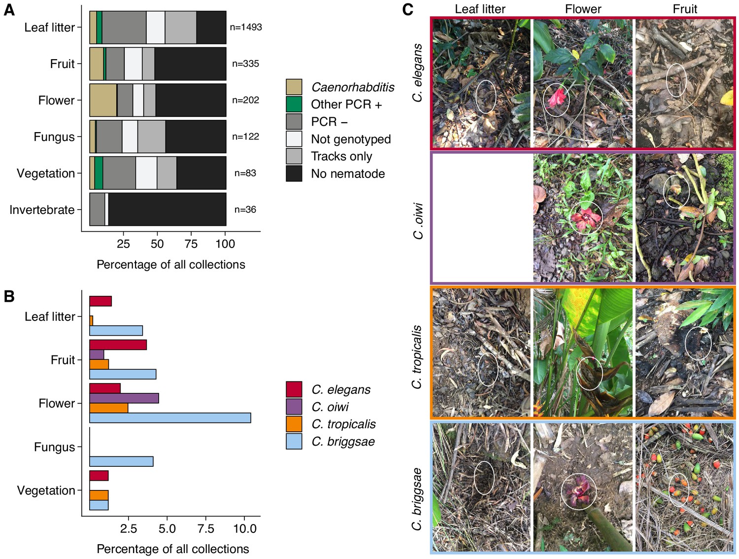
Collection categories by substrate type.
(A) The percentage of each collection category is shown by substrate type. The collection categories are colored according to the legend at the right, and the total number of samples for each substrate are shown to the right of bars. (B) The percentage of collections is shown by substrate type for each Caenorhabditis species (excluding C. kamaaina, n = 2). (C) Examples of substrate photographs for Caenorhabditis species are shown and white ellipses indicate what was sampled. The C. oiwi leaf litter cell is blank because C. oiwi was only isolated from flowers and fruit.
-
Figure 2—source data 1
The fraction of samples in each collection category organized by major substrate classes.
The fixed_substrate column indicates the substrate category. The worm_per_substrate column indicates how many instances of that collection category were sampled within the substrate class. The total_substrates column indicates how many substrates of that class were sampled in total. The perc_worm_sub column indicates the fraction of samples in that belong to a certain collection category within each substrate class. The plot_type column indicates the various collection categories. (These data were used to generate Figure 2A).
- https://cdn.elifesciences.org/articles/50465/elife-50465-fig2-data1-v2.csv
-
Figure 2—source data 2
The fraction of samples containing each Caenorhabditis species by substrate class are organized here.
The invertebrate substrate class is not included because we did not sample Caenorhabditis from that class. The species_family column indicates the Caenorhabditis species under consideration for that row of data. The fixed_substrate column indicates the substrate class. The perc_worm_sub2 column indicates the fraction of samples containing each Caenorhabditis species by substrate class. (These data were used to generate Figure 2B).
- https://cdn.elifesciences.org/articles/50465/elife-50465-fig2-data2-v2.csv
Figure 3 with 3 supplements
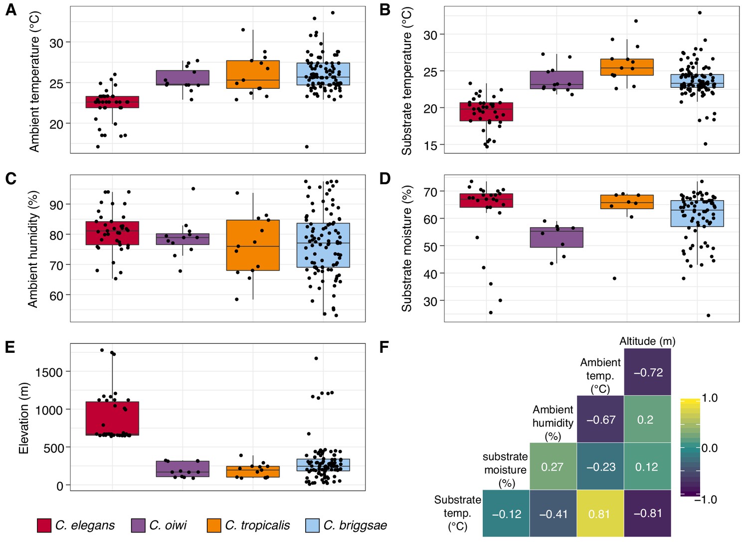
Environmental parameter values for sites where Caenorhabditis species were isolated.
(A–E) Tukey box plots are plotted by species (colors) for different environmental parameters. Each dot corresponds to a unique sampling site where that species was identified. In cases where two Caenorhabditis species were identified from the same sample (n = 3), the same parameter values are plotted for both species. All p-values were calculated using Kruskal-Wallis test and Dunn test for multiple comparisons with p values adjusted using the Bonferroni method; comparisons not mentioned were not significant (α = 0.05). (A) Ambient temperature (°C) was typically cooler at the sites were C. elegans were isolated compared to sites for all other Caenorhabditis species (Dunn test, p<0.005). (B) Substrate temperature (°C) was also generally cooler for C. elegans than all other Caenorhabditis species (Dunn test, p<0.00001). (C) Ambient humidity (%) did not differ significantly among the Caenorhabditis-positive sites. (D) Substrate moisture (%) was generally greater for C. elegans than C. oiwi (Dunn test, p=0.002). (E) Elevation (meters) was typically greater at sites where C. elegans were isolated compared to sites for all other Caenorhabditis species (Dunn test, p<0.00001). (F) A correlation matrix for the environmental parameters was made using sample data from the Caenorhabditis species shown. The parameter labels for the matrix are printed on the diagonal, and the Pearson correlation coefficients are printed in the cells. The color scale also indicates the strength and sign of the correlations shown in the matrix.
-
Figure 3—source data 1
Environmental parameter data for all Caenorhabditis-positive collections are organized here.
The c_label column indicates the unique ID for each sample collected. The s_label column is the unique ID for each nematode isolated. The species_family column corresponds to the species isolated from that isolation plate. The env_par column indicated the environmental parameter being measured in the value column. The KM_pvalue indicates the p-value of the Kruskal-Wallis rank sum test for each environmental parameter. (Used to generate Figure 3A–E).
- https://cdn.elifesciences.org/articles/50465/elife-50465-fig3-data1-v2.csv
-
Figure 3—source data 2
Pearson correlation coefficients for environmental parameter pairs.
The X and Y columns correspond to the environmental parameters tested for correlations. The pearson_correlation column indicates the Pearson correlation coefficients for the parameter pairs. (Used to generate Figure 3F).
- https://cdn.elifesciences.org/articles/50465/elife-50465-fig3-data2-v2.csv
Figure 3—figure supplement 1
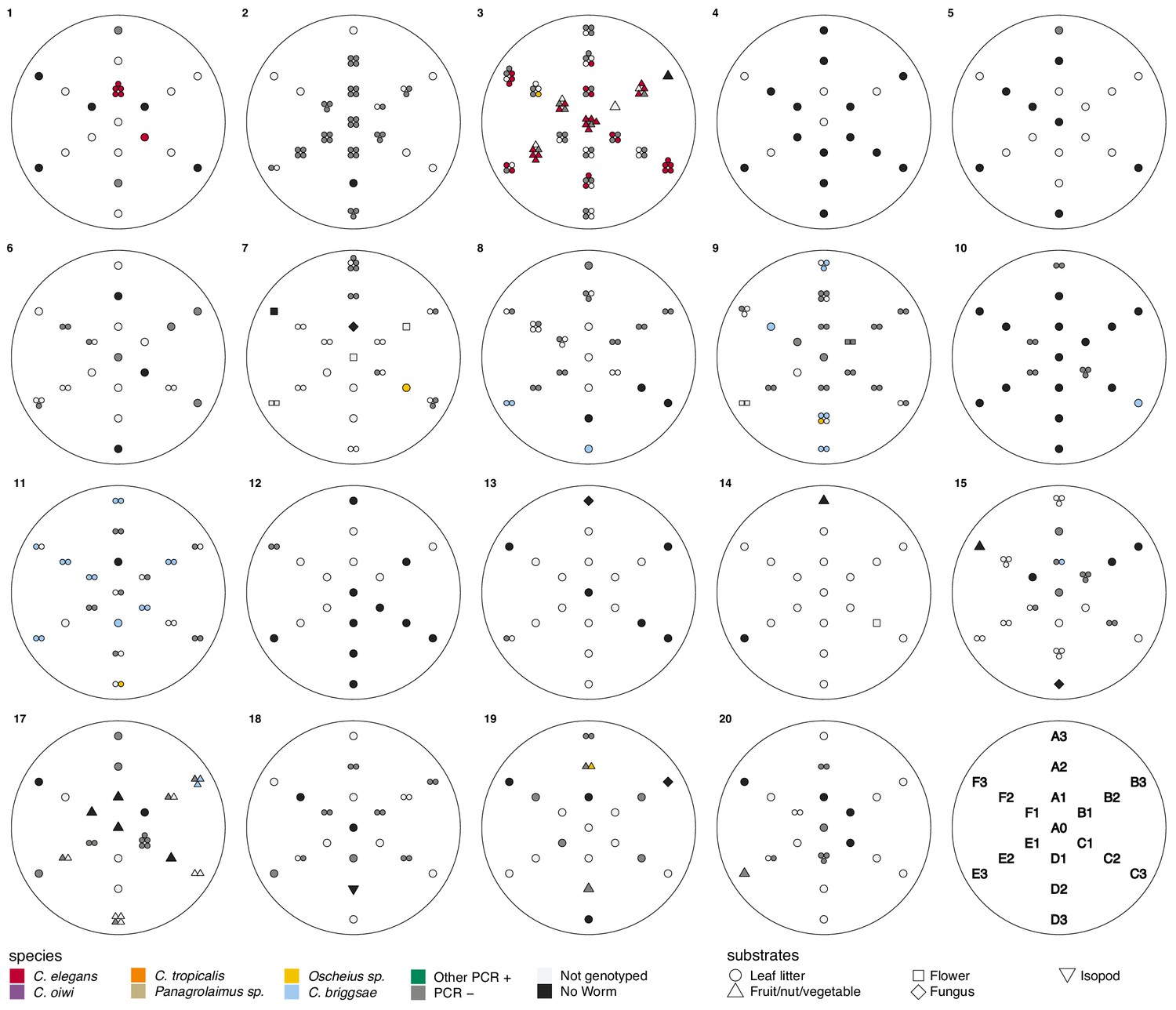
Local scale sampling with gridsects.
Nineteen of twenty gridsects are shown. A key defining the sample positions for each gridsect is shown on the lower right. Samples were collected in six directions (A–F), each 60° apart. The center is denoted as A0, and samples were collected in each direction at one, two, and three meters from the center. Gridsect 16 is omitted because it was incomplete. The colors and shapes plotted at gridsect positions show the collection category and substrate class collected at that position as defined in the plot legend. We isolated multiple nematodes from some substrates, in these cases multiple shapes are plotted at that position to indicate the various collection categories that were found there.
-
Figure 3—figure supplement 1—source data 1
Collection data for all gridsect samples.
(Used to generate Figure 3—figure supplement 1).
- https://cdn.elifesciences.org/articles/50465/elife-50465-fig3-figsupp1-data1-v2.csv
Figure 3—figure supplement 2
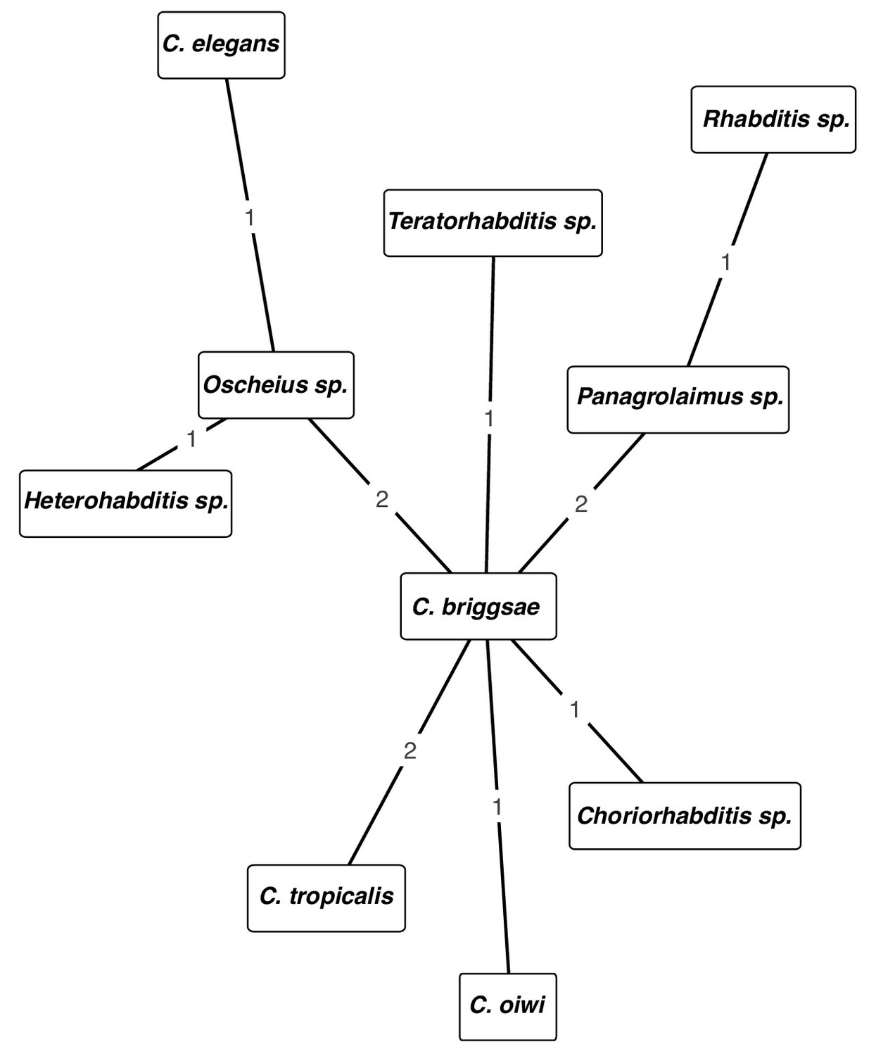
Network of cohabiting species isolated from samples.
The nodes are labeled with the taxa. The edges are labeled with the number of times the taxa shown on the nodes were isolated from the same sample.
-
Figure 3—figure supplement 2—source data 1
Collection data for all samples where two or more PCR-positive nematodes were isolated from the same sample.
(Used to generate Figure 3—figure supplement 2).
- https://cdn.elifesciences.org/articles/50465/elife-50465-fig3-figsupp2-data1-v2.csv
Figure 3—figure supplement 3
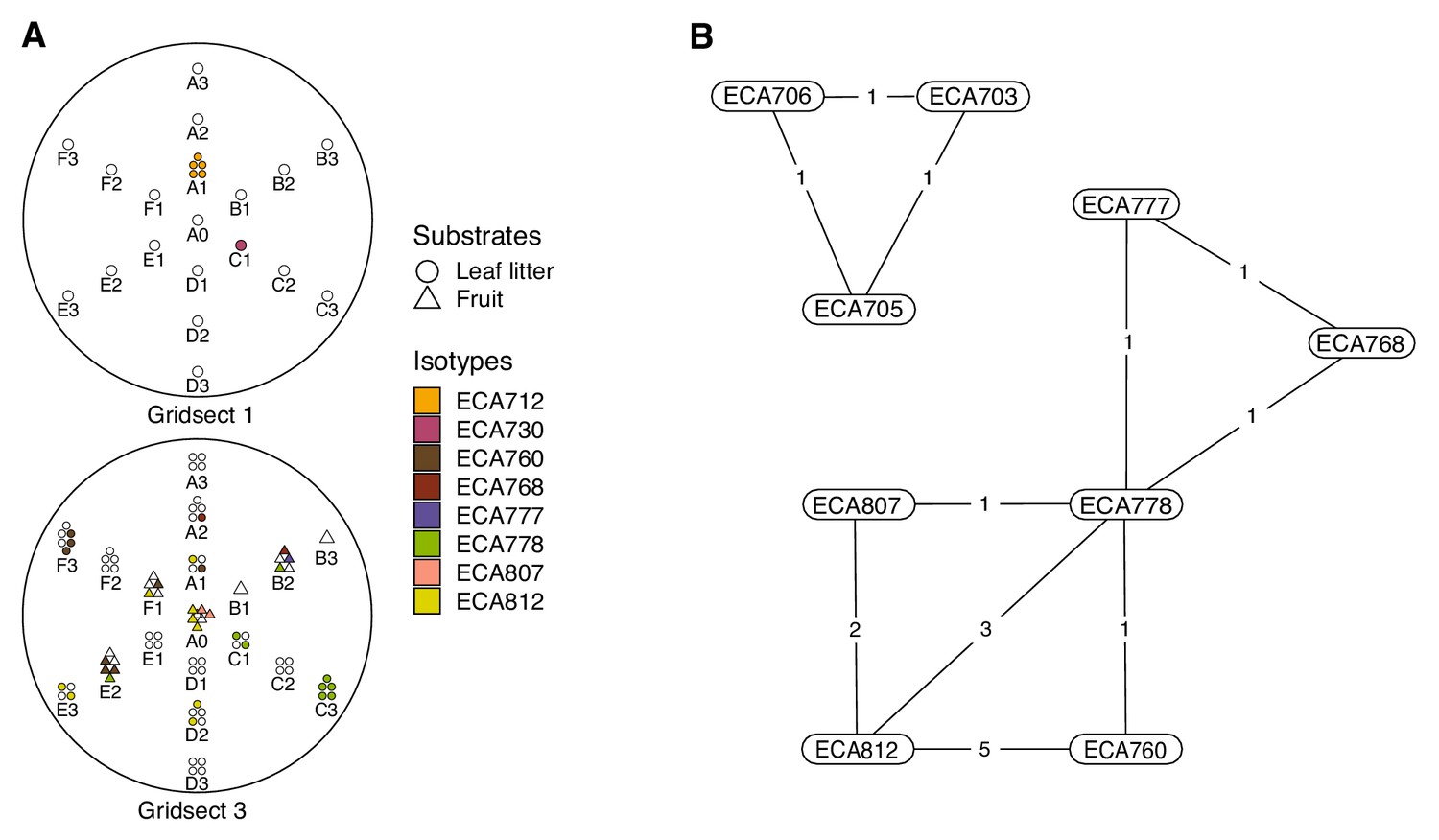
Local diversity and colocalization of isotypes.
(A) Local scale gridsect sampling is shown. Each gridsect contains a total of 19 samples centered on the sample position labeled A0. The remaining sample positions are labeled by one of six transect lines (A–F) followed by the distance (in meters) from position A0. The shapes plotted above the position label show the collection category at that position as defined in the plot legend, and the colors correspond to C. elegans isotypes in the legend. Samples that did not contain C. elegans strains are colored white. (B) A colocalization network is shown for C. elegans isotypes from all Hawaiian samples. The numbers inset on the lines connecting two isotypes correspond to the number of unique samples where the two strains were isolated together.
-
Figure 3—figure supplement 3—source data 1
Collection data for gridsects from which C. elegans were isolated.
(Used to generate Figure 3—figure supplement 3A).
- https://cdn.elifesciences.org/articles/50465/elife-50465-fig3-figsupp3-data1-v2.csv
-
Figure 3—figure supplement 3—source data 2
Collection data for all samples from which multiple C. elegans isotypes were isolated.
(Used to generate Figure 3—figure supplement 3B).
- https://cdn.elifesciences.org/articles/50465/elife-50465-fig3-figsupp3-data2-v2.csv
Figure 4 with 1 supplement
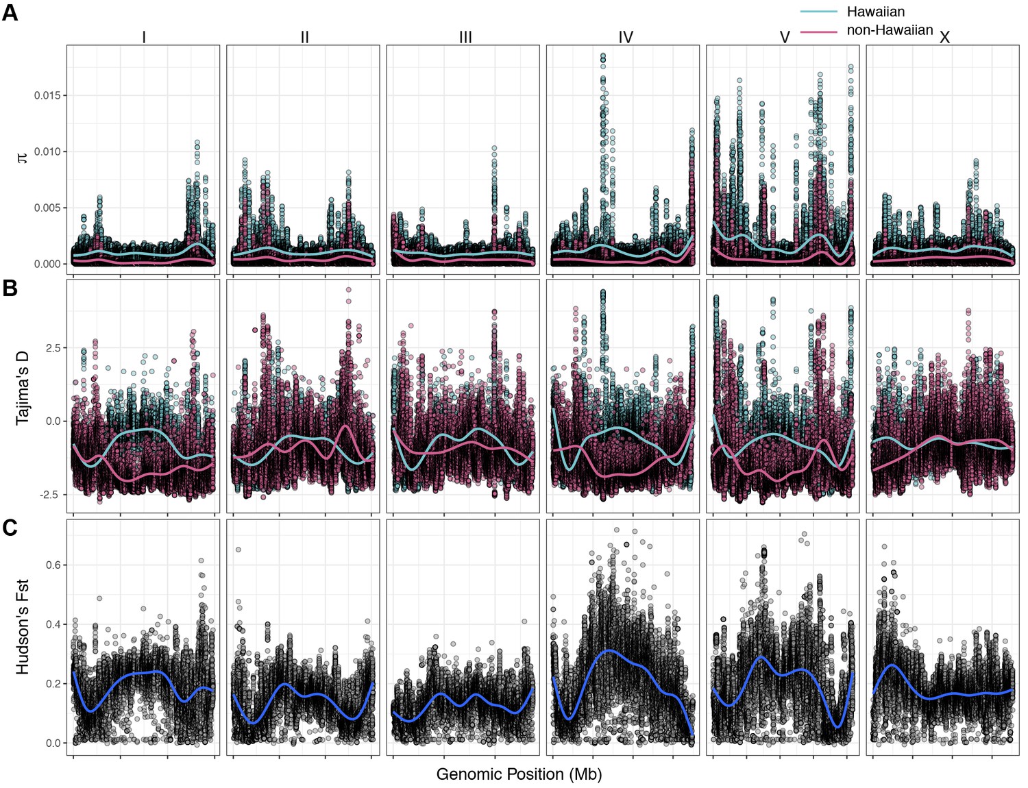
Chromosomal patterns of C. elegans diversity and differentiation.
All comparisons are between the 43 Hawaiian isotypes and the 233 non-Hawaiian isotypes from the rest of the world. All statistics were calculated along a sliding window of size 10 kb with a step size of 1 kb. Each dot corresponds to the calculated value for a particular window. (A) Genome-wide π calculated for Hawaiian isotypes (light blue) and non-Hawaiian isotypes (pink) are shown. (B) Genome-wide Tajima’s D statistics for Hawaiian isotypes (light blue) and non-Hawaiian isotypes (pink) are shown. (C) Genome-wide Hudson’s FST comparing the Hawaiian and non-Hawaiian isotypes are shown.
-
Figure 4—source data 1
Chromosomal patterns of C. elegans diversity and differentiation.
The values of nucleotide diversity (𝜋) for 10 kb windows in the Hawaiian and non-Hawaiian samples are found in the Diversity_Hawaiian and Diversity_non-Hawaiian columns, respectively. The snp_index, position, and CHROM columns indicate the index ID, nucleotide position, and chromosome start points for each of the 10 kb windows. The Fst column holds Hudson’s FST values indicating differentiation among the two samples for the same windows. (Used to generate Figure 4A and C).
- https://cdn.elifesciences.org/articles/50465/elife-50465-fig4-data1-v2.csv
-
Figure 4—source data 2
Chromosomal patterns of Tajima’s D for the Hawaiian and non-Hawaiian samples.
The CHROM and position columns indicate the chromosome and nucleotide starting positions for the 10 kb windows used to calculate Tajima’s D. The Population column corresponds to the sample being tested, and the value column indicates the value of the Tajima’s D statistic calculated for each window. (Used to generate Figure 4B).
- https://cdn.elifesciences.org/articles/50465/elife-50465-fig4-data2-v2.csv
Figure 4—figure supplement 1
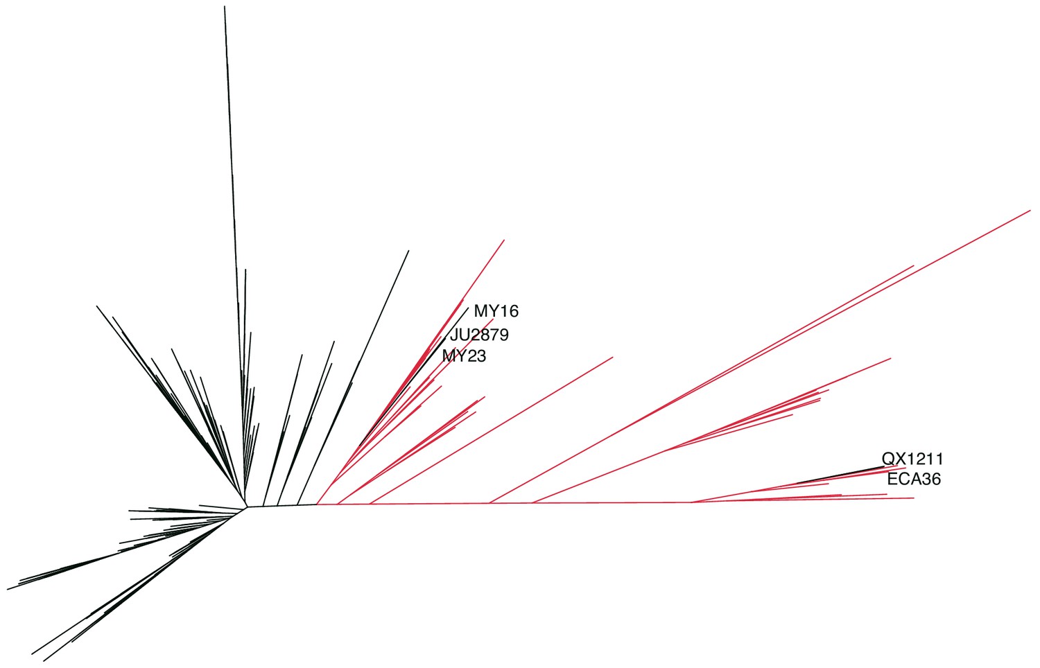
Caenorhabditis elegans unrooted tree for 276 isotypes.
A maximum likelihood tree built using single nucleotide variants found in the 276 C. elegans isotypes sampled, including the 26 new Hawaiian isotypes. (Substitution model: GTR+FO). The isotypes labeled in red were isolated from the Hawaiian Islands (n = 43). The five isotypes labeled are non-Hawaiian isotypes that group within the Hawaiian isotypes.
-
Figure 4—figure supplement 1—source data 1
Best-scoring maximum likelihood tree output from RAxML-ng.
(Used to generate Figure 4—figure supplement 1).
- https://cdn.elifesciences.org/articles/50465/elife-50465-fig4-figsupp1-data1-v2.zip
Figure 5 with 4 supplements
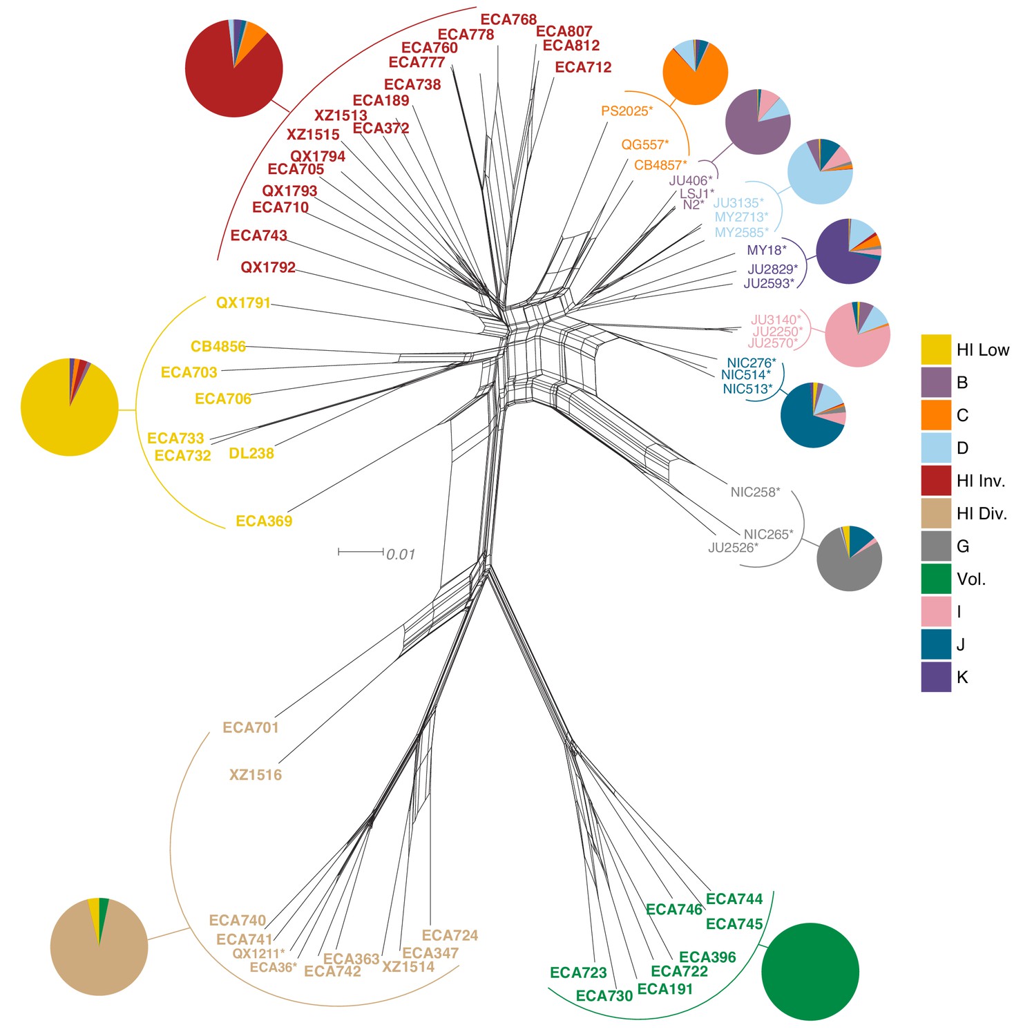
Relatedness of the Hawaiian C. elegans isotypes.
Neighbor-joining net showing the genetic relatedness of the Hawaiian C. elegans isotypes relative to a representative set of non-admixed, non-Hawaiian isotypes from each population defined by ADMIXTURE (K = 11). Colors of isotype names indicate the maximum fraction of population assignment from ADMIXTURE (K = 11), including the seven non-Hawaiian populations (B–K) and the four Hawaiian populations (Hawaiian Invaded, Hawaiian Low, Hawaiian Divergent, and Volcano). Isotypes labeled with an asterisk are representative of non-admixed, non-Hawaiian isotypes from each population defined by ADMIXTURE (K = 11). Pie charts represent population proportions for all isotypes within the full admixture population.
-
Figure 5—source data 1
VCF used to generate the nexus file with vcf2phylip.py script for the neighbor-joining network shown in Figure 5.
This VCF is processed from the ‘PopGen VCF’ (Supplementary data 3 on GitHub https://github.com/AndersenLab/HawaiiMS/blob/master/data/elife_files/Supplemental_Data_3.vcf.gz; see Materials and methods - Phylogenetic analyses). (Used to generate Figure 5).
- https://cdn.elifesciences.org/articles/50465/elife-50465-fig5-data1-v2.zip
-
Figure 5—source data 2
The nexus file for creating neighbor-joining network shown in Figure 5.
This file was generated from the VCF (Figure 5—source data 1) using the vcf2phylip.py script (see Materials and methods - Phylogenetic analyses). (Used to generate Figure 5).
- https://cdn.elifesciences.org/articles/50465/elife-50465-fig5-data2-v2.zip
-
Figure 5—source data 3
Admixture population proportions for all isotypes within each admixture population (K = 11).
The pop-assignment column indicates the admixture population. The n column is the number of isotypes assigned to that admixture population. The cluster column corresponds to each of the 11 admixture populations identified labelled as perc_a – perc_k. The cluster_perc column indicates the fraction of each cluster found within all n isotypes assigned to each admixture population. The total_perc column indicates the sum of all cluster_perc values for each admixture population. (Used to generate pie charts in Figure 5).
- https://cdn.elifesciences.org/articles/50465/elife-50465-fig5-data3-v2.csv
Figure 5—figure supplement 1
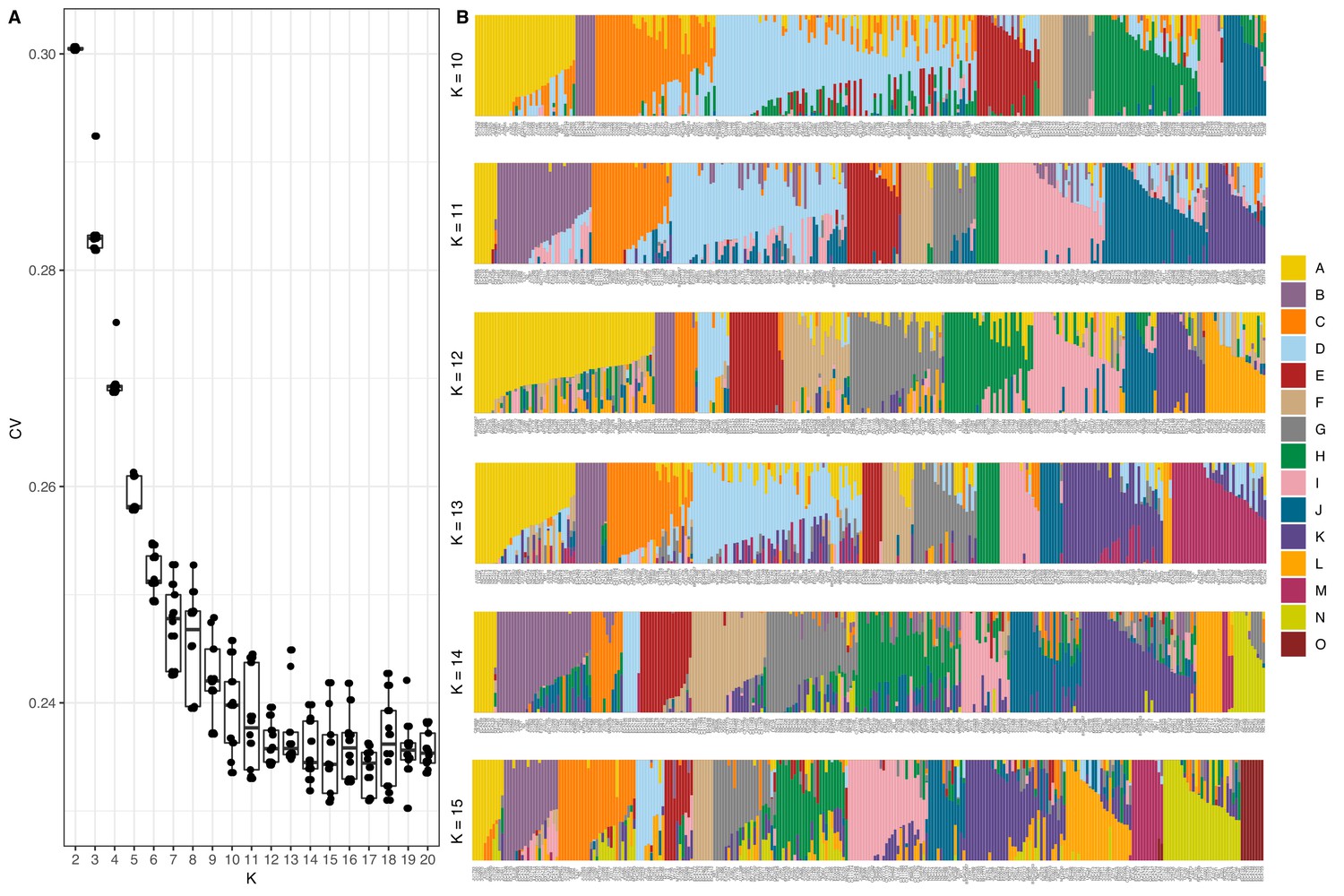
Summary of ADMIXTURE analysis.
(A) Tukey boxplots of ten independent ADMIXTURE runs showing the cross-validation error on the y-axis for the number of populations (K) ranging from 2 to 20 on the x-axis. (B) The inferred population proportions estimated by ADMIXTURE are shown on the y-axis of the all C. elegans isotypes on the x-axis. Each isotype is represented by a vertical line, which is partitioned into colored segments that represent the isotype’s membership fractions for the populations shown in the legend.
-
Figure 5—figure supplement 1—source data 1
Cross-validation error from ten Independent ADMIXTURE runs at Ks 2–20.
(Used to generate Figure 5—figure supplement 1A).
- https://cdn.elifesciences.org/articles/50465/elife-50465-fig5-figsupp1-data1-v2.csv
-
Figure 5—figure supplement 1—source data 2
The inferred population proportions estimated by ADMIXTURE for all isotypes at Ks 10–15.
(Used to generate Figure 5—figure supplement 1B).
- https://cdn.elifesciences.org/articles/50465/elife-50465-fig5-figsupp1-data2-v2.csv
Figure 5—figure supplement 2
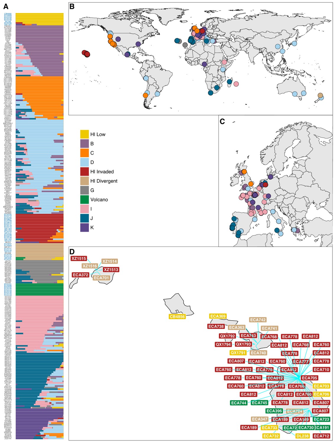
Global population structure.
(A) The inferred population proportions estimated by ADMIXTURE (K = 11) with C. elegans isotype names on the y-axis. The names colored in blue represent Hawaiian isotypes. (B) The global distribution of all 276 isotypes are shown with colors corresponding to the legend. Colors are assigned based on the largest ancestral population fraction for that isotype (e.g. the isotype MY23 from Germany was assigned as 51% ‘Hawaii Invaded’ and 49% global ‘K’ but it is colored red on the map for ‘Hawaii Invaded’). (C) The same data are shown but with more resolution in Europe. (D) All distinct collections of Hawaiian isotypes are shown with labels for isotype names colored by the ancestral population assignment. The blue lines point to specific collection locations for those isotypes. The cluster of ‘Hawaiian Invaded’ isotypes on the Big Island correspond to gridsect three and adjacent collections from the Kalōpā state recreation area.
-
Figure 5—figure supplement 2—source data 1
The sampling locations and admixture population assignment for all strains including isotype reference strains.
(Used to generate Figure 5—figure supplement 2B–D).
- https://cdn.elifesciences.org/articles/50465/elife-50465-fig5-figsupp2-data1-v2.csv
-
Figure 5—figure supplement 2—source data 2
The inferred population proportions estimated by ADMIXTURE for all isotypes at K = 11.
(Used to generate Figure 5—figure supplement 2A).
- https://cdn.elifesciences.org/articles/50465/elife-50465-fig5-figsupp2-data2-v2.csv
Figure 5—figure supplement 3
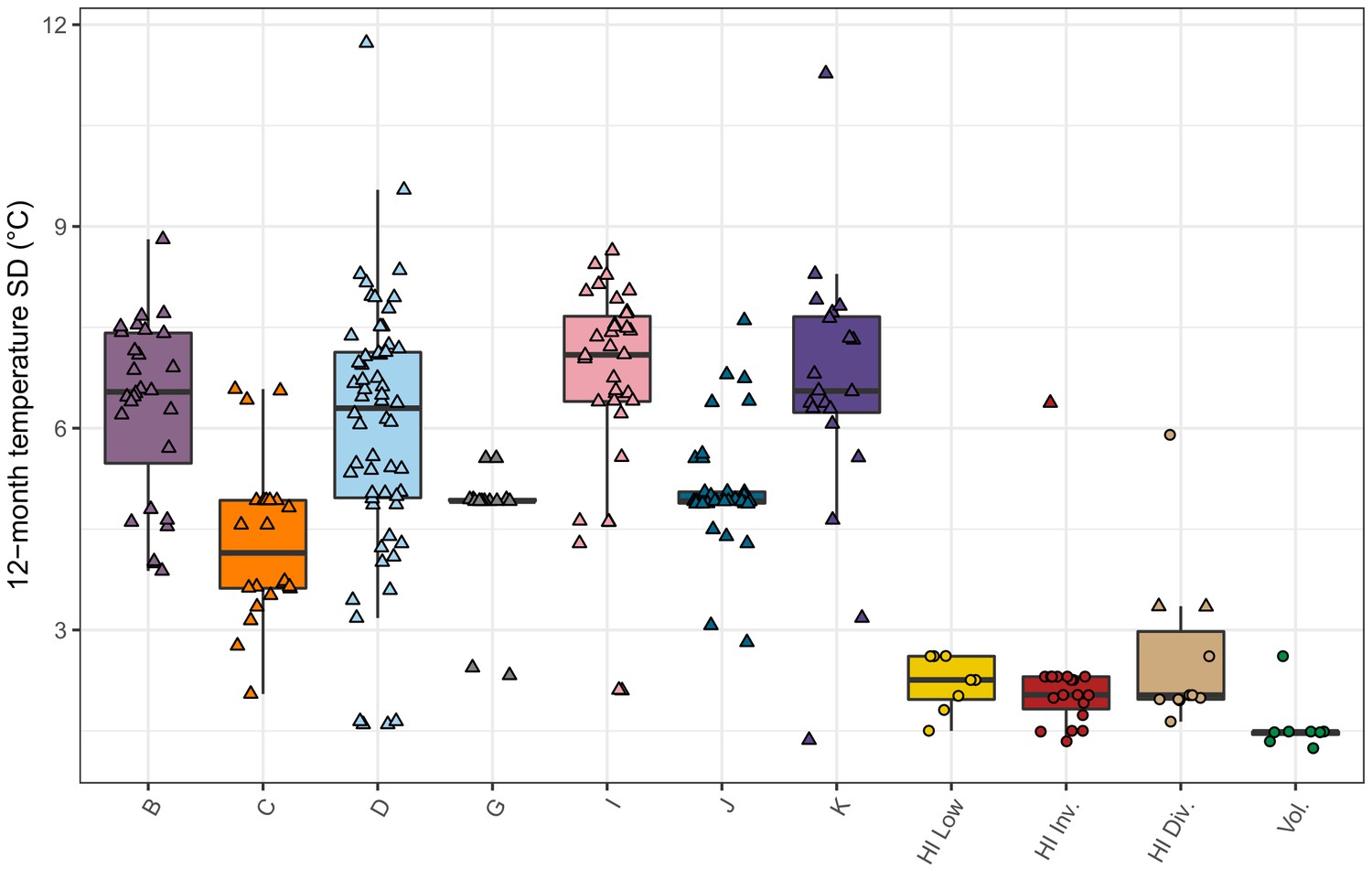
Seasonal temperature variation by population.
The standard deviation of daily mean temperatures for a 12-month period centered on the collection date for each isolate is shown. If only the year of collection is known, then the 12-month period is centered on January 1 st of that year, and if the year and month are known but not the exact date, then the 12-month period is centered on the first of that month. The data points correspond to isotypes and are colored by their assigned populations from admixture analysis. The Hawaiian isotypes are plotted as circles and non-Hawaiian isotypes are plotted as triangles.
-
Figure 5—figure supplement 3—source data 1
Seasonal temperature variation for all isotypes over a 12-month period.
The data are taken from weather stations nearest to the isolation locations. (Used to generate Figure 5—figure supplement 3).
- https://cdn.elifesciences.org/articles/50465/elife-50465-fig5-figsupp3-data1-v2.csv
Figure 5—figure supplement 4
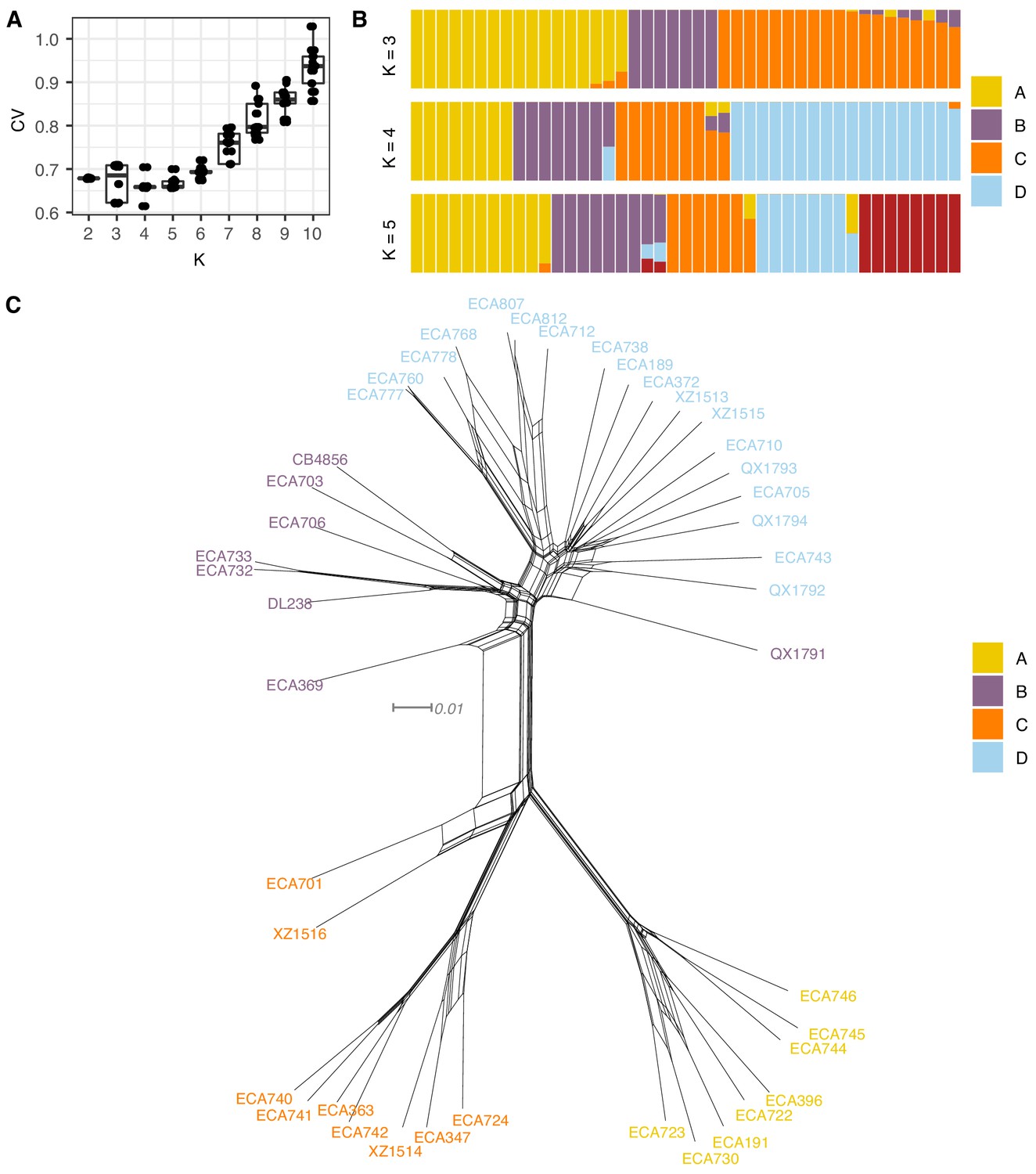
Summary of ADMIXTURE analysis on Hawaiian C. elegans isotypes.
(A) Tukey boxplots of ten independent ADMIXTURE runs showing the cross-validation error on the y-axis for the population number (K) ranging from 2 to 10 on the x-axis. (B) The inferred population proportions estimated by ADMIXTURE are shown on the y-axis for the Hawaiian C. elegans isotypes on the x-axis. Each isotype is represented by a vertical line, which is partitioned into colored segments that represent the isotype’s membership fractions in the clusters shown in the legend. (C) A neighbor-joining net showing the genetic relatedness of the Hawaiian isotypes is shown. Colors of labels indicate the largest fractional population assignment from ADMIXTURE (K = 4).
-
Figure 5—figure supplement 4—source data 1
The inferred population proportions estimated by ADMIXTURE for all Hawaiian isotypes at Ks 3–5.
(Used to generate Figure 5—figure supplement 4B).
- https://cdn.elifesciences.org/articles/50465/elife-50465-fig5-figsupp4-data1-v2.csv
-
Figure 5—figure supplement 4—source data 2
Cross-validation error from ten Independent ADMIXTURE runs with only the Hawiian isotypes across Ks 2–10.
(Used to generate Figure 5—figure supplement 4A).
- https://cdn.elifesciences.org/articles/50465/elife-50465-fig5-figsupp4-data2-v2.csv
-
Figure 5—figure supplement 4—source data 3
The nexus file for creating the neighbor-joining network.
(Used to generate Figure 5—figure supplement 4C).
- https://cdn.elifesciences.org/articles/50465/elife-50465-fig5-figsupp4-data3-v2.zip
Figure 6 with 2 supplements
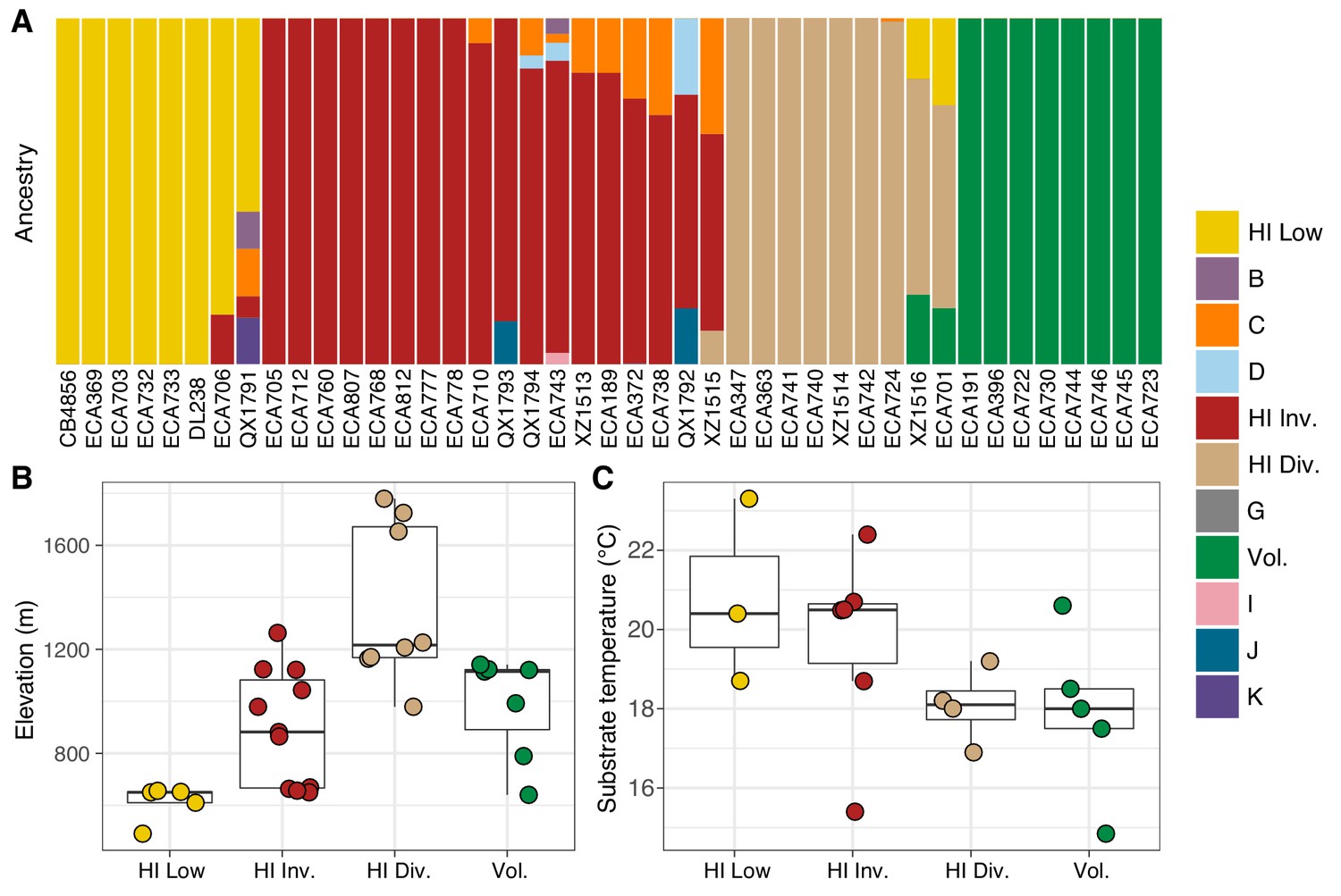
Environmental parameters of Hawaiian C. elegans populations.
(A) The inferred ancestral population fractions for each Hawaiian isotype as estimated by ADMIXTURE (K = 11; 276 C. elegans isotypes) are shown. The bar colors represent the fraction of population assignments from ADMIXTURE for the isotypes named on the x-axis. (B–C) Tukey box plots are shown by population assignments (colors) for different environmental parameters. We used the average values of environmental parameters from geographically clustered collections to avoid biasing our results by local oversampling (See Materials and methods - Environmental parameter analysis). All p-values were calculated using Kruskal-Wallis test and Dunn test for multiple comparisons with p values adjusted using the Bonferroni method; comparisons not mentioned were not significant (α = 0.05). (B) The collection site elevations for Hawaiian isotypes colored by population assignments are shown. The Hawaiian Low and the Hawaiian Invaded populations were typically found at lower elevations than the Hawaiian Divergent population (Dunn test, p-values=0.000168, and 0.037 respectively). (C) The substrate temperatures for Hawaiian isotypes colored by population assignments are shown.
-
Figure 6—source data 1
The inferred population fractions for each Hawaiian isotype as estimated by ADMIXTURE (K = 11; 276 C. elegans isotypes).
The isotype column gives the isotype name. The max_pop_frac colum indicates the largest population fraction for any of the 11 populations estimated by ADMIXTURE for that isotype. The pop_assignment column contains the admixture population (A – K) with the largest population fraction for that isotype. The Hawaiian column is ‘TRUE’ if the isotype was isolated in Hawaii. The cluster column indicates the admixture population under consideration for that isotype. The frac_cluster column is the fraction of each admixture population estimated for each isotype. (Used to generate Figure 6A).
- https://cdn.elifesciences.org/articles/50465/elife-50465-fig6-data1-v2.csv
-
Figure 6—source data 2
Environmental parameters for distinct collections of admixture populations in Hawaii.
In cases where multiple collections were made within 20 meters for the same admixture population, we took the average parameter values for plotting and statistical calculations (see Materials and methods – Environmental parameter analysis). (Used to generate Figure 6B–C).
- https://cdn.elifesciences.org/articles/50465/elife-50465-fig6-data2-v2.csv
-
Figure 6—source data 3
post hoc Dunn multiple comparison tests for differences in environmental parameters among the Hawaiian populations identified by ADMIXTURE are organized here.
(Used to generate Figure 6B–C).
- https://cdn.elifesciences.org/articles/50465/elife-50465-fig6-data3-v2.csv
Figure 6—figure supplement 1
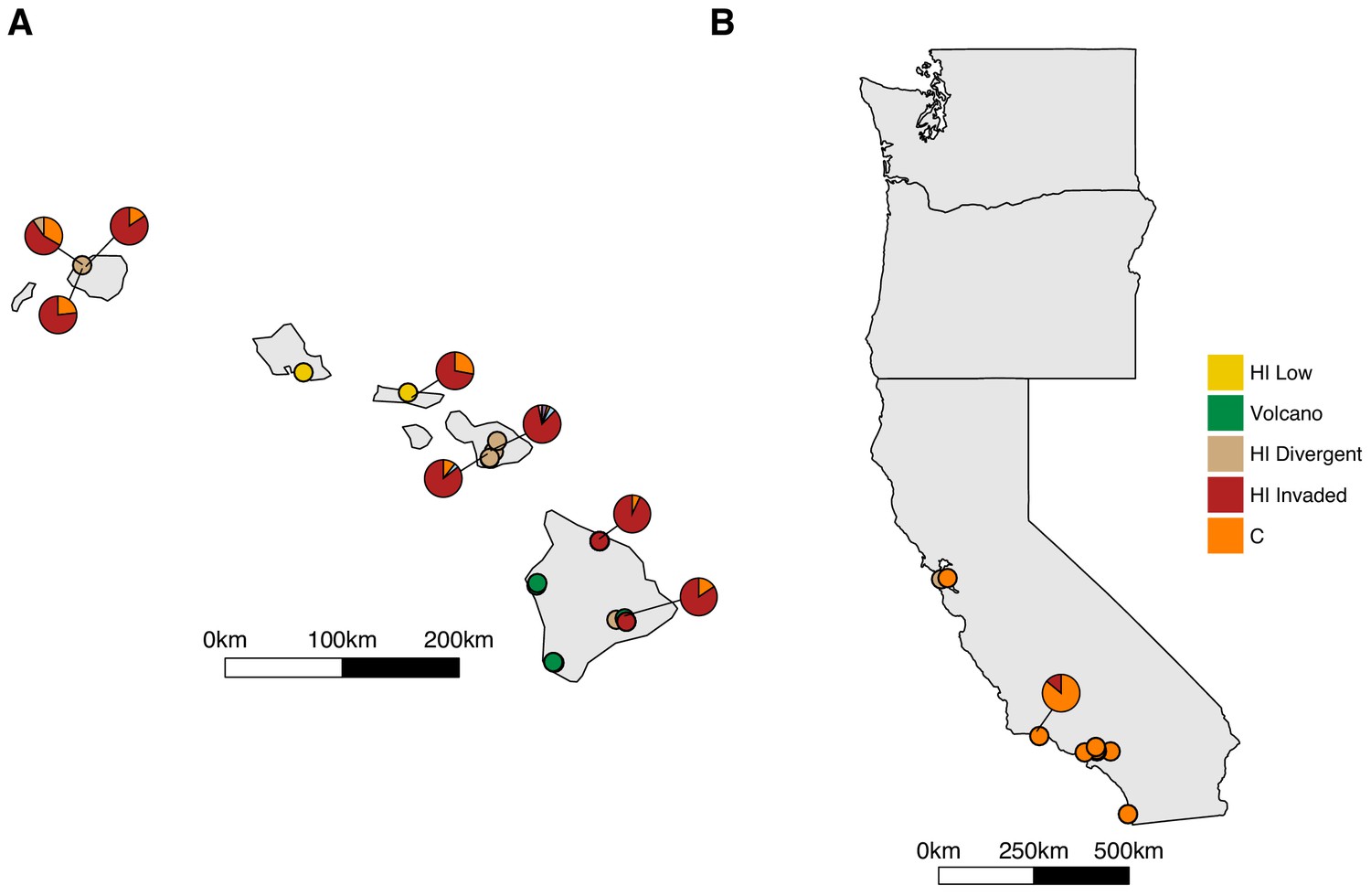
Admixture between the Hawaii Invaded and the global C populations.
Unique isolation locations for non-admixed isotypes from the four Hawaiian populations and the global C population (solid circles) are shown for Hawaii (A) and the west coast of the United States (B). Unique isolation locations for isotypes from the Hawaiian Invaded and global C populations that are admixed with one another (pie charts) are shown for Hawaii (A) and the west coast of the United States (B). The colors correspond to the admixture populations in the legend.
-
Figure 6—figure supplement 1—source data 1
Isolation location data for distinct isolations of all isotypes and their inferred population proportions estimated by ADMIXTURE.
(Used to generate Figure 6—figure supplement 1).
- https://cdn.elifesciences.org/articles/50465/elife-50465-fig6-figsupp1-data1-v2.csv
Figure 6—figure supplement 2

Admixture between the ‘Hawaiian Invaded and ‘global C’ populations.
The fraction of admixture among the three populations is shown on a ternary plot. The data points correspond to isotypes and are colored by the highest fractional population assignment.
-
Figure 6—figure supplement 2—source data 1
The inferred population proportions estimated by ADMIXTURE (K = 11) for isotypes assigned to the Hawaii Invaded, Volcano, and non-Hawaiian C populations.
(Used to generate Figure 6—figure supplement 2).
- https://cdn.elifesciences.org/articles/50465/elife-50465-fig6-figsupp2-data1-v2.csv
Figure 7 with 2 supplements
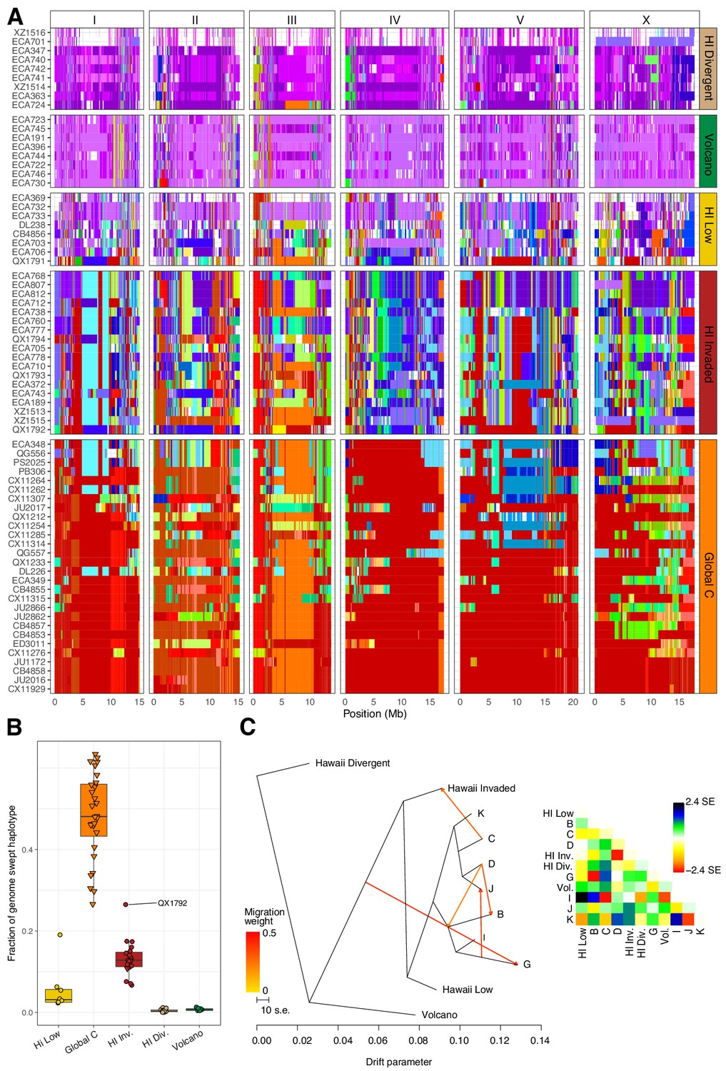
Evidence of migration between the Hawaiian and world populations.
(A) The haplotypes or inferred blocks of identity by descent (IBD) across the genome are shown. The genomic position is plotted on the x-axis for each isotype plotted on the y-axis. The block colors correspond to a uniquely defined IBD group. The dark red blocks correspond to the most common global haplotype (i.e., the swept haplotypes on chr I, IV, V, and left of X). Genomic regions with no color represent regions for which no IBD groups could be determined. The four Hawaiian populations are shown in the top four facets, excluding non-Hawaiian isotypes. The bottom facet shows the non-Hawaiian C population. (B) The total fraction of the genome with the swept haplotype is shown by population. The data points correspond to isotypes and are colored by their assigned populations. The Hawaiian isotypes are plotted as circles and non-Hawaiian isotypes are plotted as triangles. Hawaiian isotypes with greater than 25% of their genome swept are labelled. (C) The inferred relationship among the populations allowing for five migration events (ADMIXTURE, K = 11). The heat map to the right represents the residual fit to the migration model.
-
Figure 7—source data 1
Haplotypes or IBD blocks across the genomes of all 276 isotypes are organized here.
(Used to generate Figure 7A).
- https://cdn.elifesciences.org/articles/50465/elife-50465-fig7-data1-v2.csv
-
Figure 7—source data 2
Fraction of the genome with the swept haplotypes for each isotype in the four Hawaiian populations and the non-Hawaiian C population.
(Used to generate Figure 7B).
- https://cdn.elifesciences.org/articles/50465/elife-50465-fig7-data2-v2.csv
-
Figure 7—source data 3
Ancestry fractions (.Q file) and allele frequencies of the inferred ancestral populations (.P file) from ADMIXTURE analysis.
(These data are used to generate Figure 7C).
- https://cdn.elifesciences.org/articles/50465/elife-50465-fig7-data3-v2.zip
Figure 7—figure supplement 1
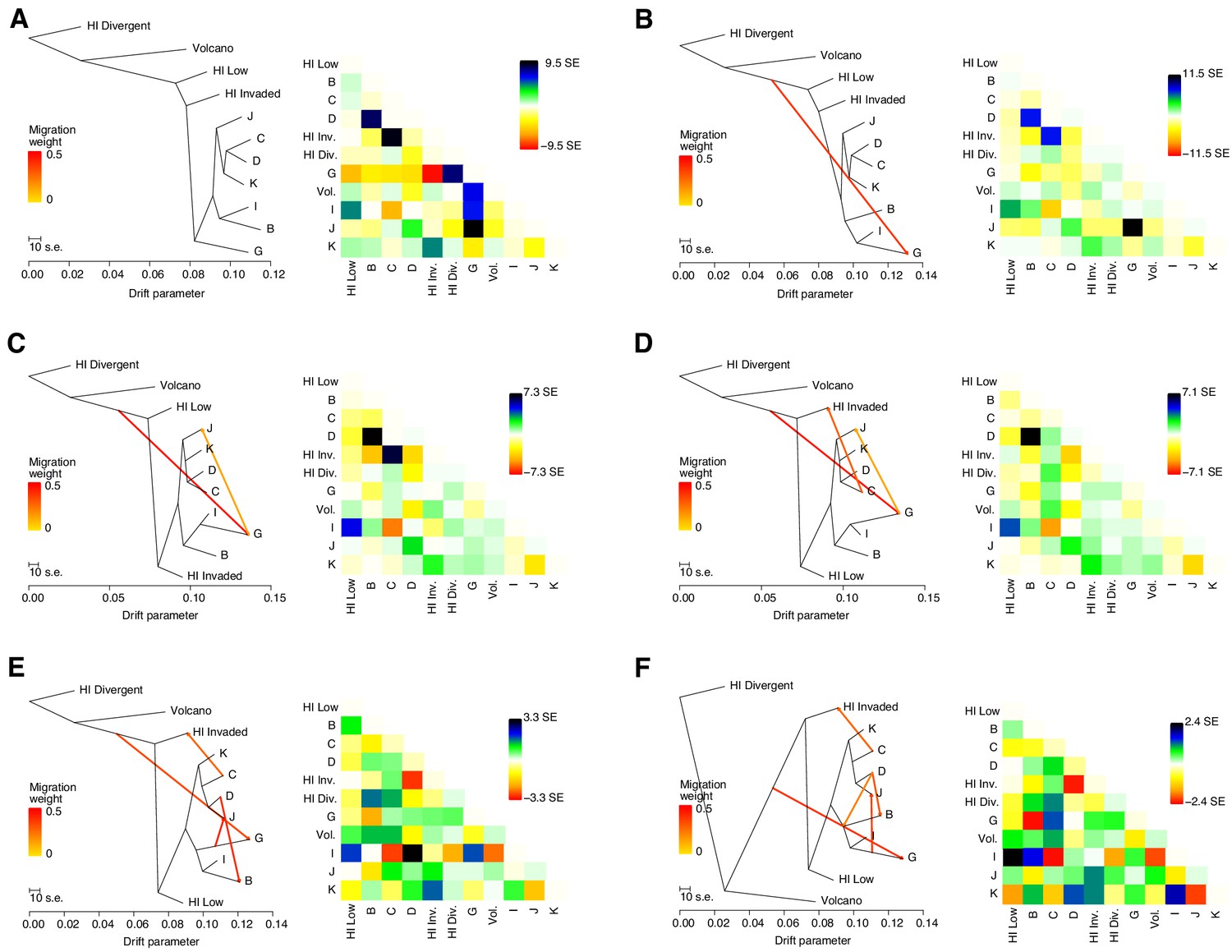
Evidence of migration between Hawaiian and non-Hawaiian populations.
(A–D) The inferred relationships among the populations (ADMIXTURE, K = 11) with zero (A), one (B), two (C), three (D), four (E), or five (F) migration events. The right panels contain heat maps corresponding to the residual fit to the migration models.
-
Figure 7—figure supplement 1—source data 1
Ancestry fractions (.Q file) and allele frequencies of the inferred ancestral populations (.P file) from ADMIXTURE analysis (K = 11).
(Used to generate Figure 7—figure supplement 1A–F).
- https://cdn.elifesciences.org/articles/50465/elife-50465-fig7-figsupp1-data1-v2.zip
Figure 7—figure supplement 2
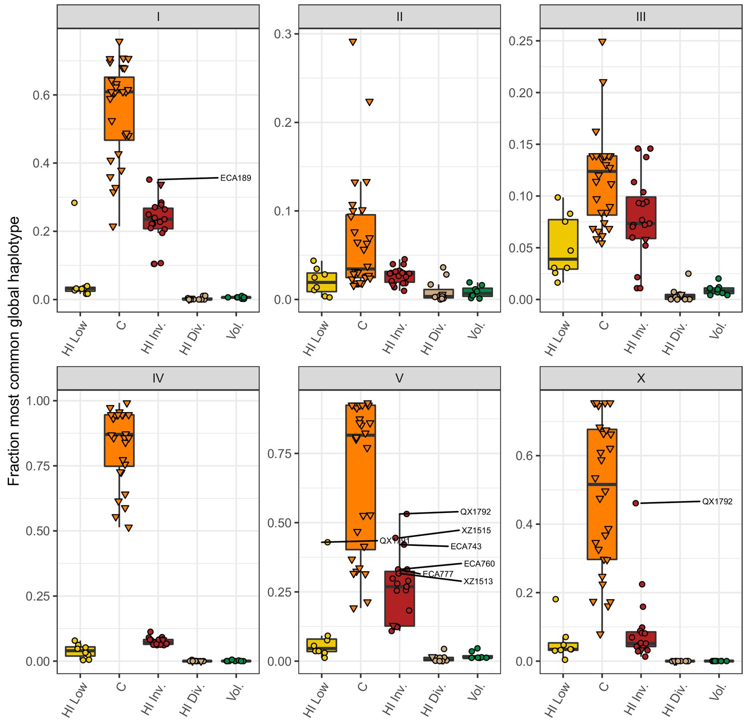
Most common global haplotype sharing by chromosome and population.
The fraction of each chromosome that belongs to the most common global haplotype is shown on the y-axis. The data points correspond to isotypes and are colored by their assigned populations. The Hawaiian isotypes are plotted as circles and non-Hawaiian isotypes are plotted as triangles. Hawaiian isotypes with greater than 30% of a chromosome belonging to the most common global haplotype are labelled in the chromosome facet. The most common global haplotype is synonymous with the globally swept haplotype on chromosomes I, IV, V, and the left of X.
-
Figure 7—figure supplement 2—source data 1
Fraction of each chromosome with the most common global haplotype (swept haplotypes for chromosomes I, IV, V, and X) for each isotype in the four Hawaiian populations and the non-Hawaiian C population.
Source data 1: Complete sampling data for the collections and isolations completed for this study as a. csv file. Source data 2: Cryopreserved strains that are available upon request, including any known alternative names that might be used in the literature. Supplementary Data 3: Variants among the 276 isotypes referred to as the ‘PopGen VCF’.
- https://cdn.elifesciences.org/articles/50465/elife-50465-fig7-figsupp2-data1-v2.csv
Tables
Key resources table
| Reagent type (species) or resource | Designation | Source or reference | Identifiers | Additional information |
|---|---|---|---|---|
| Sequence-based reagent | oECA305; ITS2 F primer | This paper | Andersen Lab: oECA305 F primer | GCTGCGTTATTTACCACGAATTGCARAC |
| Sequence-based reagent | oECA202; ITS2 R primer | 10.1186/1471-2148-11-339 | Andersen Lab: oECA202 R primer | GCGGTATTTGCTACTACCAYYAMGATCTGC |
| Sequence-based reagent | RHAB1350F; Rhabditid F primer | 10.1093/molbev/msh264 | Andersen Lab: oECA1271 | TACAATGGAAGGCAGCAGGC |
| Sequence-based reagent | RHAB1868R; Rhabditid R primer | 10.1093/molbev/msh264 | Andersen Lab: oECA1272 | CCTCTGACTTTCGTTCTTGATTAA |
| Commercial assay or kit | Blood and Tissue DNA isolation kit | QIAGEN | cat# 69506 | |
| Commercial assay or kit | Qubit dsDNA Broad Range Assay Kit | Invitrogen | cat# Q32850 | |
| Software, algorithm | Fulcrum | Spatial Networks | Spatial Networks: Fulcrum | https://www.fulcrumapp.com/ |
| Software, algorithm | UGENE | 10.1093/bioinformatics/bts091 | Unipro: UGENE v.1.27.0 | http://ugene.net/ |
| Software, algorithm | Nextflow | 10.1038/nbt.3820 | Nexflow | https://github.com/nextflow-io/nextflow |
Additional files
-
Source data 1
Complete sampling data for the collections and isolations completed for this study as a .csv file.
- https://cdn.elifesciences.org/articles/50465/elife-50465-data1-v2.csv
-
Source data 2
Cryopreserved strains that are available upon request, including any known alternative names that might be used in the literature.
- https://cdn.elifesciences.org/articles/50465/elife-50465-data2-v2.csv
-
Supplementary file 1
Collection categories identified on each island.
Multiple collection categories were found for some samples. For this reason, the total number of distinct collections (2,594) exceeds the total number of samples (2,263).
- https://cdn.elifesciences.org/articles/50465/elife-50465-supp1-v2.docx
-
Supplementary file 2
Description of variant sets used in this study.
The additional filters applied to the PopGen VCF for specific uses are described in methods.
- https://cdn.elifesciences.org/articles/50465/elife-50465-supp2-v2.docx
-
Supplementary file 3
Nematode field sampling data form.
- https://cdn.elifesciences.org/articles/50465/elife-50465-supp3-v2.docx
-
Supplementary file 4
Nematode isolation data form.
- https://cdn.elifesciences.org/articles/50465/elife-50465-supp4-v2.docx
-
Supplementary file 5
Nextflow pip elines used in our study.
- https://cdn.elifesciences.org/articles/50465/elife-50465-supp5-v2.docx
-
Transparent reporting form
- https://cdn.elifesciences.org/articles/50465/elife-50465-transrepform-v2.pdf
Download links
A two-part list of links to download the article, or parts of the article, in various formats.
Downloads (link to download the article as PDF)
Open citations (links to open the citations from this article in various online reference manager services)
Cite this article (links to download the citations from this article in formats compatible with various reference manager tools)
Deep sampling of Hawaiian Caenorhabditis elegans reveals high genetic diversity and admixture with global populations
eLife 8:e50465.
https://doi.org/10.7554/eLife.50465


