Male meiotic spindle features that efficiently segregate paired and lagging chromosomes
- Experimental Center, Faculty of Medicine Carl Gustav Carus, Technische Universität Dresden, Germany
- Zuse Institute Berlin, Germany
- Light Microscopy Imaging Center, Indiana University, United States
- Department of Biology, San Francisco State University, United States
- Max Planck Institute of Molecular Cell Biology and Genetics, Germany
- Max Planck Institute for the Physics of Complex Systems, Germany
- Centre for Systems Biology Dresden, Germany
Figures
Figure 1 with 1 supplement

Unpaired chromosomes lag in spermatocyte meiosis I.
(A) Time series of confocal image projections of meiosis I (M I) and meiosis II (M II) in males with microtubules (β-tubulin::GFP, green) and chromosomes (histone H2B::mCherry, red). Anaphase onset is time point zero (t = 0). White arrowheads mark the unpaired X chromosome position. Right panels show corresponding kymographs with chromosomes in white, microtubules in green. Anaphase onset is marked with a dashed orange line. Scale bars (white), 2 µm; time bar (blue), 2 min. (B) Confocal image projections of spermatocyte meiosis I in wild-type XO males, wild-type XX hermaphrodites, tra-2(e1094) XX males, him-8(e1489) XX hermaphrodites, zim-2(tm574) XX hermaphrodites, zim-2(tm574) XO males and triploid XXO males with centrosomes in green (γ-tubulin::GFP) and chromosomes in red (histone H2B::mCherry). The genotype, sex, number of autosome or X chromosome pairs, and number of unpaired chromosomes is indicated. Still images illustrate the progression of the first meiotic division over time with lagging chromosomes indicated by white arrowheads. In the corresponding kymographs (right panels), chromosomes are shown in white, spindle poles in green. Anaphase onset is marked with a dashed line (orange). Scale bars (white), 2 µm; time bar (blue), 2 min.
Figure 1—video 1
Live-cell imaging of meiosis I and II in wild-type males.
This video shows the first and second meiotic division in spermatocytes in living males. The strain was labeled with β-tubulin::GFP (green) and histone H2B::mCherry (red) to visualize microtubules and chromosomes, respectively. Time is given relative to the onset of anaphase I. Scale bar, 2 µm. This video corresponds to Figure 1A.
Figure 2 with 2 supplements
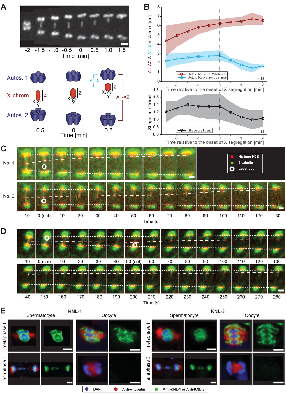
Microtubules associated with the X chromosome exert a pulling force.
(A) Maximum intensity projection images of chromosomes labeled with histone H2B::mCherry (upper panel, white). Time is relative to the onset of segregation of the X chromosome (t = 0). Scale bar, 2 µm. Schematic diagram illustrating the quantification of X chromosome shape (lower panel). The length (Z) of the X chromosome (red) is divided by its width (X + Y divided by two). Autosomes are in blue. (B) Plots showing segregation distances and the shape of the X chromosome in anaphase I spindles (n = 15). The upper panel shows the autosome 1-to-autosome 2 (A1-A2, red) and the autosome 1-to-X chromosome distances (A1-X, blue) over time, the lower panel shows the shape coefficient (black). Solid lines show the mean, shaded areas indicate the standard deviation. The onset of X chromosome movement is given as time point zero (t = 0). (C) Laser microsurgery of microtubules associated with the X chromosome in anaphase I. Microtubules are labeled with β-tubulin::GFP (green) and chromosomes with histone H2B::mCherry (red). The position of the cut is indicated (white circle). Time is relative to the time point of the applied laser cut (t = 0). The position of the autosomes (outer dashed lines) and the X chromosome (inner dashed line) is indicated. The two panels show examples of X chromosome segregation to the applied cut. Scale bars, 2 µm. (D) Example of a double cut experiment over ~300 s. The two cuts are indicated (white circles). Scale bar, 2 µm. (E) Localization of kinetochore proteins in spermatocyte and oocyte meiosis I. Metaphase (upper row in each panel) and anaphase (lower row in each panel) of the first division is shown. Left panels show whole spindles from fixed males stained with antibodies against the kinetochore proteins KNL-1 or KNL-3 (green), microtubules (red), and DAPI (blue). Right panels show the localization patterns of the kinetochore protein only. Scale bars, 2 µm.
-
Figure 2—source data 1
Segregation distances and the shape of the X chromosome in replicates of anaphase I spindles analyzed in Figure 2B .
- https://cdn.elifesciences.org/articles/50988/elife-50988-fig2-data1-v4.xlsx
Figure 2—video 1
Laser ablation of the microtubule bridge in a spermatocyte undergoing the first meiotic division.
Live imaging of anaphase I was performed using an immobilized wild-type male worm labeled with β-tubulin::GFP (green) and histone H2B::mCherry (red) to visualize microtubules and chromosomes, respectively. The applied single laser cut is indicated by a circle. Time is given relative to the laser cut. Scale bar, 2 µm. This video corresponds to Figure 2C (experiment no. 1).
Figure 2—video 2
Double-cut laser ablation of the microtubule bridge in a spermatocyte undergoing first meiotic division.
Live imaging of anaphase I was performed using an immobilized wild-type male worm labeled with β-tubulin::GFP (green) and histone H2B::mCherry (red) to visualize microtubules and chromosomes, respectively. The laser cuts are indicated by circles. Time is given relative to the first laser cut. Scale bar, 2 µm. This video corresponds to Figure 2D.
Figure 3 with 3 supplements
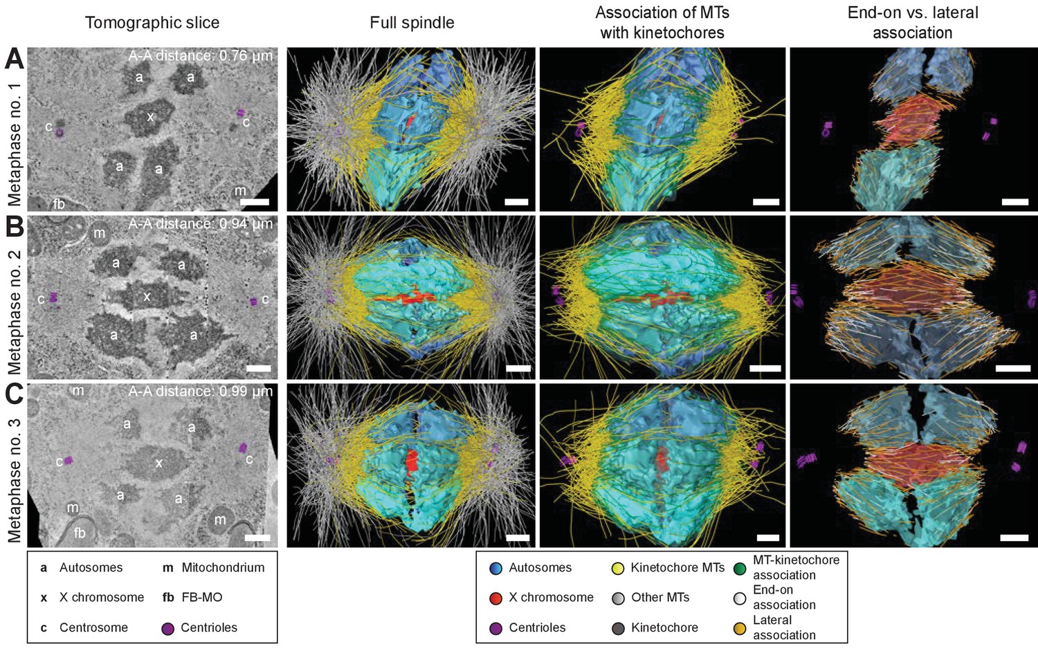
Three-dimensional ultrastructure of spindles in metaphase I.
(A) Early metaphase spindle (Metaphase no. 1) with unstretched chromosomes. (B–C) Metaphase spindles (Metaphase no. 2 and 3) with stretched chromosomes. Left panels: tomographic slices showing the centrosomes (c, with centrioles in purple), the autosomes (a), and the unpaired X chromosome (x) aligned along the spindle axis, mitochondria (m) and fibrous body-membranous organelles (fb). Mid left panels: corresponding three-dimensional models of the full spindles. Autosomes are in different shades of either blue or cyan, the X chromosome in red, centriolar microtubules in purple, microtubules within 150 nm to the chromosome surfaces in yellow, and all other microtubules in gray. Mid right panels: association of kinetochore microtubules with the kinetochores. Kinetochores are shown as semi-transparent regions around each chromosome. The part of each microtubule entering the kinetochore region around the holocentric chromosomes is shown in green. Right panels: visualization of end-on (white) versus lateral (orange) associations of microtubules with chromosomes. Only the parts of microtubules inside of the kinetochore region are shown. The autosome-to-autosome distance (A-A) for each reconstruction is indicated in the left column. Scale bars, 500 nm.
Figure 3—video 1
Full tomographic reconstruction of the metaphase I spindle in a wild-type male spermatocyte.
This video shows a three-dimensional model of the spindle apparatus at metaphase I. Autosomes are shown in different grades of either blue or cyan, the X chromosome in red, centriolar microtubules in purple. Microtubules located within a distance of 150 nm or closer to the chromosome surfaces and displayed in yellow are considered as kinetochore microtubules. All other microtubules are shown in gray. This video corresponds to Figure 3A (Metaphase data set no. 1).
Figure 3—video 2
Full tomographic reconstruction of the metaphase I spindle in a wild-type male spermatocyte.
This video shows stitched serial tomograms through the entire 3D volume of a metaphase I spindle and the corresponding three-dimensional model of the spindle apparatus. Autosomes are shown in different grades of either blue or cyan, the X chromosome in red, centriolar microtubules in purple, kinetochore microtubules in yellow, all other microtubules in gray. This video corresponds to Figure 3B (Metaphase data set no. 2).
Figure 3—video 3
Full tomographic reconstruction of the metaphase I spindle in a wild-type male spermatocyte.
This video shows the three-dimensional model of the spindle apparatus at metaphase I. Autosomes are shown in different grades of either blue or cyan, the X chromosome in red, centriolar microtubules in purple, kinetochore microtubules in yellow, all other microtubules in gray. This video corresponds to Figure 3C (Metaphase data set no. 3).
Figure 4 with 5 supplements

Three-dimensional ultrastructure of spindles in anaphase I.
(A) Spindle at Anaphase onset. (B) Spindle at mid anaphase (Anaphase no. 1) with a pole-to-pole distance of 2.98 µm. (C) Mid anaphase spindle (Anaphase no. 3) with a pole-to-pole distance of 3.35 µm. (D) Mid anaphase spindle (Anaphase no. 4) with a pole-to-pole distance of 3.37 µm. (E) Spindle at late anaphase (Anaphase no. 7) with a pole-to-pole distance of 5.44 µm and the X chromosome with initial segregation to one of the daughter cells. Left panels: tomographic slices showing the centrosomes (c, with centrioles in purple), the autosomes (a), and the unpaired X chromosome (x) aligned along the spindle axis, mitochondria (m) and fibrous body-membranous organelles (fb). Mid left panels: corresponding three-dimensional models illustrating the organization of the full spindle. Autosomes are in different shades of either blue or cyan, the X chromosome in red, centriolar microtubules in purple, microtubules within 150 nm to the chromosome surfaces in yellow, and all other microtubules in gray. Mid right panels: association of kinetochore microtubules with the kinetochores. Kinetochores are shown as semi-transparent regions around each chromosome. The part of each microtubule entering the kinetochore region around the holocentric chromosomes is shown in green. Right panels: visualization of end-on (white) versus lateral (orange) associations of microtubules with chromosomes. Only the parts of microtubules inside of the kinetochore region are shown. The autosome-to-autosome distance (A-A) for each reconstruction is indicated in the left column. Scale bars, 500 nm.
Figure 4—video 1
Full tomographic reconstruction of the spindle in a wild-type male spermatocyte at the onset of anaphase I.
This video shows the three-dimensional model of the spindle apparatus at onset of anaphase I. Autosomes are shown in different grades of either blue or cyan, the X chromosome in red, centriolar microtubules in purple, kinetochore microtubules in yellow, all other microtubules in gray. This video corresponds to Figure 4A.
Figure 4—video 2
Full tomographic reconstruction of the anaphase I spindle in a wild-type male spermatocyte.
This video shows a three-dimensional model of the spindle apparatus in anaphase I. Autosomes are shown in different grades of either blue or cyan, the X chromosome in red, centriolar microtubules in purple, kinetochore microtubules in yellow, all other microtubules in gray. This video corresponds to Figure 4B (Anaphase data set no. 1).
Figure 4—video 3
Full tomographic reconstruction of the anaphase I spindle in a wild-type male spermatocyte.
This video shows a three-dimensional model of the spindle apparatus in anaphase I. Autosomes are shown in different grades of either blue or cyan, the X chromosome in red, centriolar microtubules in purple, kinetochore microtubules in yellow, all other microtubules in gray. This video corresponds to Figure 4C (Anaphase data set no. 3).
Figure 4—video 4
Full tomographic reconstruction of the anaphase I spindle in a wild-type male spermatocyte.
This video shows stitched serial tomograms through the entire 3D volume of the spindle and the corresponding three-dimensional model of the spindle apparatus at anaphase I. Autosomes are shown in different grades of either blue or cyan, the X chromosome in red, centriolar microtubules in purple, kinetochore microtubules in yellow, all other microtubules in gray. This video corresponds to Figure 4D (Anaphase data set no. 4).
Figure 4—video 5
Full tomographic reconstruction of the anaphase I spindle in a wild-type male spermatocyte.
This video shows a three-dimensional model of the spindle apparatus in anaphase I. Autosomes are shown in different grades of either blue or cyan, the X chromosome in red, centriolar microtubules in purple, kinetochore microtubules in yellow, all other microtubules in gray. This video corresponds to Figure 4E (Anaphase data set no. 7).
Figure 5
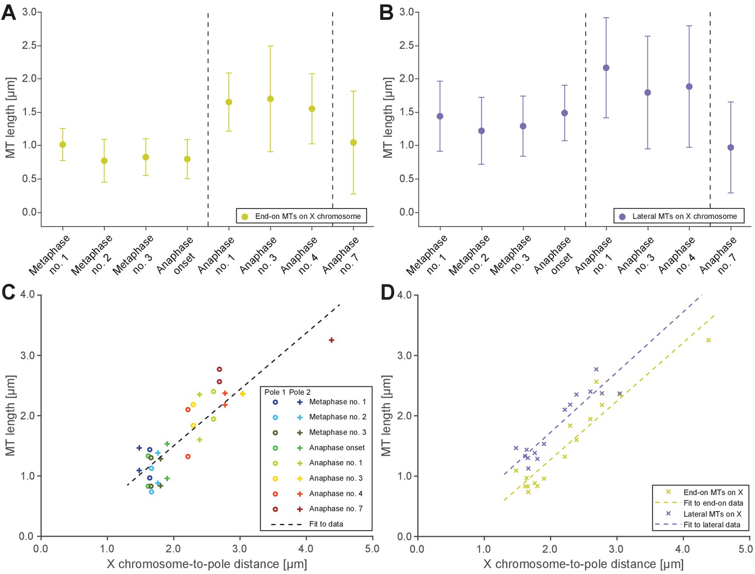
Microtubules that connect the X chromosome to centrosomes are continuous and lengthen during anaphase I.
(A) Length distribution of end-on X chromosome-associated microtubules at different stages of meiosis I. Dots show the mean, error bars indicate the standard deviation. Dashed lines indicate a grouping of the spindles according to the meiotic stages: metaphase/anaphase onset, mid anaphase and late anaphase (see also Appendix 1—figure 2). (B) Length distribution of lateral X chromosome-associated microtubules at different stages of meiosis I. (C) Mean length of microtubules plotted for each side of the X chromosome against the respective X chromosome-to-pole distance (each tomographic data set color-coded). The values for end-on and laterally associated microtubules are given separately. The measurements were performed on all data sets as shown in Figures 3 and 4. A trend line was fitted to indicate the linear relationship between microtubule length and chromosome-to-pole distance. (D) Similar plot as in (C) but end-on (yellow) and laterally (purple) X chromosome-associated microtubules are shown. Two trend lines were fitted to the data sets to illustrate linear relationships independent of the type of association of the microtubules with the X chromosome.
-
Figure 5—source data 1
Measurements of microtubule lengths in spindles shown in Figures 3 and 4 used to generate data in Figure 5.
- https://cdn.elifesciences.org/articles/50988/elife-50988-fig5-data1-v4.xlsx
Figure 6
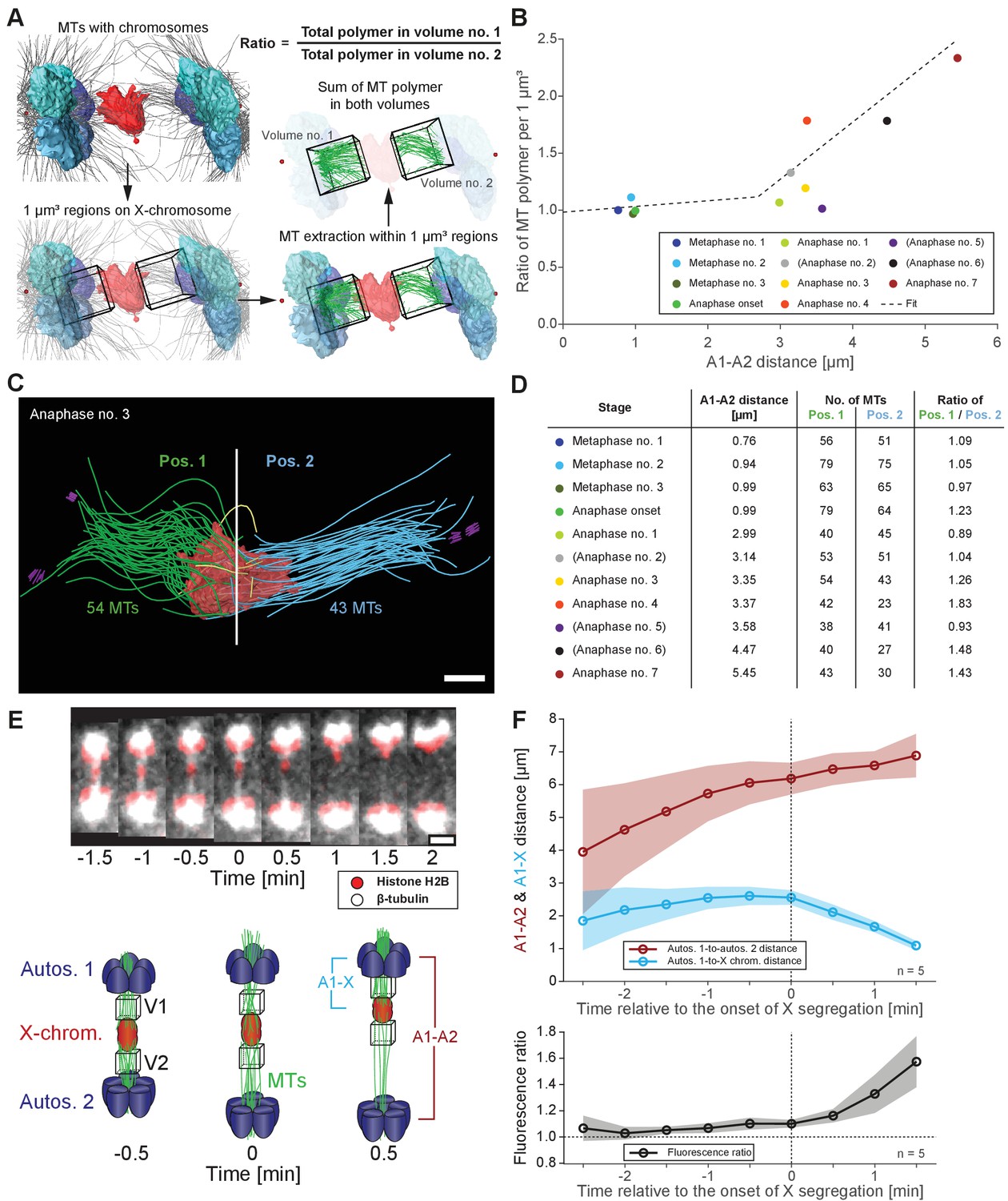
Resolution of the X chromosome to one side correlates with an asymmetry of microtubules.
(A) Left: three-dimensional model of an anaphase I spindle and definition of two equal volumes on opposite sides of the X chromosome. Right: Measurement of total polymer length within selected volumes of 1 µm3. (B) Graph showing the ratio of both volumetric measurements plotted against the autosome-to-autosome distance for the meiotic stages as shown in Figures 3 and 4 and Appendix 1—figure 4. A trend line was fitted to illustrate the increase in the asymmetry. (C) Deconstructed 3D model (data set anaphase no. 3) illustrating the microtubules associated with each side of the X chromosome (red), named pos. 1 (green) and pos. 2 (blue). Centrioles are shown in purple, microtubules not connected to the spindle poles in yellow. Scale bar, 500 nm. (D) Table showing the autosome 1-to-autosome 2 distance (A1, A2), the total number of microtubules for both positions and the calculated ratio for each data set (see Figures 3 and 4 and Appendix 1—figure 4 (data sets shown in parentheses)). (E) Upper panel: Maximum intensity projection images from live imaging showing microtubules labeled with β-tubulin::GFP (white) and chromosomes with histone H2B::mCherry (red). Time is given relative to the onset of X chromosome segregation (t = 0). Scale bar, 2 µm. Lower panel: Illustration of the measurement of fluorescence intensity in two volumes (V1, V2) of 1 µm3 at opposite sides of the X chromosome (red). Autosomes are in blue, microtubules in green. (F) Ratio of fluorescence intensities as measured in (E). Upper panel: autosomes 1-to-autosomes two distance (A1-A2, red) and autosomes 1-to-X chromosome distance (A1-X, blue) over time. Solid lines show the mean, shaded areas indicate the standard deviation. The onset of X chromosome movement is given as time point zero (t = 0). Lower panel: ratio of fluorescence intensities (V1/V2) for corresponding time points (black, time is relative to the onset of segregation of the X chromosome, t = 0; n = 5).
-
Figure 6—source data 1
Autosome-to-autosome distances and volumetric measurements for the meiotic stages shown in Figures 3 and 4 and Appendix 1—figure 4 used to generate Figure 6B.
- https://cdn.elifesciences.org/articles/50988/elife-50988-fig6-data1-v4.xlsx
Figure 7 with 2 supplements
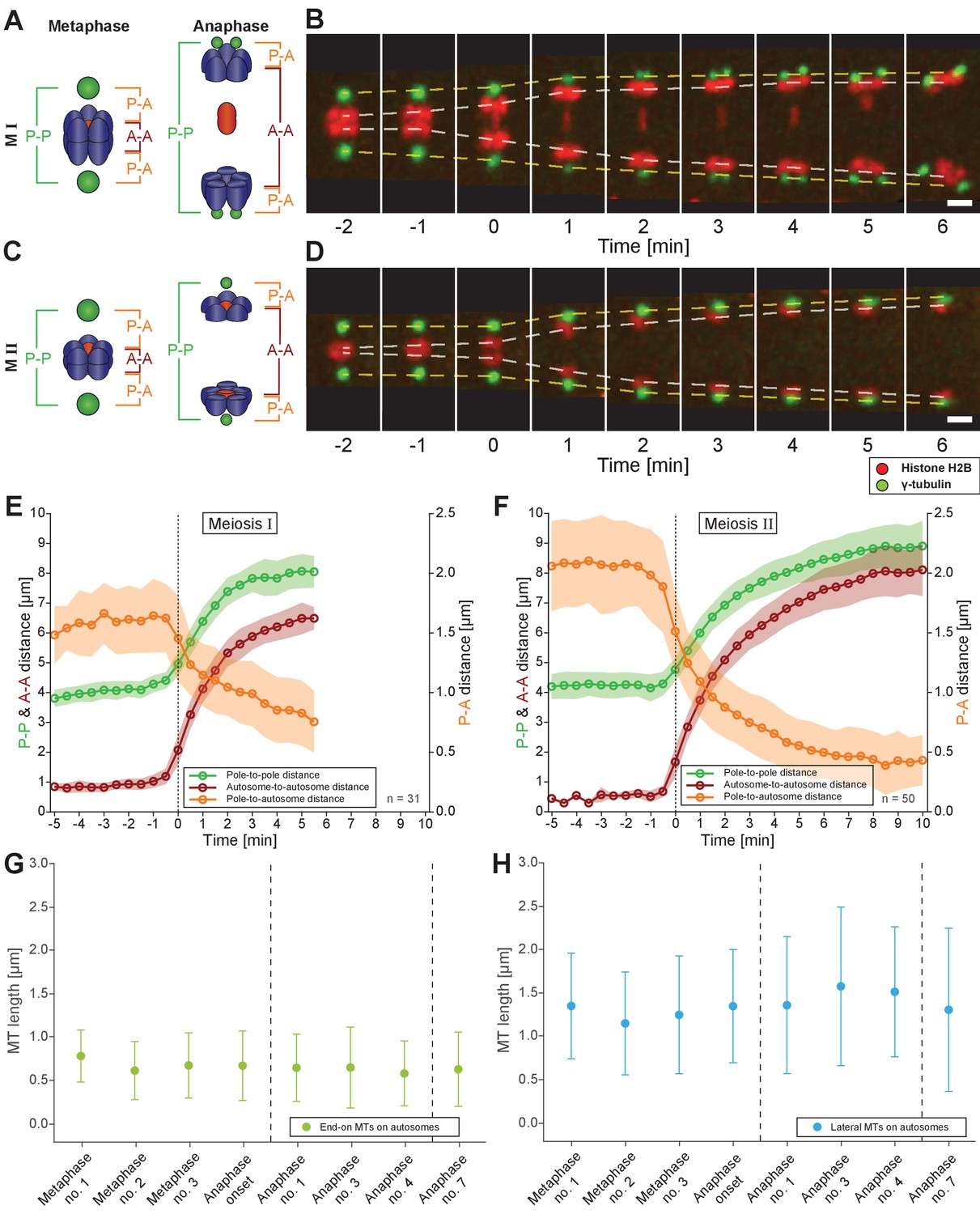
Spermatocyte meiotic spindles display both anaphase A and B movement.
(A) Schematic representation of metaphase and anaphase during meiosis I. Centrosomes are in green, autosomes in blue, and the univalent X chromosome in red. The pole-to-pole (P-P, green), autosome-to-autosome (A-A, red), and both pole-to-autosome distances (P-A, orange) are indicated. (B) Time series of confocal image projections of a spindle in meiosis I with centrosomes labeled with γ-tubulin::GFP (green) and chromosomes with histone H2B::mCherry (red). The separation of the centrosomes (yellow dashed line) and the autosomes (white dashed line) over time is indicated. Anaphase onset is time point zero (t = 0). Scale bar, 2 µm. (C) Schematic representation of metaphase and anaphase during meiosis II. (D) Separation of centrosomes and autosomes in meiosis II as in (F). Scale bar, 2 µm. (E) Quantitative analysis of autosome and centrosome dynamics in meiosis I show a decrease in pole-autosome distance that is characteristic of anaphase A. Anaphase onset is time point zero (t = 0). The mean and standard deviation is given (circles and shaded areas). (F) Quantitative analysis of autosome and centrosome dynamics in meiosis II. (G) Length distribution of end-on autosome-associated kinetochore microtubules at different stages of meiosis I. Dots show the mean, error bars indicate the standard deviation. Dashed lines indicate a grouping of the spindles according to the meiotic stages: metaphase/anaphase onset, mid anaphase and late anaphase (see also Appendix 1—figure 2). (H) Length distribution of laterally autosome-associated kinetochore microtubules at different stages of meiosis I.
-
Figure 7—source data 1
Measurements of autosome and centrosome dynamics from replicates used in Figure 7 .
- https://cdn.elifesciences.org/articles/50988/elife-50988-fig7-data1-v4.xlsx
Figure 7—video 1
Spindle dynamics in wild-type spermatocytes in meiosis I.
This video shows the first meiotic division in spermatocytes in living males. The strain was labeled with γ-tubulin::GFP (green) and histone H2B::mCherry (red) to visualize centrosomes and chromosomes, respectively. The image data were resampled to correct for the movements of the male worm during imaging. Time is given relative to the onset of anaphase I. Scale bar, 2 µm. This video corresponds to Figure 7D.
Figure 7—video 2
Spindle dynamics in wild-type spermatocyte meiosis II.
This video shows the second meiotic division in spermatocytes in living males. The strain was labeled with γ-tubulin::GFP (green) and histone H2B::mCherry (red) to visualize centrosomes and chromosomes, respectively. The image data were resampled to correct for the movements of the male worm. Time is given relative to the onset of anaphase II. Scale bar, 2 µm. This video corresponds to Figure 7F.
Figure 8
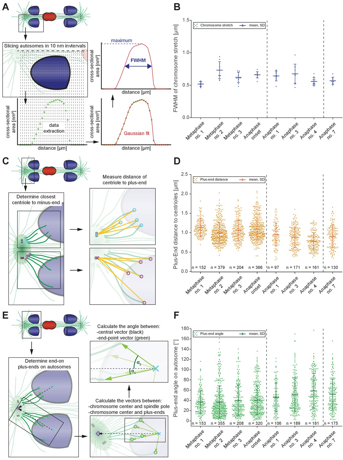
Changes in spindle geometry during anaphase A.
(A) Analysis of autosome stretching in anaphase I. Schematic representation showing how the full width half maximum (FWHM) of stretching along the pole-to-pole axis for a single autosome is assessed (see also Materials and methods). (B) FWHM of chromosome stretch for all autosomes at each meiotic stage shown in Figures 3 and 4. The mean, the standard deviation and the number of measurements (n = 10) for each meiotic stage are given. Dashed lines indicate a grouping of the spindles according to the meiotic stages: metaphase/anaphase onset, mid anaphase and late anaphase (see also Appendix 1—figure 2). Additional ANOVA results are shown in Appendix 1—figure 5G. (C) Schematic depicting the determination of the distance of individual kinetochore microtubule plus ends to the closest centriole. For each kinetochore microtubule (green line), the direct distance (yellow line) from the putative plus end to the respective centriole was measured (plus ends of kinetochore microtubules are shown in circles). (D) Distance of kinetochore microtubule plus-ends to centrioles for each meiotic stage. Additional ANOVA results are shown in Appendix 1—figure 5H. (E) Analysis of the attachment angle of end-on-associated autosomal kinetochore microtubules. The schematic illustrates the defined main axis for the measurements (dashed line from the center of each autosome to the center of the centrosome). The angle (α) between each line connecting the kinetochore microtubule plus-end and the autosome center (green lines) and the main axis (dashed line) was measured for each kinetochore microtubule. (F) Plot showing the angle measurements for all data sets. Additional ANOVA results are given in Appendix 1—figure 5I.
-
Figure 8—source data 1
Measurements for Full Width at Half-Maximum(FWHM) of replicates in each stage shown in Figures 3 and 4 used in Figure 8.
- https://cdn.elifesciences.org/articles/50988/elife-50988-fig8-data1-v4.xlsx
Appendix 1—figure 1
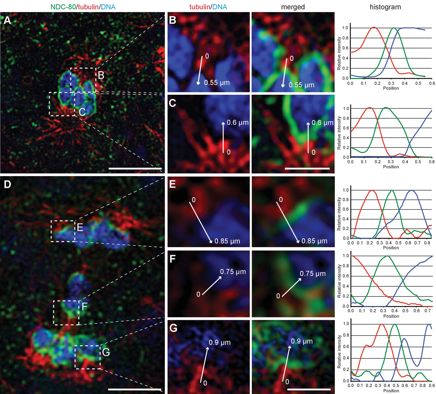
The outer kinetochore protein NDC80 localizes between chromosomes and microtubules at spermatocyte metaphase and anaphase I.
(A) Super-resolution fluorescence microscopy of metaphase I in fixed him-8(e1489) X0 males stained with antibodies against α-tubulin (red) and NDC-80 (green). DAPI stained DNA is in blue. Scale bar, 2 µm. (B–C) Enlargement of boxed regions as shown in (A) highlighting microtubule and NDC-80 localization relative to metaphase chromosomes. Normalized intensity values along the arrows for each staining pattern are plotted in the histograms (right panels). Scale bars, 0.5 µm. (D) Super-resolution fluorescence microscopy of anaphase I in him-8 X0 males. Imaging conditions were as given in (A). Scale bar, 2 µm. (E–G) Enlargement of boxed regions as shown in (A) highlighting microtubule and NDC-80 localization relative to separating chromosomes. Scale bar, 0.5 µm.
Appendix 1—figure 2

Comparison of electron tomographic and light microscopic data.
(A) Pole-to-pole distance plotted against the autosome-to-autosome distance for each tomographic data set (color coding is as shown in Figure 6B). Light microscopic measurements (Figure 7E) are shown in black. For the purpose of staging, the plot illustrates where the tomographic data sets are ‘positioned’ with respect to the averaged data from light microscopy (fitted dashed line in black) obtained. (B) Pole-to-autosome distance plotted against the autosome-to-autosome distance.
-
Appendix 1—figure 2—source data 1
Measurements of autosome-to-autosome and pole-to-autosome distances from replicates used in Appendix 1—figure 2.
- https://cdn.elifesciences.org/articles/50988/elife-50988-app1-fig2-data1-v4.xlsx
Appendix 1—figure 3
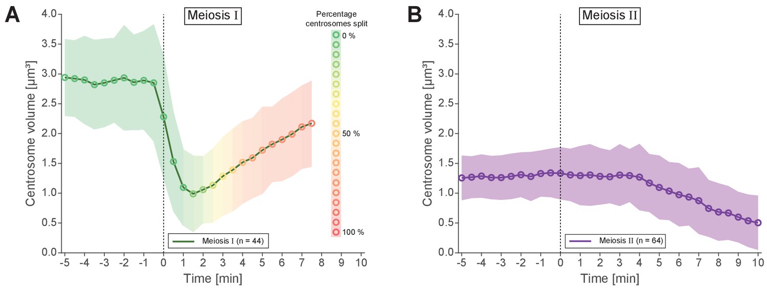
Analysis of centrosomal volumes in meiosis I and II.
(A) Plot showing centrosome volume in meiosis I over time. The 3D volume was measured in worms expressing γ-tubulin::GFP and histone H2B::mCherry. For each dataset a fixed threshold was defined to segment the outer border of the centrosome. The mean volume is plotted as a green line for unsplitted centrosomes and shown as an orange to red line for splitted centrosomes. The percentage of splitted centrosomes is indicated by this color change. For splitted centrosomes, the sum of both separated centrosomes was determined (n = 44). The standard deviation is depicted as a shaded area. (B) Centrosome volume over time (purple line) in meiosis II (n = 64).
-
Appendix 1—figure 3—source data 1
Measurements of centrosome volume from replicates used in Appendix 1—figure 3.
- https://cdn.elifesciences.org/articles/50988/elife-50988-app1-fig3-data1-v4.xlsx
Appendix 1—figure 4
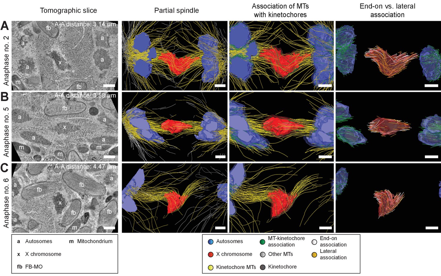
Visualization of partially reconstructed spindles in mid/late anaphase I.
(A) Mid anaphase spindle with a pole-to-pole distance of 3.14 µm. (B) Mid anaphase spindle with a pole-to-pole distance of 3.58 µm. (C) Mid anaphase spindle with a pole-to-pole distance of 4.47 µm. Left panels: tomographic slice showing the autosomes (a), and the univalent X chromosome (x) aligned along the spindle axis. Mitochondria (m) and fibrous body-membranous organelles (fb) are also indicated. Mid left panels: corresponding three-dimensional model illustrating the organization of the partially reconstructed spindle. Autosomes are in blue, the X chromosome in red, microtubules within a distance of 150 nm or closer to the chromosome surfaces in yellow and all other microtubules in gray. Mid right panels: association of microtubules with the kinetochores. Kinetochores are shown as semi-transparent regions around each chromosome. The part of each microtubule entering the kinetochore region around the holocentric chromosomes is in green. Right panels: visualization of end-on (white) versus laterally (orange) X chromosome-associated microtubules. The part of each microtubule entering the kinetochore region around the holocentric chromosomes is shown in green. The autosome-to-autosome distance (A-A) for each reconstruction is indicated in the left column. Scale bars, 500 nm.
Appendix 1—figure 5

Comparison of microtubule length distributions and spindle geometry (ANOVA).
(A) Length of end-on X chromosome-associated kinetochore microtubule for each tomographic data set as shown in Figure 5A. The mean, the standard deviation and single measurements for each meiotic stage are given. Results of a one-way analysis of variance (ANOVA) of all data sets against each other are shown. Level of significance: * is p<=0.05; ** is p<=0.01; and *** is p<=0.001. (B) Length of lateral X chromosome-associated kinetochore microtubules corresponding to Figure 5B. (C) Tortuosity of end-on X chromosome-associated kinetochore microtubules corresponding to Appendix 1—figure 6B. (D) Tortuosity of lateral X chromosome-associated kinetochore microtubules corresponding to Appendix 1—figure 6B. (E) Length of end-on autosome-associated kinetochore microtubules corresponding to Figure 7G. (F) Length of lateral autosome-associated kinetochore microtubules corresponding to Figure 7H. (G) FWHM of the chromosome stretch for each meiotic stage corresponding to Figure 8B. (H) Distance of autosomal kinetochore microtubule plus-ends to closest centriole for each meiotic stage corresponding to Figure 8D. (I) Measurement of attachment angles of autosomal end-on associated kinetochore microtubules as given in Figure 8F.
Appendix 1—figure 6

Tortuosity of X chromosome-associated microtubules during anaphase I.
(A) Schematic drawing illustrating the shape of X chromosome-associated kinetochore microtubules. Both end-on (yellow) and laterally associated microtubules (purple) are shown (left panels). The tortuosity of each microtubule is given by the spline length (red dotted lines; right panel) divided by the end-to-end length (black dotted lines). Dashed lines indicate a grouping of the spindles according to the meiotic stages: metaphase/anaphase onset, mid anaphase and late anaphase (see also Appendix 1—figure 2). (B) Plots showing the tortuosity of end-on (top) and laterally (bottom) associated kinetochore microtubules. The meiotic stages correspond to the data sets as shown in Figures 3 and 4. Mean, standard deviation and individual measurements are given for each data set.
-
Appendix 1—figure 6—source data 1
Measurements of tortuosity of end-on and lateral microtubules from replicates used in Appendix 1—figure 6.
- https://cdn.elifesciences.org/articles/50988/elife-50988-app1-fig6-data1-v4.xlsx
Appendix 1—figure 7 with 1 supplement

Organization and dynamics of tra-2(e1094) spindles in meiosis I.
(A) Time series of confocal image projections of three examples of tra-2(e1094) mutant spindles in meiosis I. Microtubules (β-tubulin::GFP) and chromosomes (histone H2B::mCherry) are visualized in green and red, respectively. Anaphase onset is time point zero (t = 0). Chromosome segregation is also visualized in kymographs (right panels). The start of the separation of the autosomes is indicated by a dashed line (orange). Scale bars (white), 2 µm; time bar (blue), 2 min. (B) Quantitative analysis of spindle elongation (pole-to-pole distance) over time in meiosis I in wild-type (green) and tra-2(e1094) (blue) spindles. Anaphase onset is time point zero (t = 0). The mean and standard deviation is given (circles and shaded areas). (C) Tomographic slice through a partial tra-2(e1094) mutant spindle in anaphase I (left panel). Autosomes (a), mitochondria (m) and FB-MOs (fb) are indicated. Three-dimensional model of the same tra-2(e1094) mutant spindle (right panel). Chromosomes are in blue, microtubules within a distance of 150 nm or closer to the chromosome surfaces in yellow and all other microtubules in white. The spindle midzone is indicated (red rectangle). Scale bars, 500 nm.
-
Appendix 1—figure 7—source data 1
Measurements of pole-to-pole distance over time in replicates used in Appendix 1—figure 7B.
- https://cdn.elifesciences.org/articles/50988/elife-50988-app1-fig7-data1-v4.xlsx
Appendix 1—figure 7—video 1
Organization of tra-2 spindles in meiosis I.
This video shows a three-dimensional model of a tra-2(e1094) mutant spindle at anaphase I. Chromosomes are shows in blue, kinetochore microtubules in yellow, other microtubules in white. This video corresponds to Appendix 1—figure 7C.
Appendix 1—figure 8

Composition of the spindle midzone in male meiosis I.
(A) Confocal light microscopy of the spindle midzone in him-8(e1489) and tra-2(e1094) spermatocytes. For comparison, the spindle midzone in wild-type oocytes in anaphase I is also shown. Samples were stained with antibodies against three different proteins: AuroraBAIR-2, CLASPCLS-2 and MKLP1ZEN-4. Stained proteins are shown in green, chromosomes in red. Scale bar, 2 µm. (B) Time series of confocal image projections of wild-type meiosis I in males (upper row) and hermaphrodite spermatocytes (lower row). The microtubule bundling protein PRC1SPD-1 (SPD-1::GFP, white) and the chromosomes (histone H2B::mCherry, red) are visualized. Anaphase onset is time point zero (t = 0). White arrowheads mark the position of the unpaired X chromosome in meiosis I. Chromosome segregation is also visualized in kymographs (right panels; the start of the separation of the autosomes is indicated by a dashed orange line). Scale bars (white), 2 µm; time bar (blue), 2 min.
Appendix 1—figure 9
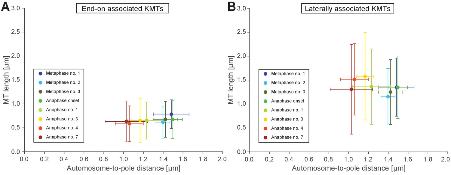
Length of end-on and laterally autosome-associated microtubules.
-
Appendix 1—figure 9—source data 1
Measurements of pole-to-autosome and microtubule length in each stage shown in Figures 3 and 4 used in Appendix1-figure 9-source data1.
- https://cdn.elifesciences.org/articles/50988/elife-50988-app1-fig9-data1-v4.xlsx
Appendix 1—figure 10
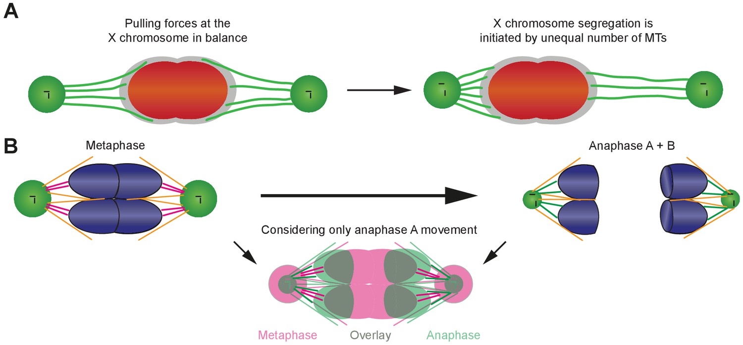
Proposed models of chromosome movements in meiosis I.
(A) Proposed tug-of-war model for the initiation of X chromosome segregation in anaphase I in males. The X chromosome is shown in red, the holocentric kinetochore in gray, and the X chromosome-associated kinetochore microtubules in green. Left panel: At metaphase I, pulling forces at the X chromosome are in balance. Right panel: segregation of the X chromosome is initiated by an imbalance of forces, obvious by an unequal number of kinetochore microtubules associated with the opposite sides of the X chromosome. In anaphase I, the X is proposed to move to the side with more attached kinetochore microtubules. (B) Model illustrating the changes in spindle geometry. Left upper panel is metaphase; right upper panel is anaphase; lower panel shows combining anaphase A and B. Chromosomes are shown in blue, centrosomes in green, centrioles in black. Laterally associated microtubules are illustrated in orange. The end-on associated kinetochore microtubules (magenta in metaphase and green in anaphase) have the same length at both stages. The lower panel is an overlay of metaphase (magenta) with anaphase A (green, anaphase B movement was not considered) to show the relative movement of the autosomes with respect to the centrosomes. A simultaneous rounding of the autosomes, a shrinking of the volume of the centrosomes and a change in the attachment angle of the microtubules is illustrated.
Videos
Video 1
Visualization of end-on or laterally associated kinetochore microtubules.
This video illustrates the classification of kinetochore microtubules according to their type of association to chromosomes. Chromosomes are shown in light teal, the holocentric kinetochore area surrounding the chromosomes in dark semi-transparent teal. End-on associated kinetochore microtubules are shown in white, laterally associated microtubules in orange).
Tables
Table 1
Analysis of tomographic data sets used throughout this study.
| Full data sets | Partial data sets | ||||||||||
|---|---|---|---|---|---|---|---|---|---|---|---|
| Spindle parameters | Metaphase no. 1 | Metaphase no. 2 | Metaphase no. 3 | Anaphase onset | Anaphase no. 1 | Anaphase no. 3 | Anaphase no. 4 | Anaphase no. 7 | Anaphase no. 2 | Anaphase no. 5 | Anaphase no. 6 |
| MTs total | 1729 | 2406 | 1689 | 2051 | 1405 | 1540 | 1403 | 1881 | (893) | (671) | (246) |
| MTs within 150 nm from chromosomes (KMTs) | 524 | 912 | 650 | 794 | 633 | 821 | 752 | 944 | (580) | (499) | (160) |
| End-on associated KMTs on X-chromosome | 29 | 38 | 38 | 53 | 27 | 50 | 38 | 42 | 57 | 30 | 43 |
| Lateral associated KMTs on X-chromosome | 79 | 34 | 91 | 22 | 61 | 55 | 33 | 34 | 47 | 52 | 28 |
| End-on associated KMTs on autosomes | 154 | 355 | 199 | 318 | 106 | 189 | 181 | 175 | |||
| Lateral associated KMTs on autosomes | 262 | 485 | 321 | 400 | 437 | 527 | 500 | 692 | |||
| Autosome-to-autosome distance [µm] | 0.76 | 0.94 | 0.99 | 1.00 | 2.98 | 3.35 | 3.37 | 5.44 | (3.14) | (3.58) | (4.47) |
| Autosomes1-to-X distance [µm] | 0.37 | 0.43 | 0.43 | 0.47 | 1.45 | 1.45 | 1.37 | 1.95 | (1.54) | (1.71) | |
| Autosomes2-to-X distance [µm] | 0.39 | 0.51 | 0.56 | 0.54 | 1.56 | 2.02 | 1.99 | 3.51 | (1.72) | (1.90) | |
| Pole-to-pole distance [µm] | 3.10 | 3.41 | 3.45 | 3.51 | 4.97 | 5.22 | 4.99 | 7.04 | |||
| Pole1-to-X distance [µm] | 1.64 | 1.66 | 1.66 | 1.62 | 2.60 | 2.29 | 2.21 | 2.69 | |||
| Pole2-to-X distance [µm] | 1.48 | 1.76 | 1.80 | 1.90 | 2.39 | 3.04 | 2.77 | 4.38 | |||
| Autosome-to-centrosome distance [µm] | 1.18 | 1.24 | 1.23 | 1.26 | 1.00 | 0.94 | 0.82 | 0.83 | |||
| Mother-to-daughter centriole distance [µm] | 0.26 | 0.21 | 0.27 | 0.35 | 0.37 | 0.73 | 0.74 | 1.11 | |||
| Original name of data set | T0391_worm13 metaphase01 | T0391_worm14 metaphase | T0391_worm13 metaphase02 | T0391_worm13 meta-anaphase01 | T0391_worm05 anaphase02 | T0391_worm08 lateanaphase | T0391_anaphase01 early | T0391_worm09 late_anaphase | T0391_worm07b | T0391_worm06 | T0391_worm02 |
| Number of sections | 14 | 11 | 14 | 25 | 14 | 17 | 11 | 30 | 8 | 4 | 6 |
| Est. tomographic volume [µm³] | 102.33 | 94.70 | 107.52 | 115.12 | 113.96 | 131.92 | 101.51 | 268.31 | 36.99 | 18.52 | 30.37 |
-
The table summarizes all microtubule numbers and distances as measured within the electron tomographic reconstructions in this study. A kinetochore microtubule (KMT) is defined as a microtubule that is at least 150 nm from the surface of a chromosome. KMTs are sub-divided into end-on and lateral associated MTs. End-on KMTs are defined as pointing towards the chromosome surface, lateral MTs are all remaining KMTs. Distances were measured between the geometric centers of autosomes (mean position of individual autosomes), centrosomes (center point of both centrioles) and centrioles (between the centers of the mother and daughter centriole). Tomographic volumes were estimated by multiplying the X-Y dimensions of each tomogram with the number of sections (with a section thickness of 300 nm).
Table 2
Measurements of spindle dynamics in male meiosis.
| Distance | Spindle parameter | Meiosis I | Meiosis II | ||
|---|---|---|---|---|---|
| Mean | SD | Mean | SD | ||
| P-P1 | Initial spindle length (metaphase) | 4.1 µm | ±0.3 µm | 4.2 µm | ±0.4 µm |
| Final spindle length (end of anaphase) | 8.0 µm | ±0.6 µm | 8.8 µm | ±0.8 µm | |
| Initial rate (1 st minute) | 1.29 μm/min | ±0.36 μm/min | 1.11 μm/min | ±0.42 μm/min | |
| Duration of elongation | 3–4 min | 8–9 min | |||
| A-A2 | Initial spindle length (metaphase) | 0.9 µm | ±0.2 µm | 0.6 µm | ±0.2 µm |
| Final spindle length (end of anaphase) | 6.5 µm | ±0.4 µm | 8.0 µm | ±0.8 µm | |
| Initial rate (1 st minute) | 2.07 µm/min | ±0.37 μm/min | 2.16 µm/min | ±0.32 μm/min | |
| Duration of elongation | 4–5 min | 8–9 min | |||
| P-A3 | Initial spindle length (metaphase) | 1.6 µm | ±0.3 µm | 2.0 µm | ±0.4 µm |
| Final spindle length (end of anaphase) | 0.8 µm | ±0.3 µm | 0.4 µm | ±0.2 µm | |
| Initial rate (1 st minute) | −0.39 µm/min | ±0.27 μm/min | −0.64 µm/min | ±0.33 μm/min | |
-
Distances: 1P-P, pole-to-pole distance; 2A-A, autosome-to-autosome distance; 3P-A, pole-to-autosome distance. Initial spindle length is given at metaphase, final distance refers to the end of anaphase when spindle elongation plateaus. Values are given as mean values (± standard deviation, SD). The numbers of analyzed spindles are: n = 31 for meiosis I; n = 50 for meiosis II.
Key resources table
| Reagent type (species) or resource | Designation | Source or reference | Identifiers | Additional information |
|---|---|---|---|---|
| Genetic reagent C. elegans | N2 | (Brenner, 1974) | ||
| Genetic reagent C. elegans | ANA0072 | (Nahaboo et al., 2015) | ||
| Genetic reagent C. elegans | CB1489 | (Herman and Kari, 1989; Phillips et al., 2005) | ||
| Genetic reagent C. elegans | CB2580 | (Hodgkin, 1985) | ||
| Genetic reagent C. elegans | MAS91 | (Han et al., 2015) | ||
| Genetic reagent C. elegans | MAS96 | M. Srayko, Alberta | Strain maintained in the Srayko lab | |
| Genetic reagent C. elegans | TMR17 | this study | Strain maintained in the Müller-Reichert lab | |
| Genetic reagent C. elegans | TMR18 | this study | Strain maintained in the Müller-Reichert lab | |
| Genetic reagent C. elegans | TMR26 | this study | Strain maintained in the Müller-Reichert lab | |
| Genetic reagent C. elegans | XC110 | this study | Strain maintained in the Chu lab | |
| Genetic reagent C. elegans | XC116 | this study | Strain maintained in the Chu lab | |
| Genetic reagentC. elegans | SP346 | (Madl and Herman, 1979) | ||
| Genetic reagent E. coli | OP50 | (Brenner, 1974) | ||
| Antibody | Rabbit polyclonal anti-NDC-80 | Novus Biologicals | Novus Biologicals: 42000002; RRID:AB_10708818 | 1:200 |
| Antibody | Mouse monoclonal anti-α-tubulin | Sigma-Aldrich | Sigma-Aldrich: T6199; RRID:AB_477583 | 1:200 |
| Antibody | Mouse monoclonal anti-a-tubulin + FITC | Sigma-Aldrich | Sigma-Aldrich: F2168; RRID:AB_476967 | 1:50 |
| Antibody | Goat polyclonal anti-rabbit + AlexaFluor 488 | Invitrogen | Invitrogen: A11034; RRID:AB_2576217 | 1:200 |
| Antibody | Goat polyclonal anti-mouse + AlexaFluor 488 | Invitrogen | Invitrogen: A11001; RRID:AB_2534069 | 1:200 |
| Antibody | Goat polyclonal anti-mouse + AlexaFluor 564 | Invitrogen | Invitrogen: A11010; RRID:AB_2534077 | 1:200 |
| Antibody | Donkey polyclonal anti-rabbit + Cy3 | Jackson ImmunoResearch | Jackson ImmunoResearch: 711-165-152; RRID:AB_2307443 | 1:500 |
| Antibody | Rabbit polyclonal anti-KNL-1 | (Desai et al., 2003) | 1:500 | |
| Antibody | Rabbit polyclonal anti-KNL-3 | (Cheeseman et al., 2004) | 1:500 | |
| Antibody | Rabbit polyclonal anti-AIR-2 | (Schumacher et al., 1998) | 1:200 | |
| Antibody | Rabbit polyclonal anti-CLS-2 | (Espiritu et al., 2012) | 1:200 | |
| Antibody | Rabbit polyclonal anti-ZEN-4 | (Powers et al., 1998) | 1:200 | |
| Chemical compound, drug | Polystyrene microbeads solution (0.1 µm) | Polysciences | Polysciences:00876–15 | |
| Chemical compound, drug | Hexadecene | Merck | Merck: 822064 | |
| Chemical compound, drug | BSA (fraction V) | Carl Roth | Carl Roth: 8076.2 | |
| Chemical compound, drug | Osmium tetroxide | EMS | EMS: 19100 | |
| Chemical compound, drug | Uranyl acetate | Polysciences | Polysciences: 21447–25 | |
| Chemical compound, drug | Epon/Araldite epoxy resin | EMS | EMS: 13940 | |
| Chemical compound, drug | Colloidal gold (15 nm) | BBI | BBI: EM.GC15 | |
| Other | Type-A aluminum planchette | Wohlwend | Wohlwend: 241 | |
| Other | Type-B aluminum planchette | Wohlwend | Wohlwend: 242 | |
| Software, algorithm | Code for Kymograph creation | this study | Python code provided as supplemental information | |
| Software, algorithm | Code for Image volume resampling | this study | Python code provided as supplemental information | |
| Software, algorithm | arivis Vision4D | Arivis AG (https://www.arivis.com/en/imaging-science/arivis-vision4d) | Versions 2.9–2.12 | |
| Software, algorithm | IMOD | (Kremer et al., 1996) (https://bio3d.colorado.edu/imod/) | Version 4.8.22 | |
| Software, algorithm | ZIBAmira | (Stalling et al., 2005) (https://amira.zib.de/) | Versions 2016.47–2017.55 |
Additional files
-
Source code 1
Kymograph.
This script needs two 3D coordinates and 3D image data as an input and creates a 2D line scan in between the two input coordinates according to the settings in the script. If a time series is used this algorithm creates a kymograph.
- https://cdn.elifesciences.org/articles/50988/elife-50988-code1-v4.py
-
Source code 2
Volume resampling.
This script needs two 3D coordinates and 3D image data as an input and creates a spatially reoriented and resampled 3D data set in between the two input coordinates according to the settings in the script. The center line (spindle axis) in between the two input coordinates is positioned in the z-dimension of the output data set. If a time series is used this algorithm creates a resampled 3D data set over time.
- https://cdn.elifesciences.org/articles/50988/elife-50988-code2-v4.py
-
Transparent reporting form
- https://cdn.elifesciences.org/articles/50988/elife-50988-transrepform-v4.pdf
-
Appendix 1—figure 2—source data 1
Measurements of autosome-to-autosome and pole-to-autosome distances from replicates used in Appendix 1—figure 2.
- https://cdn.elifesciences.org/articles/50988/elife-50988-app1-fig2-data1-v4.xlsx
-
Appendix 1—figure 3—source data 1
Measurements of centrosome volume from replicates used in Appendix 1—figure 3.
- https://cdn.elifesciences.org/articles/50988/elife-50988-app1-fig3-data1-v4.xlsx
-
Appendix 1—figure 6—source data 1
Measurements of tortuosity of end-on and lateral microtubules from replicates used in Appendix 1—figure 6.
- https://cdn.elifesciences.org/articles/50988/elife-50988-app1-fig6-data1-v4.xlsx
-
Appendix 1—figure 7—source data 1
Measurements of pole-to-pole distance over time in replicates used in Appendix 1—figure 7B.
- https://cdn.elifesciences.org/articles/50988/elife-50988-app1-fig7-data1-v4.xlsx
-
Appendix 1—figure 9—source data 1
Measurements of pole-to-autosome and microtubule length in each stage shown in Figures 3 and 4 used in Appendix1-figure 9-source data1.
- https://cdn.elifesciences.org/articles/50988/elife-50988-app1-fig9-data1-v4.xlsx
Download links
A two-part list of links to download the article, or parts of the article, in various formats.
Downloads (link to download the article as PDF)
Open citations (links to open the citations from this article in various online reference manager services)
Cite this article (links to download the citations from this article in formats compatible with various reference manager tools)
Male meiotic spindle features that efficiently segregate paired and lagging chromosomes
eLife 9:e50988.
https://doi.org/10.7554/eLife.50988


